Spatial calibration of large volume photogrammetry based metrology systems

1

Spatial calibration of large volume photogrammetry based

metrology systems

R Summan1_{, S G Pierce}1_{, C N Macleod}1_{, G Dobie}1_{, T Gears}2 _{and W Lester}3_{, P}

Pritchett3_{, P Smyth}3

1 _{Centre for Ultrasonic Engineering, University of Strathclyde, 204 George Street,}

Glasgow UK, G1 1XW ([email protected])

2 _{Hexagon Metrology Ltd, Metrology House, Halesfield 13, Telford UK, TF74PL} 3 _{Vicon Motion Systems Ltd. Oxford, 14 Minns Business Park West Way, Oxford,}

OX2 0JB

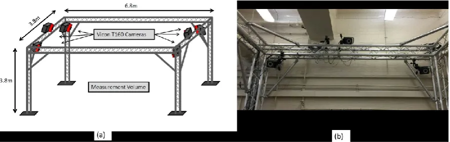
Abstract. Photogrammetry systems are used extensively as volumetric measurement tools in a diverse range of applications including gait analysis, robotics and computer generated animation. For precision applications the spatial inaccuracies of these systems are of interest. In this paper, an experimental characterisation of a six camera Vicon T160 photogrammetry system using a high accuracy laser tracker is presented. The study was motivated by empirical observations of the accuracy of the photogrammetry system varying as a function of location within a measurement volume of approximately 100m3_{. Error quantification was implemented}

through simultaneously tracking a target scanned through a sub-volume (27m3_{) using both}

systems. The position of the target was measured at each point of a grid in four planes at different heights. In addition, the effect of the use of passive and active calibration artefacts upon system accuracy was investigated. A convex surface was obtained when considering error as a function of position for a fixed height setting confirming the empirical observations when using either calibration artefact. Average errors of 1.48 mm and 3.95 mm were obtained for the active and passive calibration artefacts respectively. However, it was found that through estimating and applying an unknown scale factor relating measurements, the overall accuracy could be improved with average errors reducing to 0.51 mm and 0.59 mm for the active and passive datasets respectively. The precision in the measurements was found to be less than 10 μm for each axis.

1. Introduction

A number of commercially available multi-camera real time photogrammetry systems [1, 2, 3], are used extensively in applications such as gait analysis [4], animation in the entertainment industry [5] and increasingly as tracking systems in robotics [6, 7, 8, 9]. The technique is attractive due to the associated benefits of fully non-contact sensing, six degree-of-freedom (6 DOF) measurement, high temporal sampling rates (up to kHz frequencies), multiple simultaneous object tracking (up to 1000’s) and the potential for high accuracy and precision measurements. The accuracy of such systems is dependent upon numerous variables such as the number and resolution of cameras deployed, the dimensions of the measurement volume, the positional configuration of cameras around the measurement volume and the accuracy of the intrinsic and extrinsic parameters computed from the calibration procedure for each camera.

2 400 x 300 x 300 mm3 volume. Under optimal conditions the absolute error and precision for displacements of 20 µm were 1.2 - 1.8 µm and 1.5 - 2.5 µm. In [12], the authors consider the suitability of a two camera Qualisys ProReflex-MCU120 (658 x 500 pixels, CCD) for measuring micro displacements of teeth. In a field of view of size 68.18 x 51.14 mm, the accuracy of displacements ranging from 20 - 200µm, was found to be ±1.17%, ±1.67% and ± 1.31% in axis wise terms. The corresponding standard deviations were ±1.7 µm, ±2.3 µm and ±1.9 µm. The authors in [13] present a systematic experiment to determine the static accuracy and precision of a Vicon 460 system composed of five Mcam-60 cameras (1012 x 987 pixels, CMOS). The experiment was conducted for a 180 x 180 x 150 mm3 _{volume suitable for the capture of small magnitude} biomechanical motion. Dense accuracy measurements were obtained by driving a retro-reflective target affixed to an XYZ scanner (15 µm linear encoder accuracy) to 294 positions according to a 7 x 7 x 6 grid with 30 mm uniform spacing. The influence of several variables was considered: camera positioning around the volume; manual versus scanner based dynamic calibration (controlled arbitrary path); error associated with measurements outside the calibrated volume through calibrating a 90 x 90 x 75 mm3 _{sub-volume; marker size and use of lens filtering. Following analysis of the effect of} different variable combinations, the optimal set of variables yielded an overall accuracy of 63 ± 5 µm and 15 µm precision. In general it is concluded that major factors in determining overall accuracy include the arrangement of cameras, the marker size (larger markers promoting greater accuracy) and lens filtering to smooth irregular target boundaries. The above studies were confined to small measurement volumes of no more than 0.04 m3_{, and errors outside the calibration volume were} significantly greater as would be expected. These small measurement volumes are at least 3 orders of magnitude smaller than the present authors’ interests where our application for photogrammetry tracking relates to automated robotic inspection [8, 14]. Our research into accurate spatially correlated non-destructive testing (NDT) measurements uses a combination of both mobile semi-autonomous robots [14] and fixed 6 axis industrial robots [15] to deliver NDT measurements to a variety of test samples. The typical measurement volume exceeds 100 m3 _{and our applications demand absolute} accuracies of significantly less than 1 mm (industrial robot repeatability can routinely attain values of 100s of µm or better over their full working envelope).

Accuracy investigations for larger volumes have typically considered only a small region of the measurement volume [16, 17]. In [16], the authors compare the accuracy of several motion capture systems in a gait analysis context. A subject holding a rigid bar with targets affixed 900 mm apart was instructed to traverse a 3 m linear path through the measurement volume (area 10 m x 6 m). Photogrammetry systems composed of between two and six cameras were used to estimate the length of the bar. In this study, the mean absolute errors varied substantially between 0.53 mm and 18.42 mm. In [18] a “principal points indirect estimate - PIE” approach is reported to provide a rapid calibration approach with an error of 0.37 mm RMS over a volume with a diagonal approximately 1.5 m in length. Accuracy studies for larger volumes, on the scale of 100’s m3_{, typical of robotics} applications have not been reported in the literature. This is surprising as many UAV tracking applications [6] are therefore making unwarranted assumptions about overall system accuracy performance.

There exist a number of commercially available photogrammetry systems for non-contact, high accuracy, measurement of large structures [19, 20] using retro-reflective/white light targets. These systems can provide sub-millimetre accuracy but operate offline. The use of photogrammetry systems in very large scale environments (on the scale of km) is the domain of target-less systems for obvious practicality reasons. Single and multiple camera based systems are used extensively in robotics applications for vehicle pose estimation and environment modelling [21]. Since the target geometry is not known a priori, such systems offer less accuracy than those using targets. Indeed, systems such as that presented in the paper are often used to verify the accuracy of algorithms used by target-less systems.

3 calibrated volume. The error associated with the positional estimates from this system were considered over a measurement volume of dimension 3.9 x 3.05 x 2.3 m3 (27 m3) A high accuracy and precision laser tracker Leica absolute tracker AT901B [22] was employed to provide ground truth measurements of the position of a target scanned in four planes dividing the measurement volume vertical height. With reference to the variables identified in [13], an optimal camera arrangement was adopted such that overlap amongst the camera field of views was maximised thus ensuring at least two cameras were available for triangulation at any point in the volume. Dense accuracy measurements were collected inside the calibrated region using large markers of diameter 38.1 mm. The variable of interest in this article centres upon the choice of calibration artefact used for dynamic calibration. The dynamic calibration procedure requires a calibration artefact with known dimensions to be swept through the volume enclosed by the cameras. From the resultant point cloud the relative pose and optical parameters for each camera are determined. These parameters can have significant impact upon system accuracy as they directly affect how a 3D world point is projected onto a 2D image point. Two datasets were collected using different calibration artefacts. The first employed standard retro-reflecting spheres to reflect IR light projected from the cameras, while the second employed actively modulated light emitting diodes (LEDs) to provide active illumination.

The contributions of this paper are threefold: firstly dense spatial measurements over a large volume representative of real robotics applications are reported. Secondly an investigation of the effect of calibration artefact on system accuracy is carried out. Thirdly, an unknown scale factor relating the data from the two systems is identified and subsequently estimated.

2. Experimental methodology for spatial calibration

This section of the paper outlines the experimental approach adopted to make simultaneous measurements between the Vicon motion tracking system and the Leica AT901B laser tracker (used to provide a high accuracy ground truth measurement). Simultaneous measurements were recorded from both systems whilst monitoring a common custom-designed target which was spatially sampled throughout the large measurement volume. A number of specific sub-tasks were identified as being critical to maintaining accuracy of the overall measurement and these are dealt with individually below.

2.1 Vicon motion capture system

4 Figure 1 – (a) Positioning of six camera T160 Vicon system around measurement volume (b) Image of real frame

2.2 Photogrammetry system camera calibration

Dynamic calibration [10] is a key step in setting up a precision photogrammetry measurement system. It determines the 3D position and orientation of each camera (the extrinsic parameters) as well as the internal optical and lens distortion parameters (the intrinsic parameters) associated with each camera. The parameters are estimated from the point cloud that results from sweeping a calibration artefact through the volume, with the objective of sampling every part of the volume that will be used during online operation. The error associated with these parameters manifests as a systematic error in the overall accuracy of the system. The importance of these parameters may be understood through the equation mapping a 3D world point, X, into a 2D image point on the camera imaging plane, x, for a single camera [23]:

[ (1)

where K is

f 0 p_x 0 f p

0 0 1

(2)

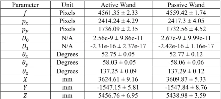
which represents the focal length, f , and the principal point (px , py). The 3D rotation, R, and translation vector, t, of the camera are contained in the matrix [R|t] while g is the function that removes lens distortion. The two different calibration artefacts used throughout the study are shown in Figure 2.

5 θy and θz. The results show that across ten trials the estimated position of the camera can vary considerably.

Figure 2 - Calibration artefacts, (a) Active calibration Wand (b) Passive calibration wand

Parameter Unit Active Wand Passive Wand

Pixels 4561.35 ± 2.33 4559.42 ± 1.74 Pixels 2414.24 ± 4.29 2417.3 ± 4.05

Pixels 1736.09 ± 2.35 1732.56 ± 4.52 N/A 2.56e-9 ± 9.86e-11 2.67e-9 ± 9.99e-11 N/A -2.31e-16 ± 2.37e-17 -2.42e-16 ± 1.16e-17 Degrees 52.75 ± 0.05 52.77 ± 0.12 Degrees -58.03 ± 0.05 -58.06 ± 0.06 Degrees 137.25 ± 0.09 137.29 ± 0.12 mm 3624.61 ± 9.16 3609.87 ± 5.33 mm -1547.15 ± 5.81 -1547.84 ± 8.76 mm 5456.76 ± 6.95 5438.98 ± 3.59

Table 1- Mean and standard deviation in parameters computed from calibration with the active and passive wands

2.3 Ground truth measurement system

6 Figure 3 - (a) AT Controller 900 running EmScon software (b) Leica Absolute Tracker AT901-B mounted on heavy

duty tripod (c) Tracking head that projects laser (d) Interferometer datum point

2.4 Target Object Design

A fundamental challenge in this study was to devise a test object that both measurement systems could track simultaneously as it was moved throughout the measurement volume. Both systems employed quite different approaches to position measurement; the Vicon system by estimating the centre of a retro-reflecting target from multiple images of the whole target, the Leica tracker through the tracking of a retro-reflective prism. This is in contrast to previous studies that have made use of targets of known lengths with rod-like geometry [16] or have compared relative motions which did not require alignment between the tracking systems [13].

A standard laser tracker target consists of a precision retro-reflector mounted inside a steel spherical shell (a precision machined ball bearing). Standard sizes for the spherical shell are 12.5 mm and 31.8 mm diameters corresponding to imperial sizes of 0.5 and 1.5 inch respectively. By mounting the retro-reflective prism in this fashion, it is possible to position the outer spherical shell into magnetic mounts with a high repeatability (assuming that the magnetic mount surfaces are carefully cleaned of surface debris). This repeatability was evaluated experimentally and it was found that the centre deviation of the reflector over ten trials had a mean value of 3.7 μm per axis. The key to the positioning consistency of the actual retro-reflective prism, lies in the centring accuracy of the prism inside the steel shell. For this study a reflector with the highest level of centring accuracy was selected (< ± 0.006 mm).

7 comparison to a wrapped tape version. However, it was found in practice that the resulting markers displayed a higher variation in brightness across the surface than the retroreflective tape based markers – this led to an unwanted potential bias in the centre estimate. In addition, the glass bead retroreflector targets did not reflect IR light as effectively as the tape based markers and there was significant variation in the reflected light across the volume. Given these shortcomings, tape based markers were used for the remainder of the study.

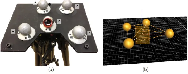
The test object used in the experiment consisted of five magnetic holders mounted upon an aluminium plate. The position of the prism reflector and thus Vicon target centres was initially measured using the AT901 laser tracker and retro-reflective prism target in each holder successively. The four outer targets (A, B, C, D) were used to define a Vicon virtual object (with 6 degree of freedom tracking), and a centre co-incident with the final target (E). In this fashion the (x, y, z) coordinate centre of the Vicon tracked object coincided (to within the tape thickness error) with the centre of the laser tracked retroreflective prism. This approach allowed the simultaneous acquisition of measurement data from both systems. Since the positions of the magnetic mounts were measured on the as-manufactured test object, tolerances such as the flatness of the plate did not contribute error to the method. Figure 4 shows both the real test object and the virtual tracked representation as output from the Vicon tracker system software. It should be noted that the only design constraints on the target were that the photogrammetry system required an object consisting of an asymmetric arrangement of at least four markers and the laser tracker required line of sight to the prism reflector. Any test object satisfying these constraints could be used in this method.

Figure 4 - (a) Object containing coplanar targets (b) Object tracked by Vicon

2.5 Sampling the measurement volume

8 measurement cameras. For these reasons a manual approach to the spatial sampling of the measurement volume was adopted. The obvious drawback of the manual approach was the lengthened time required to complete a full set of measurements over the sampled volume. However given the vibrational and thermal stability of the measurement cell as highlighted in section 2.1, it was deemed that the manual approach was satisfactory for the purposes of this investigation.

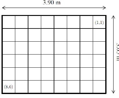
The adopted approach was to manually translate the custom target object through the measurement volume. The target was mounted on top of a substantial tripod (Manfrotto 161MK2) providing a stable support, minimising target occlusion from the cameras, and allowing for vertical translation of the target object. When scanning a plane the height of the tripod was fixed for all measurements in the plane thus ensuring that the measurements were co-planar to within the planarity of the laboratory floor (1mm deviation recorded by the laser tracker). A series of four vertical positions were considered, and at each height a total of 48 discrete points were measured, making 192 measurement positions in total. Figure 5 shows the eight by six grid measurement grid marked out on the ground plane to aid in sampling the measurement volume at approximately constant intervals.

Figure 5 - Grid used to guide acquisition

Custom software was written to obtain co-ordinated measurements from both tracking systems. Two datasets were collected, the first where the Vicon photogrammetry system was calibrated using the passive wand, while the second calibrated the system using the active wand (as discussed in section 2.2). The measurements were captured in four planes 0 ... 3 such that the data for plane 0 was collected at a height of 0.03 m while planes 1- 3 where captured at tripod height settings of 1.06 m, 1.80 m and 2.30 m respectively. At each measurement location 100 measurements were acquired by both systems.

3. Experimental results

3.1 Coordinate frame alignment

Since the measurements were acquired in different system coordinate frames, an alignment procedure was required prior to error analysis. Note that in the following analysis, the use of bar notation denotes a mean data point computed from 100 collected data points. A Vicon measurement, i, may be expressed in the coordinate frame of the laser tracker as follows:

s (3)

9 systems, the transformation parameters R, t and s may be recovered through minimisation of the cost function [26]:

e s 1 _{i 1} -(s ) (4)

where, || ||, denotes Euclidean distance. Through the inclusion of scale, s, this equation describes a more flexible transformation relating two corresponding point sets. In the following analysis it will be shown that the error vectors computed between the measurements have a particular structure. From our analysis it will be apparent that this structure is best explained by a difference in this scale factor. The analysis, therefore, proceeds in two parts. The first part considers the case where s = 1 which corresponds to processing the raw data produced by Vicon. Given a fixed scale constraint, Equation 4 is minimised as a function of R and t using the method described in [27]. The second part considers the more generic case where s is jointly estimated with the rigid body parameters using the minimisation described in [26].

Figure 6 - Error surfaces for each plane using passive wand, scale fixed

In accordance with the grid in Figure 5, the distance error at row, r, and column, c, between a Vicon and laser tracker measurement is calculated as follows:

10

3.2 Case I: Fixed Scale S = 1

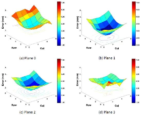
Error as a function of row and column for each layer is shown in Figure 6 for the passive wand and Figure 7 for the active wand. It was found that in general use of the system the errors at the edges of the volume were greater than those at the volume centre. This suggested that the error function would a have a lower value in the centre than the edges. This observation is depicted clearly in the passive wand dataset for planes 0 - 2 and to a lesser extent in plane 3. The error surfaces corresponding to the active wand display similar behaviour particularly in planes 1 and 2. The minimum, mean and maximum errors for each plane are shown in Table 2. Significantly, the errors resulting from the active wand are less than those obtained by calibrating using the passive wand for each plane. The maximum error across the dataset for the passive wand was 7.15 mm while the active wand resulted in a maximum of 4.03 mm. The minimum errors due to the active wand are uniformly sub-millimetre while those for the passive wand vary widely with the worst minimum error being 3.09 mm observed in plane 0. Based upon this data, a system operator could expect an overall mean error of 1.48 mm for the active wand and 3.95 mm for the passive wand.

Figure 7- Error surfaces for each plane using active wand where scale is fixed

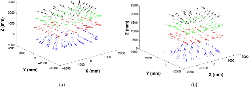
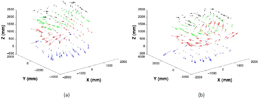
In order to visualise the spatial error distribution for each calibration artefact, Figure 8 shows a plot of the error vectors at each location. (The arrow heads point toward the true position). Interestingly, the direction of the error vectors for the passive wand are in the opposite direction to those associated with the active wand. Figure 8 (a) suggests that calibration with the passive wand results in the volume being contracted with respect to the true position of the object. The opposite is true in the case of the active wand where the volume is inflated relative to the true position. Estimation of the scale would bring the point clouds into closer alignment motivating the next section.

11 Wand Plane Min

(mm)

Mean (mm)

Max (mm)

Passive

0 3.09 4.89 7.15

1 0.93 3.32 5.51

2 1.67 3.43 4.99

3 2.99 4.16 6.21

Active

0 0.44 1.29 2.85

1 0.32 1.28 2.49

2 0.35 1.48 2.78

3 0.89 1.88 4.03

Table 2- Minimum, mean and maximum errors with scale fixed to unity

Figure 8-Error vectors with scale fixed (a) Passive Wand (b) Active Wand

3.3 Case II: Scale Estimation

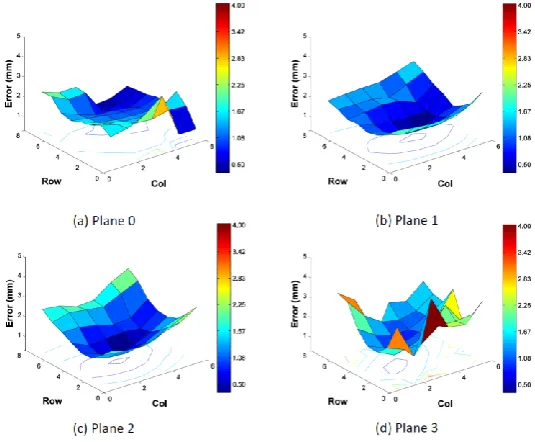
12 Figure 9 - Error surfaces for each plane using passive wand where scale has been estimated

Figure 10 - Error surfaces for each layer using active wand where scale has been estimated

13 obtained by multiplication of the fixed scale case (section 3.2) by the scale factor, s. Therefore, in both cases there is little change in these values.

Wand Plane Min (mm)

Mean (mm)

Max (mm)

Passive

0 0.06 0.69 2.36

1 0.09 0.37 0.89

2 0.16 0.53 1.32

3 0.26 0.76 2.71

Active

0 0.06 0.55 2.11

1 0.03 0.31 0.58

2 0.05 0.44 1.09

3 0.09 0.73 2.39

Table 3- Minimum, mean and maximum errors with scale estimated

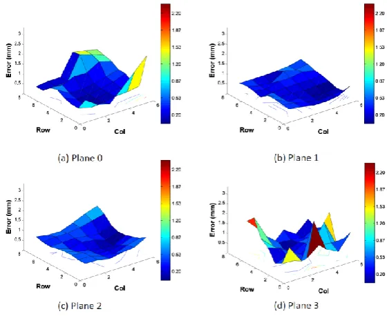
Figure 11 Error vectors with scale estimated (a) Passive Wand (b) Active Wand

4. Discussion

14 the measurement process itself introduces error and thus it may not be possible to entirely attribute scaling error to this effect. Significantly when the scale factor is known, the errors displayed in Table 3 are of a similar magnitude with the average errors becoming 0.59 mm for the passive wand and 0.51 mm for the active wand. Adjustment of the scale factor thus results in a significant reduction in error and makes the difference in calibration artefact type negligible. Direct comparison of current findings with previous studies is made difficult due to differences in hardware and the relative size of the measurement volumes. As discussed in the introduction, most previous studies have concentrated on relatively small measurement volumes consistent with small biomechanical sample measurements. The accuracy with which the centre of the marker is estimated is dependent upon the number of pixels representing the marker in the image. Clearly the greater the number of pixels, the more accurately the shape is captured leading to less error in measuring the centre. Increasing the number of pixels may be achieved by increasing the resolution of the camera or reducing the distance between the marker and camera. Overall the precision of the measurements in each coordinate was less than 10 µm therefore indicating that the photogrammetry system was precise but inaccurate. The systematic nature of the inaccuracy may be mitigated through improving the calibration of the system.

End users of photogrammetry systems for all precision measurement applications should be aware that the magnitude of error associated with measurements is a function of multiple variables including volume size, camera resolution and volume location, as well as calibration approach. General guidance would indicate it would always be prudent to conduct appropriate tests to ensure that the measurement error is within acceptable bounds for the application concerned. Follow up work shall involve the manufacture of a high accuracy calibration artefact to verify the conclusions regarding scale drawn in the analysis.

5. Conclusion

An experimental characterisation of the static positional accuracy and precision of a Vicon T160 photogrammetry system using a high accuracy laser tracker has been presented. The motivation for the study arose through empirical observations of large errors (up to 10 mm) when using robotic measurement systems whose positions were tracked using photogrammetry in a measurement volume of approximately 100 m3_{. Precision robotic positioning and control often demands sub-millimetre} accuracy motivating significant improvements in the absolute error quantification in this measurement application.

The absolute error of the photogrammetry system was evaluated through simultaneously tracking a target scanned through a 3.9 x 3.05 x 2.3 m3 _{measurement volume (27 m}3_{), and comparing the} computed position with the position from the laser tracker. To enable the simultaneous measurements to be undertaken with these two quite different systems required the construction of a custom target. The final target object was mounted on a tripod and measured at each point of a grid of size 8 × 6 and moved through four height settings to generate a set of 192 measurement points. When processing raw data from the photogrammetry system, an error surface was obtained (for a fixed height setting) which displayed lower error in the central region of the volume than the edges - this confirmed empirical observations. It was found that unscaled data mean errors of 1.48 mm and 3.95 mm were obtained for the active and passive techniques respectively (with a maximum observed errors of 4.03mm and 7.15 mm respectively). Through close inspection of our initial experimental findings it became clear that the measurements from both calibration approaches were related by an unknown scale factor. Through estimation and subsequent application of this scale factor, the overall system errors were reduced to 0.51 mm and 0.59 mm for active and passive calibration artefacts respectively.

15 The approach outlined in this study has enabled a rigorous approach to be established for the calibration of photogrammetry systems for large volume measurement applications (particularly relevant to robotic tracking applications), and additionally provided insight into improved calibration procedures to promote increased measurement accuracy.

6. References

[1] Vicon. 2015. Vicon. [ONLINE] Available at: http://www.vicon.com/ . [Accessed 10 February 15].

[2] Qualisys Motion Capture Systems. 2015. Qualisys. [ONLINE] Available at:

http://www.qualisys.com/ . [Accessed 10 February 15].

[3] OptiTrack. 2015. OptiTrack. [ONLINE] Available at:https://www.naturalpoint.com/optitrack/. [Accessed 10 February 15].

[4] Cappozzo A 1984 Gait analysis methodology Human Movement Science pp 27–50

[5] Bregler C 2007 Motion capture technology for entertainment [in the spotlight] Signal Processing Magazine, IEEE pp 160–158

[6] Michael N, Mellinger D, Lindsey Q and Kumar V 2010 The grasp multiple micro-UAV testbed, Robotics & Automation Magazine, IEEE pp 56–65

[7] Meier L, Tanskanen P, Heng L, Lee G H, Fraundorfer F and Pollefeys M 2012 Pixhawk: A micro aerial vehicle design for autonomous flight using onboard computer vision, Autonomous Robots pp 21–39

[8] Dobie G, Summan R, MacLeod C and Pierce S, Visual odometry and image mosaicing for NDE, NDT & E International

[9] Kwartowitz DM, Miga, MI, Herrell SD and Galloway RL 2009 Towards image guided robotic surgery: multi-arm tracking through hybrid localization International journal of computer assisted radiology and surgery pp 281-286.

[10] Chiari L, Croce UD, Leardini A and Cappozzo A 2005 A Human movement analysis using stereophotogrammetry - Part 2: Instrumental errors, Gait and Posture pp 197–211

[11] Yang PF, Sanno M, Brüggemann GP and Rittweger J 2012 Evaluation of the performance of a motion capture system for small displacement recording and a discussion for its application potential in bone deformation in vivo measurements, Proceedings of the Institution of Mechanical Engineers, Part H: Journal of Engineering in Medicine pp 838–847

[12] Liu H, Holt C, Evans S 2007 Accuracy and repeatability of an optical motion analysis system for measuring small deformations of biological tissues Journal of biomechanics pp 210–214 [13] Windolf M, Gotzen N, Morlock M 2008 Systematic accuracy and precision analysis of video

motion capturing systems - exemplified on the Vicon-460 system Journal of biomechanics pp 2776–2780

[14] Dobie G, Summan R, Pierce S, Galbraith W and Hayward G 2011 A Non-Contact Ultrasonic Platform for Structural Inspection IEEE Sensors Journal pp 2458-2468

[15] Mineo C, Herbert D, Morozov M, Pierce SG, Nicholson PI and Cooper I 2012 Robotic Non-Destructive Inspection 51st Annual Conference of the British Institute for Non-Destructive Testing

[16] Ehara Y, Fujimoto H, Miyazaki S, Mochimaru M, Tanaka S and Yamamoto S 1997 Comparison of the performance of 3D camera systems II, Gait & Posture 5 pp 251–255 [17] Richards JG 1999 The measurement of human motion: A comparison of commercially

available systems, Human Movement Science pp 589–602

[18] Borghese NA, Cerveri P and Rigiroli P 2001 A fast method for calibrating video-based motion analysers using only a rigid bar Medical and Biological Engineering and Computing pp 76–81 [19] Geodetic VStars. 2015. Geodetic Systems inc. [ONLINE] Available at:

16 [20] GOM. 2015. ATOS Professional: GOM. [ONLINE] Available at:

http://www.gom.com/3dsoftware/atos-professional.html. [Accessed 10 February 15]

[21] Durrant-Whyte, H., & Bailey, T. (2006). Simultaneous localization and mapping: part I.

Robotics & Automation Magazine, IEEE, 13(2), 99-110. [22] Leica-Geosystems URL http://www.leica-geosystems.com.

[23] Hartley R and Zisserman A 2000 Multiple View Geometry in Computer Vision, vol. 2, Cambridge Univ Press

[24] L. G. M. Products, Leica Absolute Tracker: ASME B89.4.19 Specifications [25] BS ISO 3290-1: 2008 Rolling bearings Balls. Part 1. Steel balls

[26] Umeyama S 1991 Least-squares estimation of transformation parameters between two point patterns IEEE Transactions on Pattern Analysis and Machine Intelligence pp 376–380