A tree formulation for signaling games

City, University of London Institutional Repository

Citation

:

This is the unspecified version of the paper.

This version of the publication may differ from the final published

version.

Permanent repository link: http://openaccess.city.ac.uk/1455/

Link to published version

:

Copyright and reuse:

City Research Online aims to make research

outputs of City, University of London available to a wider audience.

Copyright and Moral Rights remain with the author(s) and/or copyright

holders. URLs from City Research Online may be freely distributed and

linked to.

City Research Online: http://openaccess.city.ac.uk/ [email protected]

Department of Economics

A Tree Formulation for Signaling Games

Xeni Dassiou

D. Glycopantis

City University London

Department of Economics

Discussion Paper Series

No. 11/07

1 _{Department of Economics, City University London, Social Sciences Bldg, Northampton Square, London EC1V 0HB, UK.}

Emai

A tree formulation for signaling games

X. Dassiou1 and D. Glycopantis2

1 _{Department of Economics, City University, Northampton Square, London EC1V 0HB,}

UK (e-mail: [email protected])

2 _{Department of Economics, City University, Northampton Square, London EC1V 0HB,}

UK (e-mail: [email protected])

∗_{We would like to thank Dr. Angelos Dassios for his comments. Of course responsibility for all} short-comings stays with the authors.

Correspondence to: X. Dassiou

A tree formulation for signaling games

Abstract. We provide a detailed presentation and complete analysis of the sender/receiver

Lewis signaling game using a game theory extensive form, decision tree formulation. The analysis employs well established game theory ideas and concepts. We establish the ex-istence of four perfect Bayesian equilibria in this game. We explain which equilibrium is the most likely to prevail. Our explanation provides an essential step for understanding the formation of a language convention. Further, we discuss the informational content of such signals and calibrate a more detailed definition of a true (“correct”) signal in terms of the payoffs of the sender and the receiver.

Keywords and Phrases: Signals and signaling games, Actions, States of nature,

Language convention, Rational expectations equilibrium, Information set, Games with imperfect information, Nash equilibrium, Perfect Bayesian equilibrium, Beliefs updating. .

1

Introduction

The philosopher, Professor D. Lewis (1969), writing on the origins and process of formation of language discusses signaling games between a sender, who sends a signal, and its receiver. In the Lewis formulation the sender is aware of the state of the world, but the receiver is not. There are a number of alternative states and nature chooses one at random, i.e. with a certain probability. Once the sender knows the state chosen, there are various signals that he can use. There is a number of alternative actions that a receiver can take in response to the signal received.

Following the specific actions of the sender and the receiver there are payoffs awarded to both of them. These rewards express, for example, the utilities or money, obtained from the combination of their actions. We note in particular the games of common interest in which a resolution leads to optimal payoffs for both actors as noted by Skyrms (2010).

However this type of analysis is not always complete. Notably there is little discussion of the case where the action of the receiver may be appropriate to the state of nature even if the signal sent is not. There is no discussion of what happens to the payoffs of the two agents when this is the case. Lewis makes an attempt to discuss what constitutes “true” and “untrue” signals and responses in a signaling system. We discuss these issues below.

1 INTRODUCTION ₃

“The helper gestures as he does because he expects theDto respond as he does, and the D responds as he does because he expects the helper to gesture as he does.” (p. 127).

This means that the expectations of the actors are self-fulfilling and they both receive their optimal payoffs. One can borrow concepts and approaches from neighbouring disciplines, notably game theory and economics. They can provide a formal interpretation of the outcome in terms of existing concepts in those areas (rational expectations, self-fulfilling prophesies) using a fixed point theorem from mathematics. We return to this point below. Of course this is not always the case. A deviation from this rule, perhaps based on lack of trust, could lead to one or both of them getting inferior payoffs. The issue is to investigate whether a “correct” interpretation of the signals is possible which would lead to such an equilibrium position being reached. In such a situation no one would wish to independently change his action if all the information was revealed and moreover the payoffs would be optimal.

More formally, in a signaling problem there are alternative states of natureT1, T2,.., Ti, ..., Tn.

These are observed, let us say, by one sender, who will send a signal concerning the in-formation received, i.e. the state chosen by nature. The receiver then has to choose an action without knowing the state of nature. The sender compiles a set of alternative signals s1, s2, ..., sj, ...sm using a function FH : {Ti} → {sj}. In other words, FH is the

function that translates the states of nature into communicated signals. In order to be able to identify eventually the state with a signal we requirem≥n.

Clearly there will be _(mm₋!_n)! possible signaling systems, that is alternativeFH’s functions.

Suppose next that the set of actions available to Darer1, r2, ..., rk...rn. Given a signal sj

we define FD :

n rk/(_sj)

o

→ {Ti}.The function FD is designed to translate actions based

on a signal received into a maximum payoff for D. The signal received and the action chosen combined with the state of nature implied by FD should lead to D’s maximum

payoff. (FH, FD) will be called a signaling convention. It is of course true that differently

designed signaling systems combined with an association between actions and states of nature could produce the same result. I.e., an alternative convention (F′

H, FD′ ) has the

same outcome.

In the analysis above truthfulness in signaling is viewed as a signal that allows D to correctly identify the state of nature. We also pointed out that different functions FH

may qualify.

Here we move one step further and consider truthfulness as a signal that leads to bothH

and D receiving their maximum payoffs. The reason for this stricter definition is that D

might correctly guess the state of nature althoughH sends the wrong signal. In this case

H does not receive a high payoff.

Nature

the helper the helper 1/2

1

1 0₀ 00

0 0 1 1 1 0 1 ₂ 0 0 0 1

The general formulation of the game η1 η3 η2 η4 r′ r′ l l L I2 I1

1−p l′

q

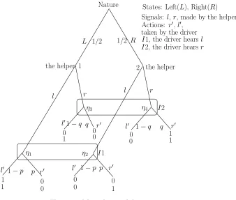
States: Left(L), Right(R) Signals: l,r, made by the helper Actions: r′,l′,

I2, the driver hearsr I1, the driver hearsl taken by the driver

r′ l′ r r R 1/2 p p

1−q

1−p l′₁₋q q _r′

l′

Figure 1

2

A game tree approach

We introduce here the game theoretic analysis by concentrating on aH/Dexample which is a detailed elaboration of the discussion by Lewis. The analysis is in terms of an appro-priate, extensive form, tree formulation of a non-cooperative, signaling game. The set-up is one with asymmetric information. The player who is informed, i.e. the helper here, moves first to signal, truthfully or not, his information to the receiver, i.e. the driver. The relevant concepts and ideas are discussed briefly, (see, for example, Binmore (1992), Osborne and Rubinstein (1994)).

Figure 1 gives the simple tree formulation of our game. There are two equally probable states of nature, a truck must move Left (L) or Right (R), each with probability 1/2, and two signals,l and r, that can be made byH. On the other hand,D can choose from two alternative actions, l′ _{and r}′_{, having heard the signal but without knowing the state of}

nature. Therefore she does not know whether he is at nodeη1 orη2 of information set I1,

when he hears l neither if he is at node η3 or η4 of information set I2, when he hears r.

A play of the game starts from the initial node to a terminal point, where the game ends. The payoffs at the terminal nodes refer to the payoffs ofH, the upper number, and ofD, the lower number.

In the information setI1, enclosed by a parallelogram, player D does not know whether she is at nodes η1 or η2.Similarly when D enters information setI2, she does not know

2 A GAME TREE APPROACH ₅

the nodes of an information set are identical.

Pure strategies are rules that tell each agent what action to choose from each information set. They can be played with probabilities as mixed strategies. The pure strategies of

H are (lr;ll, rl, rr) emanating from points 1 and 2, (L and R respectively). The pure strategies of D are (l′_r′_{, l}′_l′_{, r}′_l′_{, r}′_r′_{) from information sets I1 and I2 respectively. For}

example l′_r′ _{means that D plays l}′ _{from information set I1 and r}′ _{from information set} I2.

D’s mixed strategy is (l′_l′_{, z}

1;l′r′, z2;r′l′, z3;r′r′, z4), where, for example, l′r′ means that

D plays l′ _{from information set I1 and r}′ _{from information set I2 with probability z}

2.

Of course zi ≥0 for i= 1,2,3,4 and they sum up to 1. The mixed strategies of H are

analogously defined.

We are looking at the idea of an equilibrium in such a game. The general proof of existence of an equilibrium in the set-up of abstract mathematical spaces is based on the concept of the fixed point theorem. Under appropriate technical assumptions, a function from one space to itself has fixed point, i.e. an element of the domain which maps onto itself. There are a number of such theorems, depending on the generality of the mathematical conditions imposed. Of course in particular explicit examples, like the one we are investigating, we do not have to go through a formal proof of existence. We can simply check directly that a set strategies satisfy the properties which characterize an equilibrium.

First, we consider the well known and widely used idea of a Nash equilibrium (NE). A number of players with their own individual sets of (mixed) strategies are given and payoffs depend on everybody’s action. A set of (mixed) strategies, one for each player is a NE, if for each player his choice is a best response, in terms of payoff, given the other agent’s action.

The payoffs show that when H reveals the “correct” signal and the correct action (the one corresponding to the actual state of the world) byD follows, then they both receive a payoff of 1. IfH communicates an incorrect signal and this leads to an incorrect action by D, then both players get 0. If H chooses an incorrect signal andD reacts counter to the signal indicated then D gets 1 for performing the correct action butH ends up with zero.

We set the probability that D plays l′ _{in I1 as z}

1 +z2 = 1−p, while z3 +z4 = p is

the probability that D plays r′ _{in I1, z}

1 +z3 = 1−q is the probability that D plays

l′ _{in I2 and finally z}

2 +z4 = q is the probability that D plays r′ in I2. We note that

1−p, pand 1−q, q, shown in Figure 1, can be also thought of as behavioural strategies describing howDchooses between the action from an information set. We shall return to this immediately below. At this stage 1−p, pand 1−q, qthe specific way the probabilities

zi are combined.

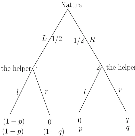
We can use the probabilities attached to the choices from I1 and I2, described in Figure 1, to fold the tree up, as seen in Figure 2, given the choices of the strategies and their probabilities and can calculate the expected payoffs of H and D from left to right of the new terminal nodes as (1−p,1−p), (0,1−q), (0, p) and (q, q).We emphasize that these are expected payoffs of the two agents. We shall use this information in considering the possibilities for NE.

Nature

1/2

the helper 1

2

the helper

(1

−

p

)

0

0

l

r

l

L

_R

(1

−

p

)

(1

−

q

)

p

q

q

1/2

r

Given the driver’s strategies in the previous figure,

the tree folds up as above.

Figure 2

distributions on the nodes of each information set, and consistent with these a set of beliefs which attract a probability distribution to the nodes of each information set. Consistency requires that the decision from an information set is optimal given the particular player’s beliefs about the nodes of this set and the available information. If the optimal play of the game enters an information set the updating of beliefs must be Bayesian. Otherwise appropriate beliefs are assigned arbitrarily to the nodes of the set. The assignment of beliefs is a characteristic feature of a PBE.

The proof of existence of a PBE is also based on a fixed point theorem. In our explicit example, we can simply check directly that a set of behavioural strategies satisfy the properties which characterize an equilibrium.

The player uses independent distributions to choose between the action of the information sets. For example she spins a wheel to decide betweenl′ _andr′ _{inI1 and a wheel divided}

differently for choosing when she is in I2. The same principle applies if information sets are singletons, i.e. consist of the single point. This applies to sets 1 and 2 belonging to

H. In order to avoid introduce too much notation, we use again 1−p, pand 1−q, q, for the behavioural strategies in I1 andI2 respectively. ForH’s behavioural strategies at 1 and 2 we shall use the independent distributions 1−y, y and 1−w, w, respectively for choosing between land r.

2 A GAME TREE APPROACH ₇

Our detailed presentation and analysis of the model show that there exist more than one equilibria. This forces the analysis into a further argument for the choice of the most reasonably expected one.

Finally we note that the structure of our model is such that there is a complete, one-to-one correspondence between NE and PBE. The reason is because all the NE here are in pure strategies. Such strategies define behavioural strategies as well. On the other hand it is part of the definition of the richer PBE to consider beliefs and their updating, and their consistency with strategies.

2.1 Lack of a NE or a PBE

We show here that for {0 < p <1, q arbitrary} ∪ {0 < q < 1, p arbitrary}, there is no NE and also no PBE either. We refer to Figure 1 and in particular to Figure 2.

We consider the possibility of a NE. The pair of probabilities (p, q) are seen as implied directly from the zis of mixed strategies, which has been shown above. First we consider

the case{0< p <1, q arbitrary}. We point out that, as it is shown in the Appendix, any such pair p, q can be realized by a set of feasible zis.

We inspect Figure 2. We consider as a candidate for a NE, player H to play lr (since {0 < 1−p < 1, q ≥ 0)}; but then D will respond with p = 0, q = 1 which does not belong to the set of strategies above. IfH was to playllthenDwould respond again with

p= 0, q = 1, forcing H to play lr to become better off. Finally ifH was to play rl orrr

then D would respond with p = 0, q = 1, forcing H to respond with lr. Hence none of these strategies forH would lead to a Nash solution. Furthermore no mixed strategy for

H would lead to NE because D will use againp= 0 and q= 1.

We now consider {0 < q < 1, parbitrary}. Again, as it is shown in the Appendix, any such pair p, q can be realized by a set of feasible zis. We inspect again Figure 2. We

consider as a candidate for a NE, player H to play lr (since {0 < q < 1, p ≥ 0)}; but then D will respond with p = 0, q = 1 which does not belong to the set of strategies above. If H was to play ll then D would respond again withp = 0, q = 1 forcing H to change his strategy to lr. Finally if H was to play rl orrr then D would respond again with p = 0, q = 1, which is outside the set of strategies we are considering, forcing H

to respond with lr. Hence none of these strategies for H would lead to a Nash solution. Furthermore no mixed strategy for H would lead to NE becauseD will use again p= 0 and q= 1 forcingD to playlr.

Next we consider the possibility of a PBE where the distributions on the choices between the information set are taken to be independent from each other. We consider the case {0 < p < 1, q arbitrary}. Suppose that H has chosen some pair of distributions (y, w). The pairs (p, q) and (y, w) are not optimal. H will want to set y = 0 and then D will respond with p= 1.

An analogous argument shows that for{0< q <1, parbitrary}, and independently taken distributions, the pairs (p, q) and (y, w) are not optimal.

2.2 The calculation of NEs and the PBEs

(0, 0)

(1, 1) (0, 1)

(1, 0)

the various cases for a PBE:

q

p

(

p

= 1

, q

= 1), (

p

= 0

, q

= 0),(

p

= 1

, q

= 0),(

p

= 0

, q

= 1).

Figure 3

effect, a reaction function is formed. If each player optimizes believing, (prophesying), a particular strategy for the other, and the outcome is that there is no reason for anybody to feel they have predicted wrongly, then we a have an equilibrium which has been obtained rationally. The confirmation of the predictions takes places where the reaction functions intersect.

The analysis in the previous subsection implies we are only left to consider the four corner cases (p = 0, q = 1), (p = 1, q = 1), (p = 0, q = 0), and (p = 1, q = 0) in Figure 3. We shall show that they are all PBEs. However there is only one which can reasonably be expected to prevail. In order to obtain this we need to invoke an extra argument over and above the conditions for a NE or a PBE.

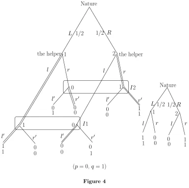
Case 1: p= 0, q= 1 This is shown in Figure 4. These probabilities imply z3+z4 = 0

and z2+z4 = 1. Hence z2 = 1 and D decides to play l′r′ and the tree folds up into the

smaller one in Figure 4. The best response for H is to play play l from L and r from

R, hence the strategy lr. We write these pair of strategies as (lr, l′_r′_{). to this, the best}

response byDis to play l′_r′_{. Hence the pair of pure strategies (lr; l}′_r′_{) form a NE.}

Next we turn our attention to the existence of a PBE. We consider the set of pairs of behaviour strategies ofH and D given by ((l, 1;r, 1); (l′_{, 1; r}′_{, 1)), where for example}

(l, 1;r,1) means thatH at point 1 playsl with probability 1 and at point 2 he choosesr

with probability 1. It is straightforward to see that these pairs are optimal in the sense of being a best response by an agent to the behavioural strategy of the other.

The calculations, through Bayesian updating, of the conditional probabilities, (beliefs), attached to the nodes of I1 and I2 is based on these strategies.

Consider information setI1.The left-hand-side node is denoted byη1 and the

right-hand-side one by η2. We wish to calculate the beliefs attached to these nodes byD. Using the

Bayesian formula for updating beliefs, (see for example Glycopantis at al., 2003), we can calculate these conditional probabilities. We know that I1 is entered only if H plays l. Hence

P r(n1/l) = P r(l/n1)×P r(n1)

P r(l/n1)×P r(n1) +P r(l/n2)×P r(n2)

= 1×1/2

1×1/2 + 1×0 = 1 (1)

2 A GAME TREE APPROACH ₉

Nature

the helper

1/2

1

1

0

₀

0

0

0

0

0

₀

1

₁

1

0

1

1

1

0

0

1

2

0

Nature

0

1

1

r

0

0

0

1/2

1

1

l

r

l

r

l

l

l

l

L

R

I

1

I

2

L

R

(

p

= 0,

q

= 1)

r

the helper

1/2

1/2

r

r

r

l

_l

r

1

₂

Figure 4

On the other handI2 is entered only if H plays r. The left-hand-side node is denoted by

η3 and the right-hand-side one byη4. Hence

P r(n3/r) =

P r(r/n3)×P r(n3)

P r(r/n3)×P r(n3) +P r(r/n4)×P r(n4)

= 1×0

1×0 + 1×1/2 = 0 (2)

Similarly we obtain the conditional probabilityP r(n4/r) = 1

Finally, the optimality of the strategies given these beliefs can be easily checked. Hence ((l, 1;r, 1); (l′_{, 1; r}′_{, 1)) a PBE. Of course it is connected to the NE because pure}

strategies imply that the implied behavioural strategies played with probability 1 from the relevant information set.

The expected payoffs are calculated as follows. Htells the truth always and gets expected payoff 1/2×1 +1/2×1=1. Dalways makes the correct move and also gets expected payoff 1/2×1 +1/2×1=1.

We can provide some more explanation with respect to the expected payoffs. As expected earlier a folded up tree can be obtained and now we are using the optimal strategies ofH

Nature

the helper the helper 1/2

l

1 0₀ 00 0

0 0₀

1 1

1 2

1 0

0 1

0

0

Nature

1/2

1 2

0 1 1/2

0 0 0

1 0

0

1/2 I2

I1 r′

l′ l′ l′

l′

l r l r

L R

R r

l r

r′

r′ r′

L 1

1

(p= 1,q= 0) 1

Figure 5

point 1 andr from point 2. The NE and PBE follow.

Case 2: p = 1, q = 0 This is shown in Figure 5. Hence z3+z4 = 1 and z2+z4 = 0

implying z3 = 1. D decides to play r′l′ and the full tree folds up into the smaller one in

Figure 5. A best response byH is to playrland to this a best response ofDisr′_l′_{. Hence}

the pair of pure strategies (rl; r′_l′_{) form a NE.}

With respect to the existence of a PBE, we consider the set of pairs behaviour strategies of H and D given by ((r, 1;l, 1); (r′_{, 1; l}′_{, 1)). It is easy to see that these pairs are}

optimal. Namely, they are a best response by an agent to the behavioural strategy of the other.

The calculations, through Bayesian updating, of the conditional probabilities, (beliefs), attached to the nodes I1 and I2 are based on these strategies. The formulae used are analogous to the ones in Case 1 and the values are shown in Figure 5. The optimality of the strategies given these beliefs can be easily checked. Hence ((r, 1;l, 1); (r′_{, 1; l}′_{, 1))}

is a PBE.

2 A GAME TREE APPROACH ₁₁

1

1 0

0

Nature

the helper the helper 1/2 1/2 0 0 0 0 0

0 ₀0

1 0 1 1 2 0 1-x 1/2 1/2 x 0 0 I2 I1 l r l′ l′

l′ l′

L R

(p= 0,q= 0) r′ _r′

r′ r l r l 1 1 2R 1/2 1/2 1

r′ _Nature

0 1 r L 1 l 1 Figure 6

indicates, and ends with an expected payoff of 1. In the folded up tree of Figure 5 it is clear theH must use r from point 1 and lfrom point 2. The NE and PBE follow. We can provide some more detailed explanation with respect to the expected payoffs. In the folded tree, given D’s choices, a payoff of 0 is indicated for H irrespective of his strategies. The beliefs 0 and 1 inI1 are consistent withDplayingr′_{. This gives expected}

payoff 0×0 + 1×1 = 1 while playingl′ _{gives 0×1 + 1×0 = 0. Hence actionr}′ _{is preferable}

to l′_.

Also, the beliefs 1 and 0 inI2 are consistent with Dplayingl′_{. This gives expected payoff}

1×1 + 0×0 = 1 while playingr′ _{gives 1×0 + 0×1 = 0. Hence actionl}′ _{is preferable to} r′_.

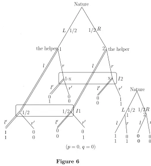
Case 3: p = 0, q = 0 This is shown in Figure 6. These probabilities imply z3+z4 = 0

andz2+z4 = 0. Hencez1= 1 andDdecides to playl′l′ and the full tree folds up into the

smaller one in Figure 6. A best response forH is to playll and to this a best response of

D isl′_l′_{. Hence the pair of pure strategies (ll; l}′_l′_{) form a NE.}

With respect to the existence of a PBE, we consider the set of behaviour strategies of H

and D given by ((l, 1;l, 1); (l′_{, 1; l}′_{, 1)). It is again straightforward to see that these}

pairs are optimal in the sense of being a best response by an agent to the behavioural strategy of the other.

1/2 1/2

x 1−x

Nature

the helper the helper 1/2 1/2

1

1 0₀

0 0

0

0 ₀0

1 0

1

1 2

0

0

0 00 10 11 1/2 1/2

Nature L

L _R

r l r

l r l r

l I1

I2

l′ l′

(p= 1,q= 1)

R

r′ r′

r′ r′ l′ _l′

2 1

1 1

Figure 7

to the ones in Case 1 and the values are shown in Figure 6. We note that the game never enters I2, and hence 1−x, x are arbitrary. In the Bayesian formula for updating, since

P r(η3) =P r(η4) = 0 we obtain 0/0.

The optimality of the strategies given the beliefs in I1 can be easily checked. Hence

((l, 1;l, 1); (l′_{, 1; l}′_{, 1)) is a PBE.}

The expected payoffs are calculated as follows. Halways plays l. Hence he tells the truth once with probability 1/2 and gets expected payoff 1/2×1. D always plays l′ _{i.e. she}

makes the correct move once and gets expected payoff 1/2×1. In the folded up tree of Figure 6 it is clear theH must uselfrom point 1 and he can alsol from point 2. The NE and PBE follow.

It is important to note that in this equilibriumthe informational content of H’s signal is zero and hence the (updated) beliefs of D inI1 are identical to the prior of the state of nature. Professor Lewis refers in his book to inadmissible signals. The signal here which conveys no information could be considered as an inadmissible one.

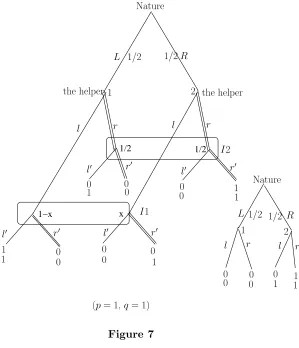
Case 4: p= 1, q= 1 This is shown in Figure 7. These probabilities implyz3+z4= 1 and

z2 +z4 = 1. Hence z4 = 1 and D decides to play r′r′ and the full tree folds up into the

smaller one in Figure 7. A best response forH is to playrr and to this a best response of

D isr′_r′_{. Hence the pair of pure strategies (rr; r}′_r′_{) form a NE.}

2 A GAME TREE APPROACH ₁₃

and D given by ((r, 1;r, 1); (r′_{, 1; r}′_{, 1)). It is again straightforward to see that these}

pairs are optimal in the sense of being a best response by an agent to the behavioural strategy of the other.

The calculations, through Bayesian updating, of the conditional probabilities, (beliefs), attached to the nodes I2 are based on these strategies. The formulae used are analogous to the ones in Case 1 and the values are shown in Figure 7. The game never enters I1, and hence 1−x, x are arbitrary. In the Bayesian formula for updating, since P r(η1) =

P r(η2) = 0 we obtain 0/0.

The optimality of the strategies given the beliefs in I2 can be easily checked. Hence

((r, 1;r, 1); (r′_{, 1; r}′_{, 1)) is a PBE.}

The expected payoffs are calculated as follows. H always plays r. Hence she tells the truth once with probability 1/2 and gets expected payoff 1/2×1. D always plays r′ _i.e.

she makes the correct move once and gets expected payoff 1/2×1. In the folded up tree of Figure 7 it is clear thatH must user from point 2 and he can also use r from point 1. The NE and PBE follow.

Again, the informational content of H’s signal is zero in this Bayesian equilibrium.

It is important to note that also in this equilibriumthe informational content ofH’s signal is zero and hence the (updated) beliefs ofDinI1 are identical to the prior of the state of nature.

2.3 Comparing equilibria

Examining the four equilibria established above, we see that we have an information revelation problem. It is only in Case 1, where p = 0 and q = 1 that the signals of H

reveal to Dthe true state of the nature. In the Case 2, where p= 1 andq= 0, player H

always misreports the state and Dresponds by doing exactly the opposite of what she is told to do. While one should stress that this also is a perfect equilibrium for the game, it does implies zero expected payoff forH. He is punished for lying.

In the equilibria of Cases 3 and 4 player H’s signals do not reveal anything about the state of the nature and the driver D sets her expectations in accordance with the prior probabilities. The resulting, equilibrium expected payoff forH is inferior to that when he tells the truth.

Both players know that inconsistent announcements by H will lead to wasteful outcomes that will hurt him. Hence in such a context we have a truthful announcement. This can result from pre-play, “cheap talk”, exhanges between the players, in which it was agreed that the message sent by the sender will be truthful. (Binmore (1992, 2007), Rasmusen, 2007, Barrett, 2009). The incentives ofH andDare compatible. PlayerDcan reasonably expect, and correctly guess, thatH has an interest to observe the agreement and tell the truth. She comes to this conclusion on the basis of the structures of the payoffs, and thus uses an extra argument for choosing among the four PBEs. This is over and above the arguments which establish equilibrium strategies.

The equilibrium in Case 1 is the most likely to prevail. H knows that if he plays l only when he sees L and r only when he sees R, then D will prefer to play l′_r′ _{rather than,}

for example,r′_l′_{.This means that it is in the interests ofH for his signaling actions to be}

Of course, in deciding among the four PBEs examined above, H must find a way to communicate to D that he intends to do so. Clearly this is done on the basis of the expected payoff of the sender of the signal. Dwill rightly assume that H will want to do the best for herself in terms of payoffs and thus playlr.

Therefore we can define what is meant by “truth” and a true signal. In our example, if the convention is set as the one wherer corresponds toRandlcorresponds toLthen any other signaling system used is punishing at least one of the agents with a lower payoff, even if it results to a possible PBE. We return to this point in the following section.

3

Further discussion and conclusions

3.1 Discovering and updating the informational content of signals

We try to place, briefly, our analysis in a wider context of the literature. Skyrms (1996) follows Lewis’s work and develops, in effect, the dynamics of repeated games. He explains how individuals can converge to a common convention setting that indicates which signal is to be sent in a particular situation, as well as the receiver’s action for each type of signal communicated by the sender.

In a later article, Skyrms (2010) stresses the importance of the informational content of transmitted signals in updating beliefs. Nature chooses the state and then sends signals to intermediary receivers (senders). They can convey the information received to other agents through actions in the form of communicated signals. The informational content of signals alters the prior probabilities of states, as a result of the receiver updating his/her beliefs. This updating that takes place relative to the initial prior probability of a state of nature determines the informational content carried by a signal. Intuitively, the lower the prior probability, the higher the informational content of an accurate signal, i.e. one that is more likely to be representative of the true state of nature.

In the Lewis signaling game the sender and the receiver learn how to play through experi-encing successes and failures in repeated rounds of the game. This leads to the evolution of a sigaling game, e.g. a “convention”. This signaling system evolves through reinforcement learning. It takes the form of rewards for correct choices by the receiver for both of the agents. The accumulation of these rewards leads to the updating by the receiver of the probabilities of the states of nature.

In Barrett’s article instead of through rewards, updating takes the form of adding balls to the sender’s urn of the correct signal, i.e. when the receiver’s action matches the actual, given state of the world. Balls are also added to the receiver’s corresponding action urn. Originally the balls in the urns correspond to the prior probabilities of the different states of nature. The adding of balls to the signal and action urns changes the relative proportion of balls in each urn and we have a process of continuous updating. This results in the formation of a matching law (Herrnstein, 1970).

3 FURTHER DISCUSSION AND CONCLUSIONS ₁₅

repetitive signal, concerning the probability of a specific state of nature,Ti.

Consider, for example, the formula

a= Pr(T i|C, a0, K) =

a₀ a0+λC(1−a0)

.

aindicates the informational content of the signal for a given state of nature. It has prior

a0, starting time “0”, a running time ofKperiods, a learning speed convergence parameter

0< λ <1,and a cumulative experience cardinality C, whereC =

K−1

X

j=0

hj;hj = 1 for each

period the signal is correct and hj = 0 when it is not.

This updating formula is in effect an extension of the Bayesian updating used in this paper, and could be more appropriate for a mathematical formulation of a repeated game. This dynamic formula in which α tends to 1 could be considered as a background to the completed process in which our presentation rests.

One can note that there may be cases where there is plentiful information about the states in the signals, but zero information in the act that will be chosen by its receiver.

This applies if the receiver always performs the same act irrespective of the signal. This case has been explored in depth in the economics literature of herding behaviour.

As an example of this, in the formation of investment cascades there is no longer rein-forcement learning. The actions performed by the receiver of a private signal (for example a signal whether or not to invest in a particular project which may be either a good (profitable) or bad (loss making) investment, is no longer an indicator of her private information. Instead, a potential investor follows the same act as his/her predecessors irrespective of what his/her private information indicates. (See, for example, Bannerjee (1992), Bikhchandani et al. (1992), Choi et al. (2000), Welch (1992) among many other authors on this type of behaviour). This is a case of signal jamming.

3.2 Convention formation - a simplifying approach

The simple example analysed in this paper leads to a perfect signaling game. Two signals are easily matched to the two possible states of the world and the sender and the receiver learn how to correlate their actions. Thus this game suggests a “coding” that leads to the construction of a truthful signaling mechanism where the helper has an interest to signal the true state of nature. This is what is referred to as a “truthful mechanism design” (Aggarwal et al., 2005).

However as Barrett argues, one may think of even more complex games. For example, there may be four states of nature, {Ti} : {N, S, E, W}, each occurring with an equal

prior probability of 1₄, two senders, one receiver and two types of signals, e.g. 0 and 1. The senders coordinate their actions and can send four types of binary signals {sj} :

{00,01,10,11}. The receiver is aware of which sender each signal originates from. She knows that 01 means that sender A sends signal 0 and sender B sends signal 1.

Both the binary signals themselves as well as their ordering, ”syntax” in Barrett’s terminol-ogy, are important for a fully revealing signaling game. An accumulation of confirmations of states through rewards can lead to the formation of a convention that takes the form of a language.

Barrett notes that the signaling success rate in such a case is about 3/4 of simulation runs, which, while not ideal, is better that the a priori probability of 1/4 for each state. He further notes that if we reinforce the incentives for learning by adding punishments for failures, this will accelerate and significantly improve the chances of aperfect signaling game.

We purpose an alternative signaling (coding) approach which involves the option of silence (hamming codes) to indicate a possible state of the world. For example we can assume that sender A, through an adaptive process, becomes anN orS expert and she indicates this by 0 and 1 correspondingly, but remains silent in the other two states of the world. Equally sender B is an E or W expert and she indicates so by 0 and 1 respectively, whereas he keeps silent when N or S occur. The receiver observes of which sender the signal originates from and therefore silence from the first sender and a signal of 1 from the second sender, i.e. a combinationsilence,1 indicates W. The initial state isN orS if sender A sends a signal, and E and W if sender B sends a signal. In each case the game eventually collapses to the tree formation which our article examines. Silence belongs to the category of non - events or “invisible” actions, (e.g. Choi et al. 2000). It is in this direction that future research could be developed.

3.3 Concluding remarks

It is remarkable how neighbouring disciplines such as philosophy on the one hand, and game theory and economics on the other, can come close to the understanding and analysis of important issues. The philosophical and mathematical rigours complement each other. This is the motivation of our discussion.

In this paper we analyse in detail, from the point of view of game theory, the signaling game discussed by Professor Lewis. Our approach is different from, but complementary to his. We place the model in a rigorous game theory, extensive form, decision tree framework and analyse the perfect Bayesian equilibria, as well as the Nash equilibria. We explain and then deploy well established game theory ideas and concepts.

We provide a discussion of the informational content and significance of the signals and the formation of beliefs in each of the above equilibria. We invoke a further argument to explain that one particular equilibrium, out of the four existing ones is the most likely to prevail. This is an essential step for understanding the formation of a language convention. Furthermore we provide a more detailed definition of a true (“correct”) signal in terms of the payoffs not only of the receiver (as it is common in the literature) but also of the sender of such signals.

3 FURTHER DISCUSSION AND CONCLUSIONS ₁₇

Finally, we suggest the possibility and consider briefly an alternative approach, using the option of silence that may be deployed in more complex signaling games with multiple signals and states of nature.

Appendix

We consider here the following linear system:

z1+z2 = 1−p

z3+z4 =p

z1+z3 = 1−q

z2+z4 =q,

where 0≤p ≤1 and 0≤p ≤1. The question is whether there is always a non-negative solution for arbitrary pand q.

The family of solutions is given by

z4 =z

z3 =p−z

z2 =q−z

z1 = 1−p−q+z,

wherez must be non-negative and must also satisfy z≤p, q and z≥p+q−1. There is a range ofz that satisfies these relations as long as min(p, q)≥max(p+q−1,0) which is true always. It is straightforward to show that all solutions are of this form.

References

Bannerjee, A. (1992). A simple model of herd behaviour. Quarterly Journal of Economics, 107, 797-817.

Barrett, J.A. (2009). The evolution of coding in signaling games. Theory and Decision, 67, 223-237.

Bikhchandani, A., Hirshleifer, D. and Welch, I. (1992). A theory of fads, fashion, customs and cultural change as informational cascades. Journal of Political Economy, 100, 992-1026.

Binmore, K. (1992). Fun and Games; A Text on Game Theory. D.C. Heath and Company. Binmore, K. (2007). Playing for Real; A Text on Game Theory. Oxford University Press. Choi, C.J., Dassiou, X. and Gettings, S. (2000). Herding behaviour and the size of cus-tomer base as a commitment to quality. Economica, 67, 375-398.

Glycopantis D., Muir A. and Yannelis N. (2003). “On extensive form implementation of contracts in differential information economies”, Economic Theory , 21, 495-526. Reprinted in Assets, Beliefs, and Equilibria in Economic Dynamics, C. D. Aliprantis, K. J. Arrow et al. (editors), Springer- Verlag, 2004, 323-354.

Lewis, D. (1969) Convention. Cambridge, MA: Harvard University Press.

Herrnstein, R.J. (1970). On the law of effect. Journal of the Experimental Analysis of Behavior, 13, 243-266.

Rasmusen, E. (2007). Games and information. Blackwell Publishing , 4th Edition. Osborne, M. J. and Rubinstein A. (1994). A Course in Game Theory. The MIT Press Skyrms, B. (2010). The flow of information in signaling games. Philosophical Studies, 147, 155-165

Skyrms, B. (1996). Evolution of the social contract. Cambridge: Cambridge University Press.