‘ON THE FLY’ DIMENSIONALITY REDUCTION FOR HYPERSPECTRAL IMAGE
ACQUISITION
Jaime Zabalza, Jinchang Ren, and Stephen Marshall
Centre for excellence in Signal and Image Processing, Department of Electronic and Electrical
Engi-neering, University of Strathclyde, Glasgow, UK
ABSTRACT
Hyperspectral imaging (HSI) devices produce 3-D hyper-cubes of a spatial scene in hundreds of different spectral bands, generating large data sets which allow accurate data processing to be implemented. However, the large dimen-sionality of hypercubes leads to subsequent implementation of dimensionality reduction techniques such as principal component analysis (PCA), where the covariance matrix is constructed in order to perform such analysis. In this paper, we describe how the covariance matrix of an HSI hypercube can be computed in real time ‘on the fly’ during the data acquisition process. This offers great potential for HSI em-bedded devices to provide not only conventional HSI data but also preprocessed information.
Index Terms— Covariance matrix, data reduction, hy-percube, hyperspectral cameras, principal component analy-sis (PCA)
1. INTRODUCTION
A large number of applications and developments have been proposed in recent years with relation to the use of hyper-spectral imaging (HSI) data for signal and image processing. HSI sensors and cameras provide what is called hypercube, a 3-D structure where the pixels in a spatial scene are formed by a vector array with each of the vector elements corresponding to a given wavelength in the spectrum. Therefore, this large amount of data allows in-depth data processing to be applied in many diverse areas such as food analysis and security [1-2].
However, such large volumes of data require complex analysis. For that reason, HSI hypercubes and related data are usually subject to a feature extraction process, where different techniques are used to extract salient features [3-6]. This also includes dimensionality reduction, where the high correlation between adjacent spectral bands is addressed by classical and well-known techniques such as principal com-ponent analysis (PCA), independent comcom-ponent analysis (ICA), and maximum noise fraction (MNF) [3, 6]. In
ular PCA with a number of its variants [7-9] is one of the most widely used methods in HSI.
Implementation of many of these algorithms usually re-quires the computation of spectral covariance matrices as a way of capturing information across the whole data cube. This computation can be quite complex in HSI applications, when the corresponding hypercube is of extremely large dimension in both spectral (hundreds of wavelengths) and spatial (thousands of pixels) domains, so not surprisingly, the literature already documents a number of parallel im-plementations [10-11]. However, bearing in mind the acqui-sition process by which many HSI cameras operate, i.e. sequentially acquiring sub-partitions of data, a novel innova-tion proposed here is to carry out the real time ‘on the fly’ computation of the spectral covariance matrix within the image capture device simultaneously with the acquisition procedure [12], as we explain in this paper.
2. ‘ON THE FLY’ COVARIANCE COMPUTATION
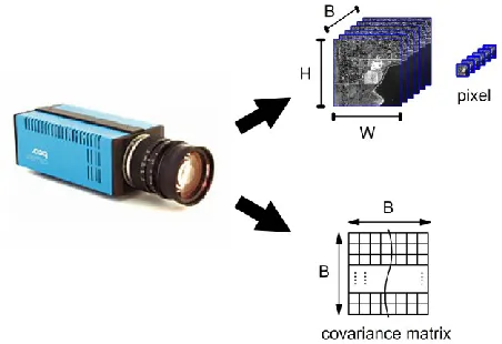
[image:1.612.325.551.518.673.2]Our proposal involves including dedicated signal processing within the HSI devices so their sequential acquisition of data (see Section 2.2) can be exploited for alternative covariance construction (Fig. 1), relieving memory requirements and allowing real time computation of the covariance matrix.
2.1. Conventional covariance matrix computation
Given a pixel vector xn[xn1,xn2,,xnB]T in a
hyper-cube of dimensions HWB, where B is the number of spectral bands, the procedure here consists of partitioning the 3-D hypercube into a 2-D data matrix namely
HW B HW
[p1,p2, ,p ]
P
, where the initial pixels
xnare subtracted the mean value HW HW
n1 n/
x
x , resulting
in pn[pn1,pn2,,pnB]T so the covariance matrix is ob-tained by the following multiplication, where the dividing term is omitted for simplicity.
B B T
PP
C . (1)
Even though this calculation is straightforward for mod-ern computers, this conventional procedure still has some drawbacks, as large dimensions of HSI hypercubes can lead to memory and computation problems, making implementa-tion in portable or embedded systems unfeasible. For that reason, we propose a simple approach for obtaining the covariance matrix ‘on the fly’ simultaneously with the ac-quisition process.
2.2. HSI acquisition procedures
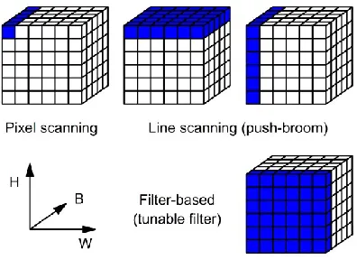
[image:2.612.316.556.237.348.2]The data capture present in current HSI devices and cameras can be divided into two groups: scanning and filter-based methods. On one hand, scanning techniques consist of a sequential procedure where the final image cube is obtained from partial spatial scenes, these may involve pixel scanning when individual pixels are acquired in every step, and line scanning (also known as push-broom technique) when spa-tial lines of pixels are captured to build the final image. Conversely filter-based methods collect the whole spatial scene at once but only for a particular spectral wavelength. Consequently, each spectral band is captured sequentially in every step. A schematic illustration of the different HSI acquisition techniques is shown in Fig. 2.
Fig. 2. HSI acquisition procedures [12].
2.3. ‘On the fly’ covariance matrix computation
Whichever acquisition technique is applied, it is clear that the procedure is sequential such that a series of small sub-spaces of the original data P
can be used to gradually
cal-culate the covariance matrix. This can result in faster im-plementations even up to real time.To this end, the partition by pixel pn (2), partition by row Ph(R) (3), partition by column Pw(C) (4), and partition by band Pb(B) (5) can be used as subspaces of data for con-structing the covariance matrix sequentially. These are de-fined as in Table 1.
Partition Subspace defined
Pixel pnB1 (2)
Row Ph(R)[ph,phH,,ph(W1)H]BW (3) Column ( )C
[
1 ( 1),
2 ( 1), ,
( 1)]
w
H w H w H H w B HP
p
p
p
(4)Band
W H HW
H
W H B
b
b b
b b
) ( )
(
) ( )
( ( 1) 1
1 ) (
p p
p p
P
[image:2.612.313.561.409.523.2](5)
Table 1. Proposed partitions and their defined subspace.
where the final covariance matrix is formed by the addi-tion of the partial covariance matrices shown in Table 2.
Partition Covariance matrix accumulation
Pixel
HW
n T n n pixel
1 )
( p p
C (6)
Row
H
h
T R h R h Row
1
) ( ) ( )
( P [P ]
C (7)
Column
W
w
T C w C w Col
1
) ( ) ( )
( P [P ]
C (8)
Band C(Band)(i,j)vec(Pb(Bi))[vec(Pb(B)j)]Ti,j[1,B] (9)
Table 2. Covariance matrix accumulation by the partitions.
2.4. Modification for real-time calculation
In cases where the covariance matrix computation is re-quired not only ‘on the fly’ within the HSI device but also in real-time, some modifications are required to include the mean subtraction procedure usually performed before multi-plication in (1).
[image:2.612.76.274.552.696.2]non-subtracted partitions xn, X(hR), and X(wC). As the mean subtraction procedure requires all pixel values within a spectral band, this leads to a correction for all our approach-es except the one using band partitions Pb(B).
Revisiting, the simple pixel partition problem, its corre-sponding multiplication can be expressed as
T n T n T n n T n n T n n x x x x x x M M x x p p
, (10)
where B B
n
M is a correction matrix calculated from the xn and the average pixel x, an expression simply de-rived from the product of subtracted values
) ( ) ( ) ( ) ( ) ( ) ( ) ( ) ( ) ( ) ( ) ( ) ( ) ( ) ( j i j i j i j i j j i i j i n n n n n n n n x x x x x x x x x x x x p p . (11)
Updating the covariance equation (6), now we have
CM x x C
HW n T n n pixel 1 )( , (12)
where the correction matrix CMBB, which is equivalent for the rest of partitions, is expressed as
HW n T n T n T HW n n 1 1 x x x x x x MCM . (13)
Simply developing this correction matrix, we have
HW n n HW n n HW n n n j i i j j i HW j i j i j i j i 1 1 1 ) ( ) ( ) ( ) ( ) ( ) ( )] ( ) ( ) ( ) ( ) ( ) ( [ ) , ( x x x x x x x x x x x x CM, (14)
where the second and third elements can be expressed as
) ( ) ( ) ( 1 ) ( ) ( ) ( ) ( 1 ) ( 1 1 j HW i j HW HW i i HW j i HW HW j HW n n HW n n x x x x x x x x
. (15)
Finally, CM is formulated as (16), which means it can be calculated in real time, at each iteration
HW n n HW nn i j
HW j i HW j i 1 1 ) ( ) ( 1 ) ( ) ( ) ,
( x x x x
CM . (16)
3. EXPERIMENTS AND RESULTS
A complete evaluation of the different approaches is per-formed in order to show a comparison between them and in relation to the conventional case. Initially, the HSI data sets employed in the experiments are introduced and described. Then, mathematical equivalency among the approaches is demonstrated. Finally, a comparison in terms of memory requirements, complexity and simulated timing demon-strates the benefits of our proposed approach.
3.1. HSI datasets for evaluations
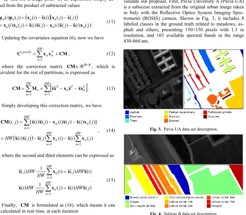
[image:3.612.65.562.235.670.2]Two data sets from different HSI sensors are employed to validate our proposal. First, Pavia University A (Pavia UA) is a subscene extracted from the original urban image taken in Italy with the Reflective Optics System Imaging Spec-trometer (ROSIS) camera. Shown in Fig. 3, it includes 8 labeled classes in the ground truth related to meadows, as-phalt and others, presenting 150×150 pixels with 1.3 m resolution, and 103 available spectral bands in the range 430-860 nm.
Fig. 3. Pavia UA data set description.
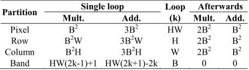
Fig. 4. Salinas B data set description.
[image:3.612.312.557.303.655.2]California, providing spatial resolution of 3.7 m in 204 valid spectral bands. It was acquired by the Airborne Visi-ble/InfraRed Imaging Spectrometer (AVIRIS) instrument. The ground truth here contains 9 classes corresponding to broccoli, lettuce, grapes and others.
3.2. Mathematical equivalencies
The fundamental assumption behind alternative implemen-tations of the covariance matrix is that the resulting final matrix obtained is exactly the same in all cases. Therefore, a simple example demonstrating mathematical equivalency is presented here.
In the conventional implementation in (1), the covari-ance matrix C is obtained from a large multiplication based on the original partition of data P. Accordingly, it is straightforward to express each element in matrix C as
) ( ) ( )
, (
1
j i j
i HW n
n n p p
C
.
(17)
Alternatively, for a simple pixel partition the subspaces multiplication leads to
n n
n B Bn
n n n
n T n n
B B B
B
) ( )
1 (
) ( 1 )
1 ( 1
p p p
p
p p p
p p p
. (18)
Simply by accumulating (18) for all pixels in the hyper-cube, the final covariance matrix is found as
B B HW
n
n n HW
n
n n
HW n
n n HW
n
n n pixel
B B B
B
1 1
1 1
) (
) ( )
1 (
) ( 1 )
1 ( 1
p p p
p
p p p
p
C
(19)
which provides the same values as the conventional case (17) in the BB elements of the matrix. The equivalency of the rest of partitions can be proved in a similar way.
This equivalency can be also demonstrated in practical terms. Actually, the implementation by the different parti-tions leads to negligible differences in the covariance matrix elements, clearly below 0.001%.
Additionally, the application of PCA by means of the different covariance matrices (Table 3) proves again the equivalency, as regardless of the partition employed to compute the covariance matrix in the PCA method, exactly the same classification results in land-cover analysis are achieved, in this case by the Support Vector Machine (SVM) classifier with a rate of 30% for training the model.
Partition used Pavia UA Salinas B
[image:4.612.317.556.329.397.2]Conventional 96.45 ± 0.27 94.50 ± 0.16 Row 96.45 ± 0.27 94.50 ± 0.16 Column 96.45 ± 0.27 94.50 ± 0.16 Pixel 96.45 ± 0.27 94.50 ± 0.16 Band 96.45 ± 0.27 94.50 ± 0.16
Table 3. Classification accuracy (%) using PCA (5 features).
3.3. Memory requirements
By using smaller partitions of data, which can be accessed during the sequential acquisition in HSI devices, the first clear advantage is the reduced size of the multiplying matri-ces for covariance calculation. The diverse sizes and contig-uous memory requirements for the different partitions are compared to the original case in Table 4.
Each partition sees its size reduced by a factor related to its dimensionality in the hypercube. Therefore, the pixel partition gives the highest reduction for the current data sets. Memory is expressed in kB, where data format considered is 8 bytes per value (double).
Partition Matrices size Pavia UA Salinas B
[image:4.612.68.299.444.522.2]Original B×HW 18540 36720 Pixel B×1 0.83 1.63 Row B×W 124 490 Column B×H 124 122 Band 1×HW 180 180
Table 4. Size of matrices and memory requirements (kB).
3.4. Number of multiplications and additions
The global number of multiplications and additions for all the cases is just the same, due to the equivalent implementa-tions. However, there is a small difference when the imple-mentation is performed in real time.
In the real time case, partitions require different com-plexity in each iteration (loop), with additional operations to be undertaken once the iteration process is completed, as can be seen in Table 5.
A trade-off between loop complexity and number of it-erations is easily recognizable when using different parti-tions. However, only the band partition is free of further calculations after the sequential acquisition. This is simply because the real-time correction is not necessary, as the average procedure is already included in the iterations.
Partition Single loop Loop (k) Afterwards
Mult. Add. Mult. Add.
Pixel B2 3B2 HW 2B2 B2
Row B2W 3B2W H 2B2 B2
Column B2H 3B2H W 2B2 B2
Band HW(2k-1)+1 HW(2k+1)-2k B 0 0
[image:4.612.314.557.619.688.2]3.5. Simulated timing comparison
Finally, to give an idea of the efficiency resulting from our proposal, a simulation of execution time required after ac-quisition in real time covariance computation is presented. These experiments are performed using MATLAB 8.0 on a PC with 3.1 GHz CPU and 8 GB Memory.
Fig. 5 shows the total execution time required just after the sequential acquisition process is finalised by the corre-sponding partition. Our approaches take advantage of the time gap between sequential acquisitions of partitions; therefore, this gap can be employed for real-time computa-tion, which includes partial covariance accumulation and related issues such as memory access and data transfer.
Once the acquisition process is completed (red line in Fig. 5), band partitions require no further operations, while the remaining row, column and pixel partitions still need a few milliseconds to complete the covariance calculation. Nevertheless, these times are very small in comparison to the timing needed if the original partition is selected, which clearly shows the efficiency involved by the ‘on the fly’ real time calculation.
Fig. 5. Simulated timing for different partitions.
4. CONCLUSIONS
The fast growth and remarkable development experienced by HSI technology in recent years has dramatically in-creased its use as it becomes a tool with enormous potential and a promising future. Due to the high dimensionality of the hypercubes, large volumes of data must be processed. Common preprocessing techniques such as PCA and others, require access to the covariance matrix. To this end, its efficient computation is of huge value in many HSI applica-tions.
However, covariance acquisition from high dimensional HSI data sets suffers from huge drawbacks, especially in portable and embedded systems, due to restricted capacities in terms of memory and computation power. For this reason,
we propose an ‘on the fly’ procedure, which makes the computation of the covariance matrix feasible in real time directly from HSI devices with embedded processing.
REFERENCES
[1] S. Sumriddetchkajorn, and Y. Intaravanne, “Hyperspectral imaging-based credit card verifier structure with adaptive learning”, Applied Optics vol. 47, no. 35, pp. 6594-6600, 2008.
[2] T. Kelman, J. Ren, and S. Marshall, “Effective classification of Chinese tea samples in hyperspectral imaging”, Artificial Intelligence Research, vol. 2, no. 4, pp. 87-96, 2013.
[3] X. Jia, B-C. Kuo, and M. M. Crawford, “Feature mining for hyperspectral image classification”, Proceedings of the IEEE, vol. 101, no. 3, pp. 676-697, March 2013.
[4] J. Zabalza, J. Ren, Z. Wang, S. Marshall, and J. Wang, “Sin-gular spectrum analysis for effective feature extraction in hy-perspectral imaging,” IEEE Geoscience and Remote Sensing Letters, vol. 11, no. 11, pp. 1886–1890, November 2014. [5] J. Zabalza, J. Ren, J. Zheng, J. Han, H. Zhao, S. Li, and S.
Marshall, “Novel two-dimensional singular spectrum analysis for effective feature extraction and data classification in hy-perspectral imaging,” IEEE Transactions on Geoscience and Remote Sensing, vol. 53, no. 8, pp. 4418–4433, August 2015. [6] I. Dopido, A. Villa, A. Plaza, and P. Gamba, “A comparative
assessment of several processing chains for hyperspectral im-age classification: What features to use?”, in Proc. WHISPERS, 2011.
[7] X. Jia and J. A. Richards, “Segmented principal components transformation for efficient hyperspectral remote-sensing im-age display and classification”, IEEE Trans. Geoscience and Remote Sensing, vol. 37, no. 1, pp. 538-542, January 1999. [8] J. Zabalza, J. Ren, M. Yang, Y. Zhang, J. Wang, S. Marshall,
and J. Han, “Novel Folded-PCA for improved feature extrac-tion and data reducextrac-tion with hyperspectral imaging and SAR in remote sensing”, ISPRS Journal of Photogrammetry and Remote Sensing, vol. 93, pp.112-122, July 2014.
[9] J. Ren, J. Zabalza, S. Marshall, and J. Zheng, “Effective fea-ture extraction and data reduction in remote sensing using hy-perspectral imaging [Applications Corner]”, IEEE Signal Processing Magazine, vol. 31, no. 4, pp. 149-154, July 2014. [10]R. Jošth, J. Antikainen, J. Havel, A. Herout, P. Zemčík, and
M. Hauta-Kasari, “Real-time PCA calculation for spectral im-aging (using SIMD and GP-GPU)”, Journal of Real-Time Im-age Processing, vol. 7, no. 2, pp. 95-103, April 2012. [11]M-Z. Wang, D-M. Wang, W-X. Xu, B-Y. Chen, and K. Guo,
“Parallel computing of covariance matrix and its application on hyperspectral data process”, in Proc.Geoscience and Re-mote Sensing Symposium (IGARSS), 2012.
[image:5.612.84.279.334.502.2]