Simulation of density measurements in plasma wakefields using photon acceleration

Simulation of density measurements in plasma wakefields using

photon acceleration

Muhammad Firmansyah Kasim,1 Naren Ratan,4 Luke Ceurvorst,4 James Sadler,4 Philip N. Burrows,1 Raoul Trines,2 James Holloway,3,*Matthew Wing,3

Robert Bingham,2 and Peter Norreys4,2 1

John Adams Institute, Denys Wilkinson Building, Keble Road, Oxford OX1 3RH, United Kingdom 2

STFC Rutherford Appleton Laboratory, Chilton, Didcot OX11 0QX, United Kingdom 3

Department of Physics and Astronomy, University College London, Gower Street, London WC1E 6BT, United Kingdom

4

Clarendon Laboratory, Department of Physics, University of Oxford, Parks Road, Oxford OX1 3PU, United Kingdom

(Received 13 June 2014; published 17 March 2015)

One obstacle in plasma accelerator development is the limitation of techniques to diagnose and measure plasma wakefield parameters. In this paper, we present a novel concept for the density measurement of a plasma wakefield using photon acceleration, supported by extensive particle in cell simulations of a laser pulse that copropagates with a wakefield. The technique can provide the perturbed electron density profile in the laser’s reference frame, averaged over the propagation length, to be accurate within 10%. We discuss the limitations that affect the measurement: small frequency changes, photon trapping, laser displacement, stimulated Raman scattering, and laser beam divergence. By considering these processes, one can determine the optimal parameters of the laser pulse and its propagation length. This new technique allows a characterization of the density perturbation within a plasma wakefield accelerator.

DOI:10.1103/PhysRevSTAB.18.032801 PACS numbers: 52.38.Kd, 52.65.Rr, 41.75.Jv, 42.30.Lr

I. INTRODUCTION

Plasma acceleration has been receiving interest recently since it can accelerate electrons up to GeV energy with a length much shorter than conventional accelerators[1–4]. In a plasma accelerator, a driver beam disturbs the plasma and generates wakefields. The driver can be a short laser pulse

[5], beat wave[6], electron beam[7], or proton beam[8]. Longitudinal electric fields generated in the plasma can reach tens or hundreds of GeV=m[9–11]. However, there are only a few techniques to measure and diagnose the perturbed density in the plasma. One of the earliest methods to diagnose the plasma wave is frequency domain inter-ferometry (FDI)[12]. FDI uses two short laser pulses and measures their phase difference caused by a different refractive index and density of plasma at certain positions. By using the FDI technique, one can only determine the density of plasma at certain single points. Therefore, to make a density profile, it needs many shots of short probe pulses at different positions.

Another technique which is a development of FDI is frequency domain holography (FDH) [12,13]. The FDH

technique needs one short reference pulse and one long probe pulse for measurement. However, to diagnose plasma wakefields with wavelength of the order ofμm, one needs a very short duration reference pulse (τ∼fs), which is much less than the wakefield wavelength. The other FDH technique uses two long duration chirped pulses [14,15]. By providing a wider frequency span of the chirped pulse, this technique could give more accurate results than the previous one that uses one short and one long pulse[12,13]. Another plasma imaging technique is the shadowgraph technique[16]. With this technique, the second derivative of the density with respect to the position is obtained. However, it is hard to extract quantitative data from the results of this technique because it needs small density perturbations to get precise results.

One possible technique to measure the density profile of plasma wakefields is to use photon acceleration first introduced by S. C. Wilkset al.[17]and further developed in Refs.[18–20]. In photon acceleration, a long probe pulse copropagates with the plasma wave and the change in frequency of the pulse is measured. The frequency change of the pulse is caused by the gradient of the plasma density profile. From this information, one can extract the density profile from the probe’s frequencies.

In this paper, the measurement of the wakefield density profile using the photon acceleration technique is simu-lated. In the simulation, we obtained two values of density profiles. The first is calculated from the probe’s frequency changes, which are now defined as the“measured”values *

John Adams Institute, Denys Wilkinson Building, Keble Road, Oxford OX1 3RH, United Kingdom.

in the rest of this paper. The second is obtained directly from the simulation, which are defined as the “actual” values. The measured values are then compared with the actual values in order to estimate the accuracy of the technique.

This paper is organized as follows. In Sec. II, we introduce a basic theory of photon acceleration and how it relates the plasma wakefield parameters with the probe’s frequency changes. The simulation parameters and the data processing technique are described in Sec. III. In the next section, we discuss the results and limitations of the photon acceleration technique. Last, in Sec.Vwe give a conclusion of this paper.

II. PHOTON ACCELERATION

When a photon moves in a medium which has a refractive index varying with time, the photon will undergo a change in frequency. Wakefields propagate along the plasma and have a different refractive index at every position. Thus, if a laser copropagates with the wakefield, the laser frequency will change after some propagation length.

Using photon ray theory by Mendonça [21], the fre-quency change of a laser copropagating with a plasma wakefield can be obtained as:

Δω ω0 ≈ −

ω2 p

2ω2 0

1 n₀

Z

∂n

∂ζds; ð1Þ

whereΔωdenotes the frequency change of the laser,ω₀the central frequency of the laser, nandn₀ are the perturbed and initial plasma density, respectively, ω_p≈k_pc the plasma frequency,k_pthe plasma wave number,cthe speed of light in vacuum,sthe propagation length of the laser, and ζ¼z−ctdenotes the position relative to the laser’s frame of reference with z andt as position and time in the lab frame, respectively. This expression is also discussed by Diaset al.[18].

In order to get the density profile, one needs a long laser pulse that samples several plasma wavelengths. By doing so, one can obtain the average density over the propagation length for every position in the laser’s frame of reference. In a real experiment, it is possible to measure the frequency change of a laser at every longitudinal position using frequency resolved optical gating (FROG) diagnos-tic. Schreiber et al. [22] have used the second harmonic generation (SHG) FROG to get the complete temporal characterisation of a laser pulse: amplitude and phase.

III. METHODS

A. Simulation parameters

Simulations were performed using OSIRIS 1D relativ-istic code [23] on the SCARF-LEXICON machine at STFC Rutherford Appleton Laboratory. OSIRIS uses a

particle in cell (PIC) [24] algorithm to solve differential equations to determine electromagnetic fields and the phase space of particles. Particles in PIC codes are modeled using the super-particle model. A super-particle is a computa-tional particle which represents many real particles. Electromagnetic fields in PIC codes are determined from the positions and momenta of the particles and thus will act on the particles, changing those parameters.

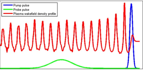
In this paper, a case for the use of a diagnostic based on photon acceleration is presented. In the baseline setup, we send a short pump pulse with wavelength of 800 nm and with duration of 39 fs to a plasma with density of 2×1018 cm−3. The intensity of the pump pulse is 4.7×1018 W=cm2, which gives a normalized potential ofa₀¼1.5, to drive a nonlinear wakefield. In the plasma, the pump pulse generates a plasma wakefield which will be diagnosed using a probe pulse. The probe pulse is sent behind the pump pulse with the same wavelength but with a longer duration, 300 fs. The intensity of the probe pulse is much lower than the pump pulse, 2.1×1014 W=cm2, which corresponds toa₀¼0.01. These pulses propagates through the plasma for a distance of about 7 mm. The numbers are chosen to have the same order of magnitude with common parameters of laser plasma wakefield accel-erator experiments[1–4]. A simple sketch of this setup is shown in Fig. 1.

As the amplitude of plasma wakefield is approximately proportional to a2₀ of a laser pulse [9], the wakefield generated by the probe is 5 orders of magnitude smaller than the wakefield generated by the pump pulse. So we can safely assume that the wakefield produced by the pump pulse is not disturbed by the probe pulse.

In this paper, the probe pulse is an unchirped, transform-limited pulse. The cases of using chirped probe pulse will be the subject of future studies.

B. Obtaining the local frequency

The photon acceleration technique relies on local fre-quency profile measurement of the probe pulse. In the wave model, local frequency is defined as the derivative of the phase with respect to time. Moreover, in the photon model,

it is defined as the average frequency of photons at that point. In this section, we describe how to get the local frequency in simulations and in a real experiment.

The simulation produces the actual density profile and the transverse electric field of the pump and probe pulse. We apply a transformation to the probe pulse’s electric field to get its Wigner distribution[25]to represent the wave energy distribution in phase space or in time-frequency space. The Wigner distribution of a signal is represented by:

WEðζ; kÞ ¼

Z _∞

−∞Eðζþζ

0_{=2ÞEðζ−ζ}0_=2Þe−ikζ0

dζ0 ð2Þ

where EðζÞ is electric field of the signal at position ζ relative to the laser’s frame of reference andk¼2πf=cis the wave number of the laser. Because there are two terms of the signal multiplied together, there are cross terms in the distribution [26].

By taking the average and weighted average of the Wigner distribution, one can get local intensity and local frequency of the probe pulse in air, as shown in the equations below,

jEðζÞj2_¼ 1

2π

Z _∞

−∞WEðζ; kÞdkfðζÞ ¼ c

2π 1 jEðζÞj2

Z _∞

−∞kWEðζ; kÞdk: ð3Þ

From the equations above, it appears thatΔf=f∝ΔE=jEj. Thus, if there is noise in E in simulations, the measure-ments offare less accurate at points with lower intensities. To get the local frequency in a real experiment, one can employ frequency resolved optical gating (FROG) diag-nostic. The diagnostic takes place in air, outside of the plasma and its containment vessel. The dispersion relation in air is approximately ω≈kc=n with refractive index n¼1.0003≈1. This makes the temporal profile evolution of the probe pulse negligible after it leaves the plasma because the dispersion relation of air is close to vacuum. The intensity of the probe pulse is also low enough to keep the air from ionization.

One type of FROG is the second harmonic generation (SHG) FROG which was used in Schreiber’s experiment

[22]. When a laser pulse enters the SHG FROG, the diagnostic then produces a trace as below,

ISHG

FROGðk;ξÞ ¼

Z_−∞∞EðζÞEðζ−ξÞe−ikζ_dζ2_{: ð4Þ}

The diagnostic uses a Fresnel biprism to split the pulse into two pulses with varied delay to each other, a thick SHG crystal to combine these two pulses and splits the combined pulse into its frequency component. These components make it possible to get the trace in a single shot. From the trace, the temporal intensity profile, jEðζÞj2, and phase

profile,ϕðζÞ, of the pulse can be retrieved using a retrieval algorithm[27–29].

The retrieval algorithm first sets an initial guess ofEðζÞ. The algorithm then iteratively updates the guess to match the FROG trace from the experiment. After it reaches a convergence, the algorithm then shows the last guess of EðζÞ as the measured electric field, including its intensity and phase. From the measured phase profile, the local frequency in air can be obtained by

fðζÞ ¼ c 2π

∂ϕðζÞ

∂ζ : ð5Þ

The retrieval algorithm can produce accurate results of the intensity and phase profile. It has been reported several times that the root mean square (rms) error from the retrieval algorithm is less than 0.5% for SHG FROG

[27–29].

Although the rms error reaches below 0.5%, the phase profile cannot be determined accurately where the probe’s intensity is too small compared to its peak intensity. The frequency change where the probe’s intensity is very small does not induce a significant change to the FROG trace. Therefore, the retrieval algorithm cannot determine accurately the phase at that point.

C. Integration filter

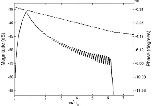
Equation(1)shows that one can obtain the average value of ∂n=∂ζ if the frequency change is measured. Thus, in order to get the electron density distribution, the frequency-change term needs to be integrated once with respect to position in the laser’s frame of reference,ζ. However, if the integration is done by getting the cumulative sum of ∂n=∂ζ, a small DC offset could cause the result being tilted. In order to suppress the DC offset error, one can apply a custom digital filter to do the integration. Figure2shows

the amplitude and phase response of an example filter. For a normal integration filter, the amplitude response at low frequency is very high. Thus in the filter, the amplitude response at the low frequency is suppressed to avoid the result being tilted as in Fig.3. The high frequency terms in the filter is also removed to avoid unwanted noise in the signal. The oscillating amplitude response at high fre-quency is due to imperfect filter (i.e., limited number of coefficients in the filter). The filter design does not need a prioriknowledge of the density profile. It is flexible as long as it suppress low and high frequency terms and has similar form with a normal integration filter forω=ω_p≥1.

IV. RESULTS AND DISCUSSION

A. Simulation of measurement results

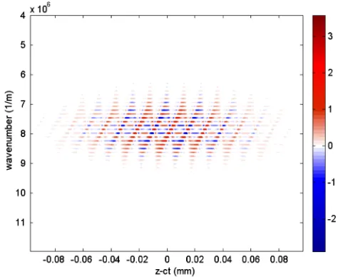
From the simulation results, we obtain the electric field of the probe pulse. Applying Eq. (2) produces the Wigner distribution of the signal in phase space. One example of the Wigner distribution of a signal is shown in Fig.4. In the distribution, the photon acceleration effect is observed. The frequency at some positions increases and decreases. Inserting this frequency profile into Eq.(1), one can obtain the measured density profile of the wakefield. The measured values can be compared with the actual density profile of the wakefield which is obtained directly from the simulation.

From the Wigner distribution of the electric field, one can get the local frequency for every position in the laser’s reference frame using Eq.(3). According to the equation, the accuracy of the measurement would be good if the intensity at that point is not very small or not too far from the probe’s centre. Because of that, we did the measure-ments only at positions where the intensity is more than 0.5% of the maximum intensity. At the other positions, we take the frequency change as zero. The lower one chooses the threshold value, the wider measurement result becomes, but the inaccuracy also increases. We chose the value of

0.5% to get wide measurement results while still main-taining the accuracy.

Figure 5 shows the comparison between the measured electron density and the actual density over the distance. At z−ct <0.1mm, there is some simulation noise in the actual values. Over propagation length less than 6 mm, the measurement agrees well with the actual average value. However, if the laser pulse propagates too far, the meas-urement fails to match with the actual value. This is because of the photon trapping effect, which we will explain in Sec.IV B 2.

In order to determine the accuracy of the measurement, we provide the normalized root mean square error (NRMSE) between measurement and actual values. The NRMSE is defined by

NRMSE¼ RMSE

maxðn_aÞ−minðn_aÞ

RMSE¼

ffiffiffiffiffiffiffiffiffiffiffiffiffiffiffiffiffiffiffiffiffiffiffiffiffiffiffiffiffiffiffiffiffiffiffiffiffiffiffiffiffiffiffiffiffiffiffiffiffiffiffiffiffiffiffiffiffiffiffiffiffi

1 ζf−ζ0

Z _ζ

f

ζ0

½n_mðζÞ−n_aðζÞ2_dζ s

ð6Þ

whereζ₀andζfdenote the lower and upper range in position

where the NRMSE is calculated,nmðζÞ and naðζÞ

respec-tively denote the measured and the actual values as function of position in the laser’s reference frame,ζ. The choice of range ζ₀ and ζ_f depends on the probe pulse’s duration. Longer ranges can be chosen for longer probe pulse durations. Note that before calculating the NRMSE values, we removed the noise at z−ct <0.1mm from actual density values by applying a low pass filter.

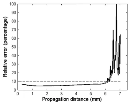
The NRMSE of the measurement is shown in Fig. 6

for several propagation lengths. As shown in the graph, the measurement achieves less than 10% NRMSE over the FIG. 3. Comparison of integration results using designed filter

(solid line) and cumulative sum (dashed line).

propagation length of less than 6 mm. After the probe pulse propagates 6 mm, the error increases and becomes unstable. This is where the photon trapping effect occurs.

Although the deviation seems larger at small propagation lengths (from Fig. 5), the error is smaller at small propa-gation length according to Fig.6. This is mostly caused by noise which is suppressed using a low pass filter before calculating the NRMSE values.

B. Measurement constraints

In doing measurements using the photon acceleration technique, there are several constraints and limitations that one needs to take into account. The constraints and limitations can spoil the measurement, but they can be minimized by providing the correct parameters.

1. Small frequency change

The first limitation is when the frequency change is not observable. The frequency change in photon acceleration in some cases is very small and thus very hard to measure precisely. We can take the AWAKE experiment[30]as an

example. In the AWAKE experiment, the plasma density is n₀¼7×1014 cm−3, laser wavelength is 800 nm, propa-gation length is 10 m and the relative density perturbation is aboutΔn=n₀∼0.1–0.5. Based on Eq. (1), the frequency change is about∼0.3%of the initial frequency. Thus one needs diagnostics with frequency precision up to∼0.003% around 800 nm to make a good measurement with 1% precision of the frequency shift. With the technology of FROG that can measure the frequency change up to ∼0.0003%, this technique can be applied to a plasma with density as low as∼1×1014 cm−3, using the same propa-gation distance and density perturbation with the AWAKE experiment. The number can be lower for longer plasma column or with more precision and accurate diagnostic tools. Moreover, a short pulse can have a broad frequency spectrum. If the pulse is too short and the frequency change is too small, it would be also too hard to observe the frequency change. In order to make the measurement easier, the laser’s frequency change should be greater than bandwidth of the pulse orΔω>ω_bw. By considering the Gabor limit [31], τpulseðωbw=2πÞ≥1=2, and Eq. (1), the

minimum duration of the probe pulse should be

τpulse >

2πω0n0

ω2 ps

∂n ∂ζ

₋₁

; ð7Þ

where ω₀ is the central frequency of the pulse, n₀ is the density of the plasma, ω_p is frequency of the plasma wakefield,sis the propagation length, and∂n=∂ζis partial derivative of electron density to the position in the laser’s frame of reference.

In this case, the minimum pulse duration is about 3 fs, much smaller than the plasma wavelength which is around 80 fs. Therefore this limitation is not significant in this case. However, this limitation should be considered when doing measurement at low density plasma.

2. Photon trapping

In photon acceleration, the frequency of some photons increase and some decrease. Based on the plasma dispersion relation, ω2¼ω2pþk2c2 (where k is wave number of

photons), the photons whose frequencies increase will acquire higher group velocity and the others will acquire lower group velocity. The difference of this group velocity causes some photons to be gathered in the troughs and be away from the peaks of the wakefield. This mechanism is called photon trapping[21], which is one form of modu-lation instabilities[32–34].

Photon trapping could affect measurements with photon acceleration technique. As the intensity of the laser at some points approaches zero, the error in obtaining the frequency will be very high and could cause high inaccuracy.

The photon trapping mechanism starts when the laser enters the plasma. However, this effect is negligible at the beginning and would become significant after propagating some distance. One can estimate the propagation scale length in which the photon trapping would be significant. The propagation scale length is proportional to

s_trap∝λpðω0=ωpÞ2ðδn=n0Þ−0.5; ð8Þ

whereλ_pis the plasma wavelength andδn=n₀is the relative perturbation of the wakefield.

For the laser and plasma parameters considered here, the value of the right-hand side of Eq.(8)is about∼30mm. From Fig. 6, the photon trapping effect is observed at 6 mm. Therefore, the photon trapping effect should be considered after propagated about 20% of the right-hand side value of Eq. (8). By considering this propagation length limit, the photon acceleration measurement can be applied to a plasma with density up to∼4×1018 cm−3in a 2 mm gas jet. The number can be higher for higher probe’s frequency or a narrower gas jet.

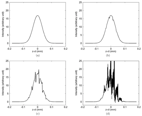
One way to determine if the photon trapping should be taken into account is by looking at the intensity distribution of the laser obtained by Eq.(3). Figure7shows the probe laser’s intensity distribution at several propagation lengths. As shown in the figures, the laser intensity gets modulated as it travels along the plasma. And at some distance, the laser intensity at some points go to zero and intensity at some points become very high as shown on Fig.7d. This shows that the photon trapping has occurred.

3. Laser displacement

Up to this point, we assumed that the laser is always moving along with the wakefield. However, this may not be true for all cases. If the group velocity of the probe pulse is not the same as the phase velocity of the wakefield, the laser could be displaced with respect to the wakefield. This could happen if the experiment uses a particle beam to drive the wakefield[30]. In other cases, one might employ different frequencies between the pump and the probe pulses to more easily distinguish between them[14]. There are also cases where the pump pulse is depleted, so it propagates slightly less than its group velocity [35]. In those cases, the laser displacement should be considered because it changes the measurement values.

To show the effect of laser displacement, another simu-lation is performed with the same conditions but with a probe wavelength of 1600 nm. Figure 8shows the measurement result using this probe compared with the actual average density after it travels 1.4 mm in the plasma wakefield. As shown in the figure, the measurement result is shifted backward by 1.6μm and slightly smaller than the actual value. This shift is caused by the difference of group velocity of the probe pulse and phase velocity of the wakefield.

Using Eq. (1) and by considering that the pulse is moving relative to the wakefield, a total shift of the measurement is obtained as,

Δs≈sðv_g−v_pÞ=2v_p; ð9Þ

wherevgandvpare group velocity of the laser probe pulse

and phase velocity of the plasma, respectively, andsis the propagation length. Equation (9) also assumes that the FIG. 6. Normalized root mean square error (NRMSE) between

wakefield amplitude and wavelength is constant and not changing over time. For the case with probe wavelength of 1600 nm, Eq. (9)gives Δs¼−1.2μm with s¼1.4mm, while the simulation result gives −1.6μm.

Besides the horizontal shifting, the laser displacement effect also caused the measurement values to be scaled down slightly. By doing the same derivation with Eq.(9), one can get the decrement of the measured values because of laser displacement as below,

Δn n−n₀≈ −

1

24k2ps2ðvg−vpÞ2=c2: ð10Þ

Thus, if the laser propagates for long distance, the correc-tion above should be taken into account to improve the measurement accuracy.

4. Stimulated Raman scattering

If a laser pulse propagates in plasma for quite a long distance, the oscillation in plasma can lead to the generation

of electrons and ions waves in various directions, e.g., stimulated Raman scattering (SRS) and stimulated Brillouin scattering (SBS), etc. In this model, SBS growth is negligible since the laser intensity is very small. For SRS, the scattered wave that can spoil the measurement is the forward-scattered wave.

Along the probe pulse propagation in the plasma, the scattered wave grows exponentially and propagates together with the probe pulse. In order to maintain a good measurement, the amount of exponentiation,κ, should not be too large. According to Antonsen and Mora[36], the amount of exponentiation of a pulse with durationτ is

κ¼ ða2

0kpω2psτ=2ω0Þ1=2 ð11Þ

where a₀ is normalized intensity of the laser and s is the propagation length. To estimate the maximum laser intensity, the amount of exponentiation is set to unity and solved fora₀,

a₀≲ð2ω0=kpω2psτÞ1=2: ð12Þ

Intensities slightly larger than(12)are still permitted as long as they are not much larger. For the simulation case in this paper,κ≈0.25for propagation length of 6 mm. The value gives the grow factor ofeκ≈1.3which indicates that the scattered wave does not grow significantly.

5. Laser beam divergence

In the simulations presented in this paper, we assume that the electromagnetic wave is a plane wave propagating in thezdirection. However, for a finite transverse size of the laser pulse, its Rayleigh length [37] must be taken into consideration.

In order to use this diagnostic technique, one needs the probe pulse to be collimated along the propagation length. It is assumed that the laser is collimated when the beam’s waist size isw < w₀pffiffiffi2withw₀as its minimum waist size. The condition implies that the total propagation length must be shorter than twice of its Rayleigh length. To achieve this condition, one needs the beam’s waist size of

w₀>ðsc=ω0Þ1=2: ð13Þ

If the beam waist is larger than the transverse size of the plasma wakefield, one can put an optical aperture in front of the FROG to sample only that part of the probe that diagnoses the plasma wakefield. If the laser pulse is tight focused at a particular position, it will sample the plasma wave only at that point. This will be the subject of a future study.

V. CONCLUSIONS

Results from our simulation show that the measurement of a density profile in a plasma wakefield can be performed using photon acceleration. The measurement is done by sending a long laser probe pulse behind the short pump

pulse which generates the wakefield. From our simulation results, the measurement values achieve a normalized root mean square error of less than 10%, although the exact value needs to be determined for a given set of experimental parameters.

There are also constraints to be considered before doing a photon acceleration measurement. Those are small fre-quency changes, photon trapping effects, laser displacement, stimulated Raman scattering, and laser beam divergence. If the propagation length is too small, then the frequency change could be undetectable. However, if the propagation length is too far, the photon trapping effect and the stimulated Raman scattering could spoil the measurement result. Also, if the probe’s group velocity is not same as the phase velocity of the wakefield, the inaccuracy of the measurement could also increase. By considering these effects, one can determine the optimal parameters of the probe and propagation length for a given set of experimental parameters. This technique can be applied on laser wakefield experiments with plasma density from ∼1×1014cm−3 to ∼4×1018 cm−3with reasonable experimental parameters.

ACKNOWLEDGMENTS

The authors would like to acknowledge the support from Engineering and Physical Sciences Research Council, the Central Laser Facility, and the Computer Science Department at the Rutherford Appleton Laboratory for the use of SCARF-LEXICON computer cluster. We also wish to thank the OSIRIS consortium for the use of OSIRIS and also to the Science and Technology Facilities Council for its support to AWAKE-UK. One of the authors (M. F. Kasim) would like to thank Indonesian Endowment Fund for Education for its support. M. Wing acknowledges the support of DESY, Hamburg and the Alexander von Humboldt Foundation. The work is part of EuCARD-2, partly funded by the European Commission, GA 312453.

[1] S. P. D. Mangles, C. D. Murphy, Z. Najmudin, A. G. R. Thomas, J. L. Collier, A. E. Dangor, E. J. Divall, P. S. Foster, J. G. Gallacher, C. J. Hooker et al., Nature

(London)431, 535 (2004).

[2] C. G. R. Geddes, Cs. Toth, J. van Tilborg, E. Esarey, C. B. Schroeder, D. Bruhwiler, C. Nieter, J. Cary, and W. P. Leemans,Nature (London)431, 538 (2004).

[3] J. Faure, Y. Glinec, A. Pukhov, S. Kiselev, S. Gordienko, E. Lefebvre, J.-P. Rousseau, F. Burgy, and V. Malka,Nature

(London)431, 541 (2004).

[4] W. P. Leemans, B. Nagler, A. J. Gonsalves, Cs. Tóth, K. Nakamura, C. G. R. Geddes, E. Esarey, C. B. Schroeder, and S. M. Hooker,Nat. Phys.2, 696 (2006).

[5] T. Tajima and J. M. Dawson, Phys. Rev. Lett. 43, 267

(1979).

FIG. 8. Measurement result of longitudinal average electric field with probe wavelength of 1600 nm after traveling 1.4 mm. The measurement result (dashed line) is shifted backward by

[6] C. Joshi, W. B. Mori, T. Katsouleas, J. M. Dawson, J. M. Kindel, and D. W. Forslund, Nature (London) 311, 525

(1984).

[7] J. B. Rosenzweig, D. B. Cline, B. Cole, H. Figueroa, W. Gai, R. Konecny, J. Norem, P. Schoessow, and J. Simpson,Phys. Rev. Lett.61, 98 (1988).

[8] A. Caldwell, K. Lotov, A. Pukhov, and F. Simon, Nat.

Phys.5, 363 (2009).

[9] E. Esarey, C. B. Schroeder, and W. P. Leemans,Rev. Mod.

Phys.81, 1229 (2009).

[10] D. Gordon, K. C. Tzeng, C. E. Clayton, A. E. Dangor, V. Malka, K. A. Marsh, A. Modena, W. B. Mori, P. Muggli, Z. Najmudinet al.,Phys. Rev. Lett.80, 2133 (1998). [11] V. Malka, S. Fritzler, E. Lefebvre, M.-M. Aleonard,

F. Burgy, J.-P. Chambaret, J.-F. Chemin, K. Krushelnick, G. Malka, S. P. D. Mangles et al., Science 298, 1596

(2002).

[12] C. W. Siders, S. P. Le Blanc, A. Babine, A. Stepanov, A. Sergeev, T. Tajima, and M. C. Downer, IEEE Trans.

Plasma Sci.24, 301 (1996).

[13] S. P. Le Blanc, E. W. Gaul, N. H. Matlis, A. Rundquist, and M. C. Downer,Opt. Lett.25, 764 (2000).

[14] N. H. Matlis, S. Reed, S. S. Bulanov, V. Chvykov, G. Kalintchenko, T. Matsuoka, P. Rousseau, V. Yanovsky, A. Maximchuk, S. Kalmykov et al., Nat. Phys. 2, 749

(2006).

[15] A. Maksimchuk, S. Reed, S. S. Bulanov, V. Chvykov, G. Kalintchenko, T. Matsuoka, C. McGuffey, G. Mourou, N. Naumova, J. Neeset al.,Phys. Plasmas15, 056703 (2008). [16] A. Sävert, S. P. D. Mangles, M. Schnell, J. M. Cole, M. Nicolai, M. Reuter, M. B. Schwab, M. Möller, K. Poder, O. Jäckelet al.,arXiv:1402.3052.

[17] S. C. Wilks, J. M. Dawson, W. B. Mori, T. Katsouleas, and M. E. Jones,Phys. Rev. Lett.62, 2600 (1989).

[18] J. M. Dias, L. Oliveira e Silva, and J. T. Mendonça,Phys.

Rev. ST Accel. Beams1, 031301 (1998).

[19] C. D. Murphy, R. Trines, J. Vieira, A. J. W. Reitsma, R. Bingham, J. L. Collier, E. J. Divall, P. S. Foster, C. J. Hooker, A. J. Langleyet al.,Phys. Plasmas 13, 033108

(2006).

[20] R. M. G. M. Trines, C. D. Murphy, K. L. Lancaster, O. Chekhlov, P. A. Norreys, R. Bingham, J. T. Mendonça,

L. O. Silva, S. P. D. Mangles, C. Kamperidiset al.,Plasma

Phys. Controlled Fusion51, 024008 (2009).

[21] J. T. Mendonça, Theory of Photon Acceleration (CRC Press, Bristol, 2001).

[22] J. Schreiber, C. Bellei, S. P. D. Mangles, C. Kamperidis, S. Kneip, S. R. Nagel, C. A. J. Palmer, P. P. Rajeev, M. J. V. Streeter, and Z. Najmudin, Phys. Rev. Lett.105, 235003

(2010).

[23] R. A. Fonseca, L. O. Silva, F. S. Tsung, V. K. Decyk, W. Lu, C. Ren, W. B. Mori, S. Deng, S. Lee, T. Katsouleas et al.,Lecture Notes in Computer ScienceVol. 2329, III-342 (Springer, Heidelberg, 2002).

[24] C. K. Birdsall and A. B. Langdon, Plasma Physics via Computer Simulation(CRC Press, New York, 2004). [25] E. Wigner,Phys. Rev. 40, 749 (1932).

[26] P. Flandrin, Time-Frequency/Time-Scale Analysis (Academic Press, New York, 1999).

[27] K. W. DeLong, R. Trebino, J. Hunter, and W. E. White,

J. Opt. Soc. Am. B11, 2206 (1994).

[28] D. J. Kane, G. Rodriguez, A. J. Taylor, and T. S. Clement,

J. Opt. Soc. Am. B14, 935 (1997).

[29] D. J. Kane,IEEE J. Sel. Top. Quantum Electron. 4, 278

(1998).

[30] R. Assmann et al. (AWAKE Collaboration), Report No. CERN-SPSC-2013-013, http://cds.cern.ch/record/

1537318;arXiv:1401.4823.

[31] D. Gabor,Journal of the Institution of Electrical

Engineers-Part III: Radio and Communication Engineering93, 429

(1946).

[32] F. F. Chen,Introduction to Plasma Physics and Controlled Fusion, Vol. 1 (Springer, New York, 2006).

[33] K. Nishikawa, Advances in Plasma Physics, edited by A. Simon and W. B. Thomson (Wiley, New York, 1976), Vol. 6.

[34] R. Bingham and C. N. Lashmore-Davies, Plasma Phys.

Controlled Nucl. Fusion Res.21, 433 (1979).

[35] W. Lu, M. Tzoufras, C. Joshi, F. S. Tsung, W. B. Mori, J. Vieira, R. A. Fonseca, and L. O. Silva, Phys. Rev. ST

Accel. Beams10, 061301 (2007).

[36] T. M. Antonsen, Jr. and P. Mora,Phys. Fluids B 5, 1440

(1993).