VALIDATING WIND FIELD MODELS FOR POWER SYSTEM
IMPACT STUDIES
C. Plumley, D. Hill, D. McMillan, K. Bell, D. Infield
University of Strathclyde, Glasgow, UK E-mail: [email protected]
Keywords: wind resource; power system impact
Abstract
To integrate wind power into the electrical power system studies need to be made of its impact. Wind plants are stochastic in nature and this makes them differ from traditional plants. One method to model the stochastic nature of wind plants is to create a wind field model and simulate wind data that can then be used to determine power outputs. There are a large number of models available, however often these models are not adequately validated. This paper proposes a number of criteria that all wind field models should be validated against and the methods that can be used to do this.
1 Introduction
The twin fears of Climate Change and Peak Oil have prompted many countries to look at alternative energy sources, such as renewable electricity generation. One of the most commercially viable renewable technologies is wind energy, which has the potential to supply a large proportion of electricity demand worldwide. However, as wind penetration in power systems increases important decisions need to be made regarding investment in energy infrastructure, both to minimise curtailment of wind and ensure overall reliability of supply of electricity [6].
The stochastic nature of wind means power output from wind farms fluctuate on an hour to hour and day to day basis. This makes it difficult to predict power flows in a system using traditional techniques. By having a model that can predict the likely power output of wind farms a probability based model of power flows in the network can be produced. Reliability studies require long data sets, as the occurrence of rare events that are critical to the power system need to be captured. As data regarding wind farm outputs is currently limited, these models usually employ wind speed data to derive the power output of current and potential wind farms.
Although historical wind speed data is preferable to synthesised data, it is not always of sufficient quantity and quality. A model that can simulate data can overcome these problems [7]. Synthesised data can be used to fill previously missing data points, or replace erroneous data points, and can also be applied to different time periods or even to locations
where data has not previously been recorded giving a better representation of wind speeds across countries.
To make important decisions utilising such models, the models need to be rigorously validated and shown to accurately represent the wind field. Previous analyses have looked at various aspects, for example the distribution of wind speeds, the variability of the wind on an hour-to-hour basis and the duration and period of calms [12]. However, so far there has been a failure to validate models as regards to the effect of spatial and temporal correlation between regions, and the diurnal and seasonal trends in wind speeds that are important to match generation with demand.
In this paper a rigorous validation process is described that ensures all these characteristics are taken into account. This means where models are shown to be deficient, improvements can be made, and where limitations remain they are at least understood, thus permitting transmission system operators to make informed decisions about where to invest their capital and reinforce the network.
2 Literature review
Power system impact studies that take into account the integration of wind require models to simulate the variable nature of the wind plants. This can be done by either directly modelling the power outputs or by modelling the wind and then converting to electrical output using a suitable power curve. Due to the accessibility of wind data compared to wind farm power data, the later method is discussed in this paper as the preferred approach.
There are many types of wind field model being considered for use in power system impact studies; a comprehensive literature review of wind speed and wind power models is provided in [7].
effects required of long term simulations for power system planning [4,7].
Numerical weather predictions that model the physics of the weather system have also been used [2]. Although more detailed than statistical models, the added complexity has been considered inappropriate for power system impact studies [8].
Wind field models have tended to be validated by comparing the auto-correlation, probability density functions of the annual wind speed distributions and sometimes variability of the wind [8,9]. The Root Mean Square error (RMSe) in forecast predictions is also a common metric. The frequency and duration of calms has also been mentioned by a minority of authors [10,11,12]. These approaches are combined in this paper.
3 Wind system impact characteristics
Certain characteristics of the wind are of particular importance to assess the impact that increased wind penetration will have on the power system. The obvious difference between conventional and wind generation is the uncontrollable intermittency of the wind.
At times of low wind, areas that rely on wind power may have to import electricity from elsewhere, whereas at times of high wind regions with high wind penetration may be net exporters of electricity. A balance needs to be found that avoids excessive curtailment of wind while taking into account the costs associated with reinforcing the grid, all while maintaining reliability. This is looked at in [11]. A more developed approach will need to take into account which regions have a large amount of wind generation, and the variation of wind speeds between regions.
The duration of low wind periods is also important, as this effects the amount of storage required to balance out the grids energy requirements. Short term calms on the order of hours may be compensated for by pumped storage whereas longer periods will require reserve plants to be brought online. The choice of this support generation will be partly based on the characteristics of these calms, but will also depend on the variability of the wind.
During periods of high wind penetration, the variability of the wind will require increased levels of spinning reserve, both to cope with short term fluctuations and likely changes in wind speed. On time-scales of about 4 hours the variability is of particular importance, as this is the time required to start up a Combined Cycle Gas Turbine (CCGT) plant [12]. If a model can accurately predict the wind speed on the short term (i.e. 1-24 hours in advance) it would also be a useful tool in system operation, as well as system planning.
At timescales of 1 to 5 hours look ahead, wind farm owners are often required to give rolling forecasts, as a result it is important to have an economic, efficient and reliable method
for producing these forecasts. In other countries, the system operator takes on this responsibility; however it is equally important, for the same reason, that they have an accurate prediction model. Longer range forecasts of 5 plus hours will allow the wind farm operators to plan and carry out maintenance efficiently, rather than basing maintenance strategy on seasonal trends [5].
4 Validation procedure
Validation is, as described in the Literature review, often done using measures such as the RMSe forecast prediction, comparison of the auto-correlation function or through pdfs of the annual wind speed distribution. Although these cover some of the criteria mentioned above, certain aspects are lacking, and it is rare that a full validation process is considered. In this paper a clear description of a number of validation tools is given. It is hoped these will aid in the proper validation of future wind field models and highlight the deficiencies that likely exist in a number of the current models. The methods proposed are designed to be clear to the user what the impact of the model not aligning to real data has, rather than abstract statistical metrics which are harder to interpret, such as looking at the auto-correlation function.
For illustrative purposes the VAR model developed by the authors is used to demonstrate the various validation techniques proposed [7]. The time steps are of one hour, however more concentrated data may also be used. The comparisons are also given in a “per year” scale, so that simulations can be run of various lengths and still be compared. Error bars are of 2ʍ, showing a 95% confidence level.
4.1 Annual wind speed distribution
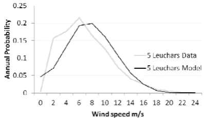
[image:2.595.309.508.621.736.2]The probability distribution of hourly wind speeds over the course of a year is important in energy calculations to determine the total energy a wind plant will produce. It also shows whether the model is properly simulating both low and high wind speed events. For example in Figure 1 low wind speeds appear to be under-represented, whereas near and above rated wind speeds are over-represented. This will result in an over-estimation of the total energy the wind plant will produce during a year and in power flow simulations this will lead to incorrect predictions about the proportion of times with high and low wind penetrations.
A measure to help quantify how well the model matches with the data is a simple RMSe calculation of the probability distributions. To do this the difference between the model-generated pdf (Pmodel,b) and the real data pdf (Pdata,b) at a series of wind speed bins is taken (see Equation (1)), where B is the total number of wind speed data bins and b is the individual wind speed bin).
¦
B bb data b
el
P
P
B
RMSe
0
2 , ,
mod
)
(
1
(1)
[image:3.595.311.536.100.280.2]When a number of sites are present this can give a quick overview and highlight specific sites that are either well modelled or deficient, as in Figure 2. Then by comparing additional site characteristics between the best and worst performing sites the deficiencies and reasons for these can be recognised.
Figure 2 RMSe errors on the pdfs for a number of sites
4.3 Periods of calm
The occurrence of calm periods where the wind speed is below 4m/s, the cut-in speed for many turbines, shows how well the model will capture times when little or no power is produced from the wind plants.
The number of sites that are simultaneously experiencing times of calm gives an estimation of how well the sites are spatially correlated and it is of particular interest when many sites are simultaneously calm, as this loss of generation will need to be supplemented by another form of generation. This can have important implications when testing the extremes of the power system.
In Figure 3 times when many sites are simultaneously calm are overestimated, this is preferable to being underestimated as it will mean the power system is overdesigned, however this has cost implications. The amount of time when all plants are operating (zero calm sites), is also overestimated, again, overestimating this will result in a non-optimum power system.
0 1 2 3 4 5 6 7 8 9 10 11 12 13 14 0
500 1000 1500 2000 2500
Number of calm sites
H
o
ur
s pe
r year
hrs/yr when >=8 sites calm data = 800 hrs/yr when >=8 sites calm model = 1011+/-164
Data Model
Figure 3 Graph showing the number of hours when a given number of sites are calm per year
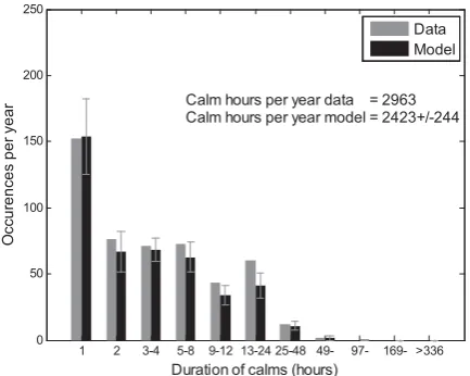
[image:3.595.48.280.284.410.2]The duration of calms is also important. In system impact studies this will determine where the generation will likely come from and what parts of the grid need particular attention. The duration of the calms also gives a good idea of how well the model captures synoptic variations in wind speed - in the UK long term calm durations typically represent low pressure weather systems passing through. Figure 4 shows how the model and real data can be compared in grouped categories. Relatively short calm periods can be balanced with spinning reserve, whereas longer term calm periods will need additional plants brought online.
1 2 3-4 5-8 9-12 13-24 25-48 49- 97- 169- >336 0
50 100 150 200 250
Duration of calms (hours)
O
cc
u
renc
es
per
y
e
ar Calm hours per year data = 2963Calm hours per year model = 2423+/-244
Data Model
[image:3.595.314.531.467.640.2]4.3 Wind speed variability
The variability is a measure of the rate of change of wind speed. It performs a similar role to the auto-correlation function. The calculation used is as follows:
¦
''
Nn
t tn
tn
W
W
N
t
W
1
1
)
(
(2)Where
W
(
'
t
)
is the change in magnitude of wind speed, tn is the nth simulation time step and ǻt is the time horizon.On short time scales of up to about 4 hours ahead a good approximation to the variability is useful so that reserve back-up is accurately modelled in power system impact studies: a CCGT has a start-up time of 4 hours [12]; and accurate representation shows that the model incorporates the correct level of uncertainty in wind speeds for each time step of the simulation. Figure 5 shows a close match, the diurnal wind speed variations can also be noted when the time scale is expanded. Variability is reduced at 24 hour intervals as the corresponding hours are influenced by the diurnal trends.
0 5 10 15 20
0 0.2 0.4 0.6 0.8 1 1.2 1.4 1.6 1.8 2
Time horizon (hours)
M
e
a
n
ab
sol
u
te
c
h
ange
in
w
ind
speed
(
m
/s
)
[image:4.595.315.534.101.276.2]Data Model
Figure 5 A typical wind speed variability curve
In Figure 6 the change in wind speeds at a 4 hour ahead time horizon are looked at. This determines how well the model simulates changes in wind speed. In the example the model under predicts some of the larger changes in wind speed and in impact studies this means some of the more extreme power scenarios where flows are altering rapidly would not be given the weight they deserve when making planning decisions.
0 1 2 3 4 5 6 7
100 101 102 103 104
Absolute wind speed change (m/s)
O
ccu
re
nce
s pe
r yea
r
[image:4.595.55.270.360.533.2]Data Model
Figure 6 Distribution of absolute wind speed change over 4 hours
4.4 Wind speed volatility
The volatility is a measure of the change in wind speed expected at any given wind speed. The volatility of the wind is important particularly at below rated operation of wind turbines, as any variations in wind speed will result in changes of power output. The power output is proportional to the cube of the wind speed, so the effect of volatility is amplified while below rated wind speed, resulting in large power fluctuations. These will need to be balanced by spinning reserve. In Figure 7 the volatility increases slightly with wind speed, the model on the other hand has an approximately steady volatility; the important section to mimic correctly is at below rated wind speeds, 4-15 m/s.
0 2 4 6 8 10 12 14 16 18 20
0.5 1 1.5 2 2.5 3
Wind speed
M
ea
n abs
ol
ut
e
1-hour
c
hang
e
data model
[image:4.595.315.534.495.664.2]4.2 Look ahead RMSe
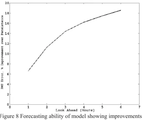
The RMS look ahead error is a measure of the predictive power of the model: it demonstrates how well the model may be used to forecast future wind speeds.
[image:5.595.310.539.94.222.2]At each look ahead hour the difference between the predicted and the actual wind speed across the entire data set is calculated, squared, summed then square rooted to get the RMSe. To determine the effectiveness of the model a comparison is made with predictions from a persistence model. Figure 8 shows an example where the performance of the model improves compared to the persistence prediction with increasing look ahead times.
Figure 8 Forecasting ability of model showing improvements over persistence predictions
4.5 Correlation between sites
As well as temporal correlation weather systems also result in spatial correlation. This is often ignored in wind field models by either falsely assuming sites can be simulated individually without reference to each other or treating large areas as having just one average wind speed at any given time. In reality this is not the case and spatial correlations can have an impact on the stability of the power system. For example, if power flows typically run in a north-south direction and on a particular day there is abnormally high winds in the north and low winds in the south this could overload certain transmission lines and lead to curtailment of wind plants, potentially reducing revenue for these generators or costing the transmission operator in balancing fees [1].
The method proposed here to confirm that spatial correlation has been correctly included is to measure the correlation between pairs of sites at different distances from each other, and plot to compare the model with real data. Figure 9 shows how sites close together are well correlated whereas sites further apart are only weakly correlated. The reason behind this is that sites close together are experiencing the same weather conditions.
0 200 400 600 800 1000
-0.2 0 0.2 0.4 0.6 0.8
Distance Apart, km
Correl
ation, Pairs of
Sit
es
De-trended Data and Model
[image:5.595.44.288.252.459.2]Data Model
Figure 9 Graph showing correlation between pairs of sites, with decreasing correlation with increasing separation
The implication of this is that regions of the grid will experience high or low wind output at the same time, meaning flows into and out of these regions will be affected. Also, this shows the advantage of spreading wind plants further apart, as the uncorrelated plants can act to balance out the power output, reducing the overall variability of the wind plants.
5 Conclusion
A number of techniques have been described that can be used to validate wind field models for power system impact studies. The implication of failing to validate models using each of these methods is described along with the method.
The criteria required of a wind field model for different power system impact studies will vary depending on what is being looked at, however a full validation, like has been described here, is advised for all wind field models so that they are not used inappropriately and false conclusions reached.
Acknowledgements
The work described in this paper was supported in part by EPSRC PhD funding at the Doctoral Training Centre in Wind Energy Systems at the University of Strathclyde. The supply of meteorological data is gratefully acknowledged from the British Atmospheric Data Centre.
References
[1] T. Ackermann, “Wind Power in Power Systems,”
John Wiley & Sons, Chichester, (2005)
[2] T. Aigner, T. Gjengedal, “Detailed wind power
production in northern Europe,” Renewable Energy 2010 Proceedings, , Yokohama, Japan, (2010)
[5] P. R. J. Campbell, “Short term wind energy forecasting,” Proc. IEEE Canada Electrical Power Conf., pp. 342–346, (2007)
[6] E. Denny, M. O’Malley, “Wind generation, power
system operation, and emissions reduction,” IEEE Trans. Power Syst., volume 21, pp. 341–347, (2006)
[7] D. Hill, D. McMillan, K. Bell, D. Infield,
“Application of Auto-regressive Models to UK Wind Speed Data for Power System Impact Studies,” IEEE Transaction on Sustainable Energy,volume 3, pp. (2012)
[8] D.C. Hill, D. McMillan, K.R. Bell, D. Infield,
“Application of Auto-regressive Models to UK Wind Speed Data for Power System Impact Studies”, accepted for publication in July 2012 IEEE Transactions on Sustainable Energy
[9] A. Gerber, M. Qadrdan, M. Chaudry, J. Ekanayake, N. Jenkins, "A 2020 GB transmission network study using dispersed wind farm power output", Renewable Energy, vol. 37, pp. 124-132, 2012
[10] N.B. Negra, O. Holmstrøm, B. Bak-Jensen, P.
Sørensen, “Model of a synthetic wind speed time series generator”, Wind Energy, vol. 11, no. 2, pp. 193–209, March/April 2008
[11] G. Sinden, “Characteristics of the UK wind resource: Long-term patterns and relationship to electricity demand,” Energy Policy,volume 35, pp. 112-127 (2007)
[11] G. Sinden, “Characteristics of the UK wind resource: Long term patterns and relationship with electricity demand”, Energy Policy, no. 35, pp.112-127, 2006
[12] S. Sturt, G. Strbac, “Time-series modelling of power output for large-scale wind fleets,” Wind Energy,volume 14, pp. 953-966, (2011)
[12] A. Sturt, G. Strbac, “Time series modelling of power output for large-scale wind fleets”, accepted for publication in Wind Energy.