Comparison of multiple power amplification types for power hardware-in-the-loop applications

Comparison of multiple Power Amplification types

for Power Hardware-in-the-Loop Applications

Felix Lehfuss and

Georg Lauss

Vienna, Austria

<felix.lehfuss;georg.lauss>@ait.ac.at

Panos Kotsampopoulos and

Nikos Hatziargyriou

Engineering

National Technical University of Athens Athens. Greece

<Kotsa;nh>@power.ece.ntua.gr

Paul Crolla and

Andrew Roscoe

Department of Electronic and Electrical Engineering

University of Strathclyde Glasgow, Scotland paul.crolla@eee.strath.ac.uk

Abstract—This Paper discusses Power Hardware-in-the-Loop simulations from an important point of view: an intrinsic and integral part of PHIL simulation – the power amplification. In various publications PHIL is discussed either in a very theoretical approach or it is briefly featured as the used method. In neither of these publication types the impact of the power amplification to the total PHIL simulation is discussed deeply. This paper extends this discussion into the comparison of three different power amplification units and their usability for PHIL simulations. Finally in the conclusion it is discussed which type of power amplification is best for which type of PHIL experiment.

Keywords: Power Hardware-in-the-Loop (PHIL), Power Amplification;

I. INTRODUCTION

Power Hardware-in-the-Loop (PHIL) is a simulation technology that has received a massive growth of interest in the last couple of years. PHIL is an extension to the commonly known Hardware-in-the-Loop (HIL) technology [1]. HIL simulations have proven to be a very useful tool that allows testing the device in a simulated environment. This testing can be done from very early stages of development up to the final product. Moreover the HIL approach inherently allows the examination of the transient response of a yet-to-be-built system and/or device. A classical HIL experiment typically consists at least out of a Real-Time-System (RTS) a D/A conversion, a Hardware under Test (HuT) and some measurement devices or A/D conversion to close the HIL loop [1][2][4]. However HIL simulations are limited to the power range of the D/A conversion modules used. If the HuT either consumes or produces power out of the range of the A/D conversion the classical HIL approach cannot be applied. In order to be able to carry out such a simulation with a “power

HuT” one has to follow the approach of PHIL simulation which introduces a Power Amplification (PA) between the RTS and the HuT. Figure 1 depicts an overview of the signal flow of a PHIL simulation through the involved components.

This introduction of a PA, enables crossing the barrier of power range that is represented in the A/D conversion modules used. However, this does not come without a drawback, as the introduction of the PA comes along with the introduction of an Additional Control Loop (APL). This APL introduced between the RTS and the HuT would not be existent in the real system and, in dependency of the simulated system, can cause the system simulated using PHIL to be unstable even if the real system would be stable [1][2][3].

Ideally the PA between the RTS and the HuT should have a unity gain with infinite bandwidth and zero time delay. Praxis, however, despite all dreams of ideality, proves that a PA has none of these three wishful attributes. Every real PA will introduce errors in dependency of its real dynamic behavior. The magnitude of these introduced errors massively affects the fidelity and the validity of the simulation [3][9].

The closed loop of a PHIL simulation consists out of at least the following elements: A time delay introduced by the discrete character of the RTS as every RTS typically has a discrete character. As discussed above no real PA will be ideal, the dynamic behavior of the HuT, being the element of testing-interest for most PHIL simulations. The measurement, which will be necessary in order to close the loop, the simulated system itself, which will have a behavior that is very well known as the corresponding models, were designed accordingly. The discussed ACL brings stability issues to a system that might be fully stable in a “non-simulation” environment such as a pure hardware test. The stability issues that come along with the ACL have been reported in various papers and the common sense that can be found in various publications is that the Interface Algorithm (IA) has to cope with this issue. [1][11][16]

The work leading to this approach received funding from the European Community's Seventh Framework Program (FP7/2007-2013) DERri under grant agreement no 228449. Further information is available at the website: www.der-ri.net.

Figure 1: Signal flow overview of a PHIL simulation

Amplifier

Applied

Pulse Function

singe step

response

Figure 2: Typical Test setup for the characterization of a Power Amplification Unit

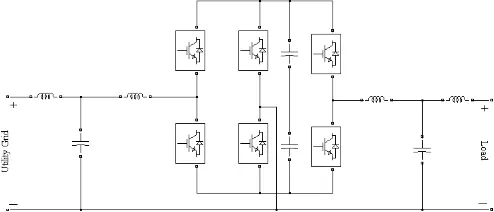
Figure 3: Simplified diagram of the 3-leg AC-DC-AC converter

Most PHIL IA can be implemented either as current controlled or voltage controlled IA. The type of IA is sometimes determined by the equipment one has available, as usually both power amplification units - voltage type and current type - are not available. An exception to this, as later discussed are switched mode amplifiers. In strong dependency of the use case one wants to evaluate using PHIL, either current type or voltage type power amplification is better to be used. This paper focuses only on voltage type power amplification for PHIL.

The dynamic behavior of the PA is a specific system- element that introduces the most instability issues into a PHIL simulation, assuming one uses state of the art measurement devices to close the PHIL loop. The design of a PHIL experiment as well as the choice of the IA massively depends on the PA one has available. This paper takes advantage of the fact that the authors have three different PA units available, a Switched Mode Amplifier, a Generator Type Amplification and a Linear Power Amplification Unit and is structured as follows: in the second section three different power

amplifications are described and discussed individually, in the third section the applicability of each power amplification unit is discussed. In the conclusion a guideline which power amplification is best for which type of PHIL experiment is given.

II. POWER AMPLIFICATION

For PHIL simulation the stability evaluation before performing the experiment is an essential part at the current state of development for PHIL simulation. In order to be able to carry out a pre-experimental stability evaluation for the PHIL experiment it is necessary to have a system description of every component in the control loop available. The proposed method in this paper is to use Transfer functions which can be derived out of a step response that could be acquired using a test setup as depicted in Figure 2. Three different Power Amplifications are described subsequently.

A. Switched Mode Power Amplification

Switched-mode devices have been commonly used as power amplifiers for PHIL simulation even at the MW range [17]. An AC/DC/AC converter, which consists of a front-end rectifier and a back-end inverter, allows coupling to the utility grid, and voltage or current source operation. In this way power can be provided to the HuT from the utility grid, or can be absorbed from the HuT and injected to the grid. The Real-Time Simulator sends the reference low level signal to the inverter (voltage or current), which applies to the HuT by using suitable control algorithm. In addition, an operation as a DC amplifier is possible.

Several control approaches (PI, PID, predictive control etc) [18], [19] and configurations of the output filter (L-C or L-C-L) have been proposed according to the application. Different topologies of the semi-conductors are used for three phase amplifiers: 3-leg DC/AC inverters, but also 4-leg inverters to allow unbalanced operation. In addition, a high switching frequency of the semi-conductors is proposed in-order to enable tracking of the fast dynamics of the RTS [19].

1) Presentation and characterization

A PHIL simulation environment focusing on DER devices is operated in NTUA. The RealTime Simulator of NTUA is a rack of the RTDS® with a typical simulation time-step of 50 µsec [5] and the HuT comprises the laboratory microgrid [20].

(a) (b)

Figure 4: (a) Torque control system (b) Command to measured value response of the phase loop and frequency loop: hand-tuned parameters

be easily improved and fully modified by the user. Voltage and current measurements are available in the same Matlab/Simulink model, which are used to provide the feedback signal, that represents the response of the HuT, to the RTS. Several analog I/Os equipped with A/D and D/A converters are available which make possible the communication with the RTDS. Therefore the aforementioned AC/DC/AC converter is suitable for working as a Power Interface in PHIL simulation.

A key issue for the evaluation of both stability and accuracy of PHIL simulation is the derivation of the Transfer Function of the Power Interface and more specifically of the Power amplification. Typically for Switched-mode amplifiers the Transfer Function is derived from the introduced time-delay and output filter of the converter. Therefore the Transfer Function of the Amplifier is [2] [9]:

f sT

AMP e T

T ₌ − d1_⋅ (1)

Where Td1 is the time-delay and Tf is the Transfer Function

of the output filter. The time-delay introduced by the power amplifier is measured in steady-state conditions (Figure 5). Improving the control algorithm of the amplifier can result in a reduction of the time-delay. The Transfer Function of the output filter is derived approximately by performing harmonic measurements on the PWM voltage before the output filter and the sinusoidal voltage after the filter. A second order filter is considered:

2 2

2 2

2 2

2

2 _{1,42 750 (2 750)}

) 750 2 ( 2

1 1 2 1

1

⋅ + ⋅ ⋅ ⋅ +

⋅ =

+ ⋅ ⋅ + =

+       +       =

π π

π ω

ω ξ

ω

ξ s s s s s

f s f T

n n n

res res

f

where ωn is the resonance angular frequency and ξ the

damping ratio.

2) Use Case

A low voltage distribution grid is simulated in the Real Time Simulator and the laboratory microgrid is the HuT. The low voltage microgrid comprises a PV generator, a small Wind Turbine, battery energy storage and controllable loads. The PV generators, the Wind Turbine and the battery unit are connected to the utility grid or to the power amplifier via fast-acting DC/AC power converters. Interactions between the

micro-sources and the simulated distribution grid are performed (e.g. voltage variation due to PVs production) in-order to study the integration of DER to distribution networks.

B. Generator Type Power Amplification

A further method for power amplification in a Real Time-PHIL environment is through the use of a three phase synchronous generator driven by a DC motor and separate rotating exciter system. In this set up a real-time simulator runs a simulation of a power system with a Point of Common Connection (PCC) with the output of the synchronous generator. The generator is controlled in torque mode. Full information on the discussed set-up can be found in [13].

1) Characterisation

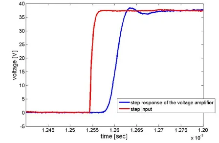
The closed loop transfer function for the motor torque input was derived in [10]. The derived control parameters for the PIDA (proportional-integral-differential-acceleration) controllers are shown below in equations. This type of control is unusual, however it was found that without the acceleration element the controller output was unstable.

The right hand loop (shown in Figure 4(a) above) is a conventional frequency control loop enabling the frequency output of the generator to be matched with the target from the model, the left hand loop deals with locking the phase of the generator output with the simulation.

(

)

(

)

(

)

(

)

D C HL H D C F F + = + + + 1 1 1 1 1 (3) bs RP) +HL))F}]Q' D(H/( +C { +HL))} D(H/( [{C +QC R)/( +HL))F}]Q' D(H/( +C +HL))}/{ D(H/( [{C (QC F F P F F P + = 1 1 1 1 1 1 1 1 1 (4)

2) Response of the Generator

The phase tracking of the output of the prime mover has been shown to be between 10-15° with 5 Hz/s rate of change of frequency. Phase tracking is much better than this when considering less dynamic scenarios. In Figure 4 (b) it is possible to see the phase and frequency response of the generator controller at different frequencies.

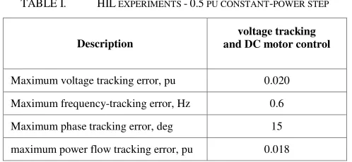
The error response of the generator to load change steps of 0.5 p.u. has been shown in detail in [11][12] and a summary of the results are presented in TABLE I. below. These represent the minimum possible errors after performing the ‘lambda-tuning’ process (a variant of internal model control tuning [10]). Performing larger steps in restive load, e.g. 0.8 or 1 p.u. steps are almost impossible to track with this type of system as the ROCOF would be very large. Further the larger the ROCOF the harder the generator is driven to change speed potentially risking damage to the generator. Therefore smaller changes in resistive load are easier and safer to track.

For load step changes with an inductive or capacitive element then it is the time delay in the automatic voltage regulator (AVR) that is dominant on the tracking of the real output to the simulated one. It is expected that smaller step changes in reactive power will be more easily tracked by the hardware than larger ones.

TABLE I. HIL EXPERIMENTS -0.5 PU CONSTANT-POWER STEP

Description

voltage tracking and DC motor control

Maximum voltage tracking error, pu 0.020

Maximum frequency-tracking error, Hz 0.6

Maximum phase tracking error, deg 15

maximum power flow tracking error, pu 0.018

3) Use Case

This system was developed initially to link a larger or more complicated power system simulation with a real hardware power system/microgrid see for examples [10][12][13]. The use of this is to study the effects that larger system events have on smaller local power systems and conversely to study the effects small power system events can have on the larger system (if a summation is used). These studies are necessary

with the increased use of complicated power electronic connected generators and loads within the distribution system.

C. Linear Power Amplification

The PHIL simulation environment at the AIT focuses on the simulation of DER devices with a further specialization on photovoltaic inverters. The laboratory consists out of an OPAL RT Real Time Simulator [14] and of three Spitzenberger & Spieß PAS 1000 Linear Power Amplifier [15] as well as of multiple measurement equipment.

1) Description

The topology of the linear amplification stage is consisting of multiple linear MOSFET’s controlled in parallel in such way that the characteristics are adequate to a discrete MOSFET operated in the linear region. Thus, the key characteristics of the used linear amplifier are defined and identified as followed. The slew rate is given to > 52 V / µs and the rise time at nominal voltage (230 Vrms) is less than 5 µs. The effective

bandwidth is set to 0 - 15 kHz and the graph of a typical step response is highlighted in Figure 6. Furthermore, the total harmonic distortions at typical operation (nominal load, 270 V range and 0.5 – 2 kHz) is set to be typically 0.3% [15].

The control of the amplifier can be either executed with the help of 2 internal oscillators or via an external input signal. This external analogue voltage signal is used for the PHIL testing system having a dedicated input range of maximum 5 Vp (3.535 Vrms). The amplifier features 2 different output

ranges (135 V and 270 V), which gives expedient usability for common low voltage experiments. Thus, having activated the 270 V range, which is most commonly used at PHIL tests, an input voltage signal of 3.011 Vrms results in a driven output

voltage of 230 Vrms.

The forward branch of the PHIL environment used at the AIT consists out of the analogue output of the OPAL RT RTS and the Voltage Amplification. In some cases an additional anti-aliasing filter is introduced to reduce the stepped shape of the RT signal due to the discrete character of the RTS.

The feedback branch of the PHIL environment consists out of a current measurement, and the analogue inputs of the OPAL RT RTS. For some applications an additional feedback filter is introduced in order to stabilize the PHIL experiment [16].

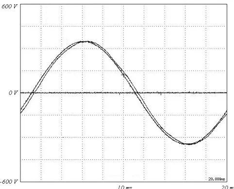
2) Response of the Generator

In order to be able to obtain the transfer function of the PA in use the PA was excited with a pulse function out of which a single step was evaluated. The single step response of the Spitzenberger & Spieß PAS 10000 [15] can be seen in Figure 6. The result of this single step evaluation was then compared to other step responses out of the pulse function to verify the results.

The transfer function of the linear voltage amplifier basically resembles a PT2 system with a time delay of 4µs. The linear character of the used voltage amplification allows more of a straight forward implementation than it would be available with other power amplification units

3) Use Case

At the AIT there is a high level of expertise regarding PV Inverters available. Thus a grid connected PV Inverter is a very promising use case for future PHIL applications. Figure 7 shows such a grid connected PV Inverter as possible PHIL use case. The advantage of the PHIL application in this particular use case is the high adaptability of the simulated grid. It is possible to test a single HuT in different low voltage grids as well as different grid condition of the same model. A more detailed description of this use case can be found in [21] One has to differentiate between active HuT and passive HuT. This use case provides an active HuT as the dc coupling to the PV-Inverter is implemented using a PV array simulator which is not controlled by the RTS. The control of the active load is determining the AC current which then goes into the feedback loop of the simulated system.

In high contrast to that, passive components - as e.g. protection devices - have to be run at certain defined operation conditions and thereby require an amplification of both voltage and current.

.

Figure 6: Step response of the Spitzenberger & Spieß PAS 10000 Linear Power Amplifier

Figure 7: PHIL Use Case: Grid connected PV Inverter [21]

III. APPLICABILITY OF THE POWER AMPLIFICATION UNITS

1) Swiched mode amplifiers

Switched-mode amplifiers represent a higher level of time-delay and lower accuracy (e.g. introduction of noise) than linear amplifiers. On the other hand, they are less expensive and they can quite easily be constructed even at MW ranges and present greater flexibility. For example, the same amplifier can operate both as voltage and current amplifier by applying suitable control algorithm.

2) Syncronous generator amplifiers

The use of a synchronous generator as the power amplifier is relevant to performing research and testing where a balanced three phase supply is required. E.g. testing a three phase inverter or motor-drive, or studying the interaction between devices connected to different single phases.

3) Linear amplifier

The biggest advantage of a linear voltage amplifier is his very high dynamic performance. The short time delay, and comparable easy transfer function, introduced to a PHIL simulation enables the engineer to use a more straight forward interface topology with less stability issues.

IV. CONCLUSION

This paper presented three different types of voltage type power amplification units which are used for PHIL applications. The dynamic behavior of each power amplifier is discussed within the scope of PHIL. The presented comparison is not intended to rate which power amplifier is the best but to give an overview of what type of PHIL experiment can be achieved with which type of power amplifier.

For the proper characterization of amplification units it is mandatory to verify the hardware one has available. The characteristics presented in this paper are not necessarily representative for other power amplification units of the same type. The authors strongly recommend a individual characterization of the amplifier in use as the dynamic behavior of the amplifier is a crucial element of every PHIL application.

In this paper three different types of power amplification units have been discussed in detail. Their dynamic behavior was shown and a resulting statement was given about the benefits of each power amplification unit.

REFERENCES

[1] W. Ren, M. Steuer and T. L. Baldwin,Improve the Stability and the Accuracy of Power Hardware-in-the-Loop Simulation by Selecting Appropriate Interface Algorithms“, IEEE Transactions on Industry Applications, Vol. 44, No. 4, pp. 1286-1294, July 2008.

Digital Simulators", IEEE Transactions on Power Delivery, vol. 26, no. 2, pp. 1221–1230, April 2011

[3] A. Viehweider, G. Lauss, F. Lehfuss, Stabilization of Power Hardware-in-the-Loop simulations of electric energy systems, Simulation Modelling Practice and Theory, Volume 19, Issue 7, August 2011, Pages 1699-1708, ISSN 1569-190X, 10.1016/j.simpat.2011.04.001.

[4] A. Monti, H.. Figueroa, S. Lentijo, X. Wu and R. Dougal, ”Interface Issues in Hardware-in-the-Loop Simulation” , IEEE Electric Ship Technologies Symposium ESTS, pp. 39- 45, July 2005.

[5] RTDS Technologies: http ://www.rtds.com

[6] T. Loix, S. de Breucker, P. Vanassche, J. van den Keybus, J. Driesen and K. Visscher, “Layout and per-formance of the power electronic converter platform for the VSYNC project”, Proceedings of the IEEE Po-wertech conference, , Bucharest, Romania, 2009

[7] Triphase: http://www.triphase.com

[8] Jacobina C.B., Oliveira T.M., da Silva E.R.C., “Control of the Single-Phase Three-Leg AC/AC Converter”, IEEE Transactions on Industrial Electronics, vol. 53, no.2, pp. 467-476, 2 April 2006

[9] W. Ren, “Accuracy Evaluation of Power Hardware-in-the-Loop (PHIL) Simulation”, PhD Thesis The Florida State University, 2007.

[10] Lennartson, B., Kristiansson, B.: ‘Evaluation and tuning of robust PID controllers’, IET Control Theory Appl., vol. 3, pp. 294–302, 2009 [11] M Hong, S. Horie, Y. Miura, T. Ise and C. Dufour, “A Method to

Stabilize a Power Hardware-in-the-loop Simulation of Inductor Coupled Systems”, International Conference on Power Systems Transients, Kyoto (Japan), June 2009.

[12] Roscoe, A.J.; Mackay, A.; Burt, G.M.; McDonald, J.R.; , "Architecture of a Network-in-the-Loop Environment for Characterizing AC Power-System Behavior," Industrial Electronics, IEEE Transactions on , vol.57, no.4, pp.1245-1253, April 2010.

[13] Roscoe, A.J.; Elders, I.M.; Hill, J.E.; Burt, G.M.; , "Integration of a mean-torque diesel engine model into a hardware-in-the-loop shipboard network simulation using lambda tuning," Electrical Systems in Transportation, IET , vol.1, no.3, pp.103-110, September 2011. [14] OPAL RT Technologies, http:// www.opal-rt.com

[15] Spitzenberger & Spiess GmbH, http ://www.spitzenberger.de

[16] Lauss, G.; Lehfuss, F.; Viehweider, A.; Strasser, T.; , "Power hardware in the loop simulation with feedback current filtering for electric systems," IECON 2011 - 37th Annual Conference on IEEE Industrial Electronics Society , vol., no., pp.3725-3730, 7-10 Nov. 2011 doi: 10.1109/IECON.2011.6119915.

[17] M. Sloderbeck, F. Bogdan, J. Hauer, L. Qi, and M. Steurer “The addition of a 5 MW variable voltage source to a hardware-in-the loop simulation and test facility”, in Proc. EMTS, Philadelphia, PA, Aug. 12–13, 2008. [18] V. Karapanos, S. de Haan, K. Zwetsloot, "Real Time Simulation of a

Power System with VSG Hardware in the Loop", Proc. IEEE Industrial Electronics Society IECON’2011, Australia, November 2011

[19] A. Benigni, A. Helmedag, A. Abdalrahman, G. Piłatowicz, A. Monti, “FlePS: A power interface for Power Hardware In the Loop”, Proceedings of the 2011-14th European Conference on Power Electronics and Applications (EPE 2011)

[20] Hatziargyriou N., “Microgrids [guest editorial]”, IEEE Power and Energy Magazine, Volume 6, Issue 3, May-June 2008 Page(s): 26 – 29 [21] A. Viehweider, F. Lehfuss, G. Lauss, „Power Hardware-in.the-Loop