A new index of financial conditions

(1)

A New Index of Financial Conditions

Gary Koop

University of Strathclyde

Dimitris Korobilis

y

University of Glasgow

July 4, 2014

Abstract

We use factor augmented vector autoregressive models with time-varying coefficients and stochastic volatility to construct a financial conditions index that can accurately track expectations about growth in key US macroeconomic variables. Time-variation in the model’s parameters allows for the weights at-tached to each financial variable in the index to evolve over time. Furthermore, we develop methods for dynamic model averaging or selection which allow the financial variables entering into the financial conditions index to change over time. We discuss why such extensions of the existing literature are important and show them to be so in an empirical application involving a wide range of financial variables.

Keywords: Bayesian model averaging; dynamic factor model; dual Kalman

filter; forecasting

JEL Classification:C11, C32, C52, C53, C66

We want to thank Gianni Amisano, Klemens Hauzenberger, Sylvia Kaufmann, Michael McCracken, Francesco Ravazzolo, and Christian Schumacher for helpful comments. Special acknowledgements to Barbara Rossi for her extensive and insightful suggestions. Finally we want to thank participants at: the 21th Symposium of the Society for Nonlinear Dynamics and Econometrics in Milan; the Conference Forecasting Structure and Time Varying Patterns in Economics and Finance in Rotterdam; the 7th International Conference on Computational and Financial Econometrics in London, and seminar attendees at Birkbeck College, Norges Bank, and Univesité de Rennes 1. This research was supported by the ESRC under grant RES-062-23-2646.

y_{Corresponding author. Address: University of Glasgow, Adam Smith Business School, Gilbert}

(2)

1 Introduction

The recent financial crisis has sparked an interest in the accurate measurement of financial shocks to the real economy. An important lesson of recent events is that financial developments, not necessarily driven by monetary policy actions or fundamentals, may have a strong impact on the economy. The need for policy-makers to closely monitor financial conditions is clear. In response to this need, a recent literature has developed several empirical econometric methods for constructing financial conditions indices (FCIs). FCIs are used for several purposes. For instance, they can be used to identify periods when financial conditions suddenly deteriorate (e.g., Lo Duca and Peltonen, 2013), assess credit constraints or forecast economic developments. An FCI summarizes in one single number information from many financial variables. Many financial institutions (e.g. Goldman Sachs, Deutsche Bank and Bloomberg) and policy-makers (e.g. the Federal Reserve Bank of Kansas City) produce closely-watched FCIs. Estimation of such FCIs ranges from using simple weighted averages of financial variables through more sophisticated econometric techniques. An important recent contribution is Hatzius, Hooper, Mishkin, Schoenholtz and Watson (2010) which surveys and compares a variety of different approaches. The FCI these authors propose is based on simple principal components analysis of a very large number of quarterly financial variables. Other recent notable studies in this literature include English, Tsatsaronis and Zoli (2005), Balakrishnan, Danninger, Elekdag and Tytell (2008), Beaton, Lalonde and Luu (2009), Brave and Butters (2011), Gomez, Murcia and Zamudio (2011) and Matheson (2011).

In this paper our goal is to accurately monitor financial conditions through a single latent FCI. The construction and use of an FCI involves three issues: i) selection of financial variables to enter into the FCI, ii) the weights used to average these financial variables into an index and iii) the relationship between the FCI and the macroeconomy. There is good reason for thinking all of these may be changing over time. Indeed, Hatzius et al (2010) discuss at length why such change might be occurring and document statistical instability in their results. For instance, the role of the sub-prime housing market in the financial crisis provides a clear reason for the increasing importance of variables reflecting the housing market in an FCI. A myriad of other changes may also impact on the way an FCI is constructed, including the change in structure of the financial industry (e.g. the growth of the shadow banking system), changes in the response of financial variables to changes in monetary policy (e.g. monetary policy works differently with interest rates near the zero bound) and the changing impact of financial variables on real activity (e.g. the role of financial variables in the recent recession is commonly considered to have been larger than in other recessions).

(3)

methods to account for time-variation. Furthermore, many FCI’s are estimated ex post, using the entire data set. So, for instance, at the time of the financial crisis, some FCIs will be based on financial variables which are selected after observing the financial crisis and the econometric model will be estimated using financial crisis data. The major empirical contribution of the present paper is to develop an econometric approach which allows for different financial variables to affect estimation of the FCI, with varying (or zero, when not selected) weight each. In this manner, we develop an econometric tool that explicitly takes into account the fact that each financial crisis has different causes, and is transmitted to the real economy with varying intensity.

Following a common practice in constructing indices, we use factor methods. To be precise, we use extensions of Factor-augmented VARs (FAVARs) which jointly model a large number of financial variables (used to construct the latent FCI) with key macroeconomic variables. Following the recent trend in macroeconomic modelling using VARs and FAVARs (Primiceri, 2005; Korobilis, 2013) we work with time-varying parameter FAVARs (TVP-FAVARs) which allow coefficients and loadings to change in each period. TVP-FAVARs have enjoyed increasing popularity for forecasting macroeconomic variables (see, among others, Eickmeier, Lemke and Marcellino, 2011a and D’Agostino, Gambetti and Giannone, 2013).

Additionally, we work with a large set of (TVP-) FAVARs that differ in which financial variables are included in the estimation of the FCI. Faced with a large model space and the desire to allow for model change, we follow Koop and Korobilis (2012) and use efficient methods for Dynamic Model Selection (DMS) and Dynamic Model Averaging (DMA). These methods forecast at each point in time with a single optimal model (DMS), or reduce the expected risk of the final forecast by averaging over all possible model specifications (DMA). We implement model selection or model averaging in a dynamic manner. That is, DMS chooses different financial variables to make up the FCI at different points in time. DMA constructs an FCI by averaging over many individual FCIs constructed using different financial variables. The weights in this average vary over time.

From an econometrician’s point of view, there is also growing theoretical evidence in favor of our modelling strategy. Boivin and Ng (2006) show that using all available data to extract factors (the FCI in our case) is not always optimal in factor analysis, thus providing support for implementing DMA/DMS to construct our FCI. Additionally, there is much econometric evidence in favor of structural instabilities in the coefficients or loadings of macroeconomic and financial factor models; see, among others, Banerjee, Marcellino and Masten (2006) and Bates, Plagborg-Møller, Stock and Watson (2013).

(4)

algo-rithms or complex numerical methods, all of which are computationally extremely demanding in high dimensions. With our large model space, and our wish to implement recursive forecasting, it is computationally infeasible to use such methods. Therefore, our major econometric contribution in this paper lies in the development of fast estimation methods which are based on the Kalman filter and smoother and are simulation-free. When dealing with the FAVAR with constant parameters, our algorithm collapses to the two-step estimator for dynamic factor models of Doz, Giannone and Reichlin (2011). In the case of estimating models with time-varying parameters and stochastic volatility (TVP-FAVARs), our algorithm provides an extension of Doz, Giannone and Reichlin (2011).

Our results indicate that financial variables do have predictive power for macro-economic variables (GDP growth, inflation and unemployment). Additionally, time variation in the parameters is important for providing accurate short-run forecasts. Finally, model averaging and/or selection also result in the improvement of forecast accuracy over using a single model with all the available financial variables. In the remainder of the paper we examine all these issues in depth, and we provide evidence by using different forecast metrics and by conducting several robustness checks.

In particular, in the next section we introduce our modeling framework and sketch the features of our novel estimation algorithm (complete details are provided in the Technical Appendix), plus we describe how we implement DMA or DMS methods in the face of the large number of models we work with. In Section 3 we present our data, estimates of different FCIs, and results of a recursive forecasting exercise which is the main tool for evaluating the performance of our FCI. Section 4 concludes the paper. An empirical appendix provides an extensive sensitivity analysis to various aspects of our specification.

2 Factor Augmented VARs with Structural

Instabili-ties

2.1 The TVP-FAVAR Model and its Variants

Let xt (for t = 1; :::; T) be an n 1 vector of financial variables to be used in

constructing the FCI. Letytbe ans 1vector of macroeconomic variables of interest.

In our empirical workyt = ( t; ut; gt)0 where t is the GDP deflator inflation rate,ut

is the unemployment rate, gt is the growth rate of real GDP. The p-lag TVP-FAVAR

takes the form

xt= ytyt+ ftft+vt

yt

ft

=ct+Bt;1 yt 1 ft 1

+:::+Bt;p

yt p

ft p

+"t

(5)

where y_t are regression coefficients, f_t are factor loadings, ft is the latent factor

which we interpret as the FCI, ct is a vector of intercepts, (Bt;1; :::; Bt;p) are VAR

coefficients and ut and "t are zero-mean Gaussian disturbances with time-varying

covariances Vt and Qt, respectively. We adopt the common identifying assumption

in the likelihood-based factor literature1 _that_V

tis diagonal, thus ensuring thatvtis

a vector of idiosyncratic shocks andftcontains information common to the financial

variables. This model is very flexible since it allows all parameters to take a different value at each timet. Such an assumption is important since there is good reason to believe that there is time variation in the loadings and covariances of factor models which use both financial and macroeconomic data (see Banerjee, Marcellino and Masten, 2006). For recent discussions about the implication of the presence of structural breaks in factor loadings, the reader is referred to Breitung and Eickmeier (2011) and Bates, Plagborg-Møller, Stock and Watson (2013).

Following the influential work of Bernanke, Boivin and Eliasz (2005) our factor model in (1) consists of two equations: one equation which allows us to extract the latent financial conditions index (FCI) from financial variables xt; and

one equation which allows to model the dynamic interactions of the FCI with macroeconomic variables yt. This econometric specification is important for two

reasons. First, unlike Stock and Watson (2002) who extract a factor and then use it in a separate univariate forecasting regression, we use a multivariate system to forecast macroeconomic variables using the FCI. Thus, we jointly model all the variables in the system which should allow us to better characterize their co-movements and interdependence. Second, we are able to purge from the FCI the effect of macroeconomic conditions. Thus, the final estimated FCI reflects information solely associated with the financial sector.

It is worth digressing to expand on the manner in which we include macro-economic variables in our model. Including yt on the right-hand side of the first

equation of (1) is intended solely to ensure the FCI reflects only financial conditions. This is also done in Hatzius et al. (2010) for the same reason. However, it is worth stressing that, by doing this, we are only purging the FCI of the effect of current macroeconomic conditions. Financial variables can also reflect expectations of future macroeconomic variables and we are not purging the FCI of these future expectations. This is an issue common to all FCIs. As a robustness check, our empirical results (see Appendix C) also include a case whereytin the first equation

of (1) is replaced by professional forecasts of macroeconomic variables (which will reflect expectations of future macroeconomic conditions).

Includingyt on the left-hand side of the second equation of (1) is done so as to

provide a metric for evaluating our FCI. That is, in answer to the question: “what makes a good FCI?”, the approach in this paper provides the answer: “it is one which forecastsyt as well as possible”. There are, of course, other possible answers

1_{Some approaches to dynamic factor models which do not use likelihood-based methods allow}

(6)

to this question which would lead to other FCIs. We are not attempting to build a structural model of the economy (e.g. a structural VAR or a DSGE) through the manner we are includingytin (1). Hence, issues which arise with structural models

(e.g. structural VARs often involve an ordering of variables reflecting an assumed causal structure) do not need to be addressed here.

In order to complete our model, we need to define how the time varying parameters evolve. While the specification of all time-varying covariances is discussed in the following subsection, we define here the vectors of loadings

t = ( yt)0; f t

0 0

and VAR coefficients _t = c0

t; vec(Bt;p)0; :::; vec(Bt;p)0 0 to

evolve as multivariate random walks of the form

t= t 1+vt; t = t 1+ t;

(2)

where vt N(0; Wt)and t N(0; Rt). Finally, all disturbance terms presented in

the equations above are uncorrelated over time and with each other.

We call the full model described in equations (1) and (2) the TVP-FAVAR. We also consider several restrictions on the TVP-FAVAR which result in other popular multivariate models:

1. Factor-augmented VAR (FAVAR): This model is obtained from the TVP-FAVAR under the restriction that both tand tare time-invariant (Wt=Rt = 0).

2. Time-varying parameter VAR (TVP-VAR): This model can be obtained from the TVP-FAVAR under the restriction that the number of factors is zero (i.e. ft= 0).

3. VAR: This model is obtained when the number of factors is zero and both t

and _t are time-invariant.

In addition, we consider heteroskedastic (when Vt and Qt are allowed to be

time-varying) and homoskedastic (Vt=V andQt =Q) variants of all models.

2.2 Estimation of a Single TVP-FAVAR

Bayesian estimation of FAVARs (as well as VARs) with time-varying parameters is typically implemented using Markov Chain Monte Carlo (MCMC) methods, which sample from the very complex multivariate joint posterior density of the factor ft

(7)

even in the case of estimating a single FAVAR. When faced with multiple TVP-FAVARs and when doing recursive forecasting (which requires repeatedly doing MCMC on an expanding window of data), the use of MCMC methods is prohibitive.2 In this paper, we use a fast two-step estimation algorithm which vastly reduces the computational burden, and greatly simplifies the estimation of the FCI. Following Koop and Korobilis (2013) we combine the ideas of variance discounting methods with the Kalman filter in order to obtain analytical results for the posteriors of the state variable (ft) as well as the time-varying parameters t = ( t; t). To

motivate our methods, note first that, as long as both the factor,ft, and the loadings, t, in the measurement equation are unobserved, application of the typical Kalman

filter recursions for state-space models is not possible. Therefore, we adapt ideas from Doz, Giannone and Reichlin (2011) and the state-space literature (Nelson and Stear, 1976) and develop a dual, conditionally linear filtering/smoothing algorithm which allows us to estimate the unobserved stateftand the parameters t= ( t; t)

in a fraction of a second.

The idea of using a dual linear Kalman filter is very simple: first update the parameters t given an estimate offt, and subsequently update the factor ft given

the estimate of t. Such conditioning allows us to use two distinct linear Kalman

filters or smoothers,3 _{one for}

t and one for ft. The main approximation involved

is that fet, the principal components estimate of ft based on x1:t, is used in the

estimation of t. Such an approach will work best if the principal component(s)

provide a good approximation of the factor(s) coming from a FAVAR with structural instabilities. A theoretical proof that this is the case is not available for our flexible and highly nonlinear specification. However, given the recent findings of Stock and Watson (2009) and Bates, Plagborg-Møller, Stock and Watson (2013), there is strong theoretical and empirical evidence to believe that this is the case. Empirically, Bates, Plagborg-Møller, Stock and Watson (2013) conduct extensive Monte Carlo experiments and show that principal components can support large amount of time variation in the loading coefficients t. Theoretically, they prove that principal

component estimates of factors are consistent even if there is a substantial amount of time variation or structural change in the factor loadings. For instance, they find that: “deviations in the factor loadings on the order of op(1) [as would occur

with random walk variation in the factor loadings] do not break the consistency of the principal components estimator” (page 290). This is the econometric theory

2_{To provide the reader with an idea of approximate computer time, consider the three variable}

TVP-VAR of Primiceri (2005). Taking 10,000 MCMC draws (which may not be enough to ensure convergence of the algorithm) takes approximately 1 hour on a good personal computer. Thus, forecasting at 100 points in time takes roughly 100 hours. These numbers hold for a single small TVP-VAR, and would be much infeasible for the hundreds of thousands of larger TVP-FAVARs we estimate in this paper.

3_{The other alternative being to use a joint nonlinear filter, e.g. the Unscented Kalman Filter}

(8)

we draw upon to justify use of principal components estimates at this stage in our algorithm.

Error covariance matrices in the multivariate time series models used with macroeconomic data are usually modeled using multivariate stochastic volatility models (see, e.g., Primiceri, 2005), estimation of which also requires compu-tationally intensive methods. In order to avoid this computational burden, we estimate(Vt; Qt; Wt; Rt)recursively using simulation-free variance matrix

discount-ing methods (e.g. Quintana and West, 1988). The Technical Appendix provides complete details. For Vt and Qt we use exponentially weighted moving average

(EWMA) estimators. These depend on decay factors 1 and 2, respectively. Such recursive estimators are trivial computationally. Additionally, the EWMA is an accurate approximation to an integrated GARCH model. Such a feature is in line with authors such as Primiceri (2005) and Cogley and Sargent (2005) who, in the context of macroeconomic VARs, work with integrated stochastic volatility models. The covariance matrices Wt; Rt are estimated using the forgetting factor

methods described in Koop and Korobilis (2012, 2013)4_{which depend on forgetting} factors 3 and 4, respectively. Decay and forgetting factors have very similar interpretations. Lower values of the decay/forgetting factors imply that the more recent observationt 1, and its squared residual, take higher weight in estimatingVt

and Qtcompared to older observations. The choice of the decay/forgetting factors

can be made based on the expected amount of time-variation in the parameters.5 Note that the choice 1 = 2 = 1make Vtand Qtconstant, while 3 = 4 = 1imply thatWt=Rt = 0in which case tand tare constant.

A sketch of the structure of our estimation algorithm is given in the following table.

Algorithm for estimation of the TVP-FAVAR

1. a) Initialize all parameters, 0; 0; f0; V0; Q0

b) Obtain the principal components estimates of the factors,fet

2. Estimate the time varying parameters t givenfet

a) EstimateVt,Qt,Rt, andWtusing VD

b) Estimate t and t, given(Vt; Qt; Rt; Wt), using the KFS

3. Estimate the factorsftgiven t using the KFS

In the table VD stands for “Variance Discounting” and KFS stands for “Kalman filter and smoother”. The steps above can also be considered to be a generalization of

4_{An EWMA estimation scheme can also be applied to these matrices, but due to their large}

dimension we found better numerical stability and precision when using forgetting factors.

5_{Choice of forgetting factors is similar in spirit to choice of prior. Empirical macroeconomists}

(9)

the estimation steps introduced by Doz et al. (2011) for the estimation of constant parameter dynamic factor models. In fact, if we fix all time-varying coefficients and covariances to be constant, our algorithm collapses to the FAVAR equivalent of the two-step estimation algorithm for dynamic factor models of Doz et. al (2011).

Identification in the FAVAR is achieved in a standard fashion by restricting Vt to be a diagonal matrix. This restriction ensures that the factors, ft, capture

movements that are common to the financial variables,xt, after removing the effect

of current macroeconomic conditions through inclusion of the y_tyt term. Further

restrictions usually imposed in likelihood-based estimation of factor models, e.g. normalizing the first element of the loadings matrix to be 1 (Bernanke, Boivin and Eliasz, 2005) are not needed here since the loadings tare identified (up to a sign

rotation) from the principal components estimate of the factor.

2.3 Dynamic Model Averaging and Selection with many

TVP-FAVARs

In this paper, we work with Mj, j = 1; ::; J, models which differ in the financial

variables which enter the FCI. In other words, a specific model is obtained using the restriction that a specific combination of financial variables have zero loading on the factor at timetor, equivalently, that different combinations of columns ofxt

are set to zero. Thus, Mj can be written as

x(_tj) = y_t(j)yt+ f(j)

t f

(j)

t +u

(j)

t

yt

f_t(j) =c (j)

t +B

(j)

t;1

yt 1

f_t(j)₁ +:::+B (j)

t;p

yt p

f_{t p}(j) +" (j)

t

; (3)

where x(_tj) is a subset of xt, and f

(j)

t is the FCI implied by modelMj. Sincext is of

lengthn, there is a maximum of2n 1combinations6_{of financial variables that can} be used to extract the FCI.

When faced with multiple models, it is common to use model selection or model averaging techniques. However, in the present context we wish such techniques to be dynamic. That is, in a model selection exercise, we want to allow for the selected model to change over time, thus doing DMS. In a model averaging exercise, we want to allow for the weights used in the averaging process to change over time, thus leading to DMA. In this paper, we do DMA and DMS using an approach developed in Raftery et al (2010) in an application involving many TVP regression models. The reader is referred to Raftery et al (2010) for a complete derivation and motivation of DMA. Here we provide a general description of what it does.

The goal is to calculate tjt 1;j which is the probability that model j applies

at time t, given information through time t 1. Once tjt 1;j for j = 1; ::; J are

obtained they can either be used to do model averaging or model selection. DMS

(10)

arises if, at each point in time, the model with the highest value for tjt 1;j is used.

Note that tjt 1;j will vary over time and, hence, the selected model can switch over

time. DMA arises if model averaging is done in periodt using tjt 1;j forj = 1; ::; J

as weights. The contribution of Raftery et al (2010) is to develop a fast recursive algorithm for calculating tjt 1;j.

Given an initial condition, 0j0;j for j = 1:; ; :J, Raftery et al (2010) derive a

model prediction equation using a forgetting factor :

tjt 1;j =

t 1jt 1;j

PJ

l=1 t 1jt 1;l

; (4)

and a model updating equation of:

tjt;j =

tjt 1;jfj(DatatjData1:t 1)

PJ

l=1 tjt 1;lfl(DatatjData1:t 1)

; (5)

wherefj(DatatjData1:t 1)is a measure of fit for modelj.7 Many possible measures of fit can be used. Inspired by is a large literature (e.g., among many others, Forni, Hallin, Lippi and Reichlin, 2003) which investigate the ability of financial variables to forecast macroeconomic ones, we focus on the ability of the FCI to forecast yt. Accordingly, we set as a measure of fit the predictive likelihood for the

macroeconomic variables, pj(ytjData1:t 1). is a forgetting factor with 0 < 1 which, similar to the decay/forgetting factors ( 1; 2; 3; 4) used for estimating the error covariance matrices, tunes how rapidly switches between models should occur. Lower values of allow for an increasing amount of switching between the number of variables that enter the FCI each time period. If = 0:99, forecast performance five years ago receives 80% as much weight as forecast performance last period. The case = 1 leads to conventional Bayesian model averaging implemented on an expanding window of data.

3 Empirical Results

3.1 Data and Model Settings

We use 18 financial variables8_{which cover a wide variety of financial considerations} (e.g. asset prices, volatilities, credit, liquidity, etc.). These are gathered from several

7_{Throughout this paper past data up to time t will be denoted by}_{1 :}_t_{subscripts, e.g.,}_Data

1:t= (Data1; ::; Datat).

8_{We have gathered a range of widely-used financial variables, following the recommendations}

(11)

sources. All of the variables (i.e. both macroeconomic and financial variables) are transformed to stationarity following Hatzius et al (2010) and many others. The Data Appendix provides precise definitions, acronyms, data sources, sample spans and details about the transformations. Our data sample runs from 1970Q1 to 2013Q3. Notice that all of our models use four lags and, hence, the effective estimation sample begins in 1971Q1. The three macroeconomic variables that complete our model are the GDP deflator, the unemployment rate, and the real GDP. We use real time data such that forecasts are at time tare always made using the vintage of data available at time t. All of these series are observed in real-time from 1970Q1, are seasonally adjusted, and can be found in the Real-Time Data Set for Macroeconomists provided by the Philadelphia Fed. Macroeconomic variables which are not already in rates, that is the GDP deflator and real GDP, are converted to growth rates by taking first log-differences, which we will refer to as inflation and output growth, respectively.

Some of the financial variables have missing values in that they do not begin until much after 1970Q1. In terms of estimation with a single TVP-FAVAR model, such missing values cause no problem since they can easily be handled by the Kalman filter (see the Technical Appendix for more details). However, when we are using multiple models, there is a danger that in a specific model the value of the FCI in a period (say 1970Q1-1982Q1) has to be extracted using financial variables which all have missing values for that period. In such a case, the value of extracted FCI will be nil for the specified period, and the FCI will be estimated only after at least one variable becomes observed. We introduce a simple restriction to prevent such estimation issues. In each model, we always include the S&P500 in the list of financial variables, a variable which is observed since 1970Q1. This means that, at a minimum, the FCI will be extracted based on this financial variable. This restriction implies that the S&P500 is not subject to model averaging/selection and we instead perform DMA/DMS using the remaining 17 financial variables. Therefore, we have a model space of 217_{=131,072 TVP-FAVARs. We remind the reader that a list of} the different specifications estimated (and their acronyms) is given at the end of Section 2.1.

To summarize, our models which produce an FCI are the TVP-FAVARs and the FAVARs. In our forecasting exercise, for the purpose of comparison, we also include some forecasting models which do not produce an FCI. These are the VARs and TVP-VARs. With these model spaces, we investigate the use of DMS, DMA and a strategy of simply using the single model which includes all 18 of the financial variables.

Some authors (e.g. Eickmeier, Lemke and Marcellino, 2011b) use existing FCIs (i.e. estimated by others) in the context of a VAR model. In this spirit, we also present results for VARs and TVP-VARs where the factors are not estimated from the factor model equation in (1), rather they are replaced with an existing estimate. To be precise, we use y_t0;fbt

0

as dependent variables for different choices offbt. Table

(12)

[image:12.595.82.548.322.400.2]

maintained by Federal Reserve Banks. Financial Stress indices (FSIs) are similar to FCIs, but have opposing signs: a decrease in financial conditions means increased financial stress, and vice-versa. However, FSIs tend to focus on different issues than FCIs. The latter tend to focus on broad measures of financial conditions, whereas FSIs narrowly focus on measuring instability in the financial system (i.e. the current level of frictions, stresses and strains). For this reason, we would argue that the Chicago Fed National FCI is the most comparable to the FCI we are producing in our empirical results. Again, these models are a restricted special case of our TVP-FAVAR and estimation proceeds accordingly. The error covariance matrix is modelled in the same manner as the TVP-FAVAR. We use an acronym for these TVP-VARs such that, e.g., TVP-VAR + FCI 4, is the VAR involving the three macroeconomic variables and the Chicago Fed National FCI.

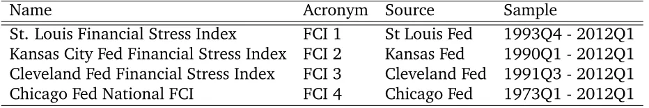
Table 1. Financial Conditions and Stress indices

Name Acronym Source Sample

St. Louis Financial Stress Index FCI 1 St Louis Fed 1993Q4 - 2012Q1 Kansas City Fed Financial Stress Index FCI 2 Kansas Fed 1990Q1 - 2012Q1 Cleveland Fed Financial Stress Index FCI 3 Cleveland Fed 1991Q3 - 2012Q1

Chicago Fed National FCI FCI 4 Chicago Fed 1973Q1 - 2012Q1

3.2 Choice of hyperparameters and initial conditions

In this section we outline the setting of various hyperparameters and initial conditions. All our benchmark choices that apply in the next two subsections are fairly non-informative. In Appendix C we implement a sensitivity analysis using priors based on a training data sample, thus extending the recommendations of Primiceri (2005) to our TVP-FAVARs.

The first step is to set the initial conditions for the factor ft (FCI), the

time-varying parameters t; t, the time-varying covariancesVt; Qt, and, for doing DMA

and DMS, we must specify 0j0;j,j = 1; :::; J. These initial conditions are set to the

following (relatively non-informative) values

f0 N(0;4);

0 N 0;4 In(s+1) ; 0 N(0; VM IN)

V0 1 In;

Q0 1 Is+1; 0j0;j =

1

(13)

where VM IN is a diagonal covariance matrix which, following the Minnesota prior

tradition, penalizes more distant lags and is of the form

VM IN =

4; for intercepts

0:1=r2; for coefficient on lagr ; (6) where r = 1; ::; p denotes the lag number. Note that estimates of Wt and Rt are

proportional to the respective state covariance matrices obtained from the Kalman filter, therefore there is no need to initialize these matrices; see the Technical Appendix for more details.

Regarding the decay and forgetting factors we have introduced in our model it is worth noting that we can estimate these from the data. However, computation increases substantially (we need to evaluate or maximize the predictive likelihood for each combination of the various factors) and, as shown in Koop and Korobilis (2013), the existence of value added in forecasting performance from such a procedure is questionable. Given these considerations, we choose to fix the values of the decay/forgetting factors, but investigate sensitivity to their choice in Appendix C.

For the decay factors 1; 2 which control the variation in the covariance matrices, we fix these to the value 0:96. Such values provide volatility estimates which are quite close to the ones expected by integrated stochastic volatility models that have been used extensively in the Bayesian VAR and FAVAR literature (Primiceri, 2005; Korobilis, 2013). For the forgetting factors 3; 4, we follow the “business as usual prior” approach of Cogley and Sargent (2005) and assume that changes each period are relatively slow and stable under the random walk specification in equation (2). In order to achieve this slow time variation in the coefficients, we set 3 = 4 = 0:99, a setting we use in all TVP-FAVAR and TVP-VAR specifications. As described in the Technical Appendix, restricted versions of our general model can be obtained by setting the forgetting factors to one. For instance when 3 = 4 = 1, we obtain the VAR model.

Finally, we need to choose our prior beliefs about model change. The value of the forgetting factor determines how fast model switches occur, and thus we use two values: = 1 which implies that we are implementing Bayesian model averaging (BMA) given data up to time t; and = 0:99 which implies that we implement dynamic model averaging (DMA) with relatively slowly varying model probabilities.

3.3 Estimates of the Financial Conditions Index

(14)

Figure 1 shows the FCI estimated in various ways using all 18 financial variables without any model selection or model averaging being done. The shaded regions in this figure (and subsequent figures) are the NBER recession dates. The estimated FCIs are all similar to each other. In particular, the TVP-FAVAR and principle components are producing very similar FCIs. The FCI produced by the FAVAR does differ from the others at some points, particularly in the first half of the sample. This indicates the potential importance of allowing for time variation in parameters. It is interesting to note that the FCIs start declining before the beginning of the recent recession with all of them bottoming out in early 2009. However, after 2009 some discrepancies appear between the FCIs.

Figure 2 shows the impact of model averaging and selection on the estimate of the FCI, focussing on the TVP-FAVARs. Although the broad patterns in the FCIs plotted in Figure 2 are similar, there are some differences. In general, the FCIs in Figure 2 are less smooth than in Figure 1 indicating that model switching/averaging is reacting more quickly than methods without such a feature. And there are some interesting small divergences between the two figures. For instance, in Figure 2 there is a slight improvement in the FCIs early on in the recent recession which is missing from Figure 1. DMA and DMS are producing factor estimates which are very similar to one another.

In Figure 3 we perform a comparison of the FCI constructed using DMA on the TVP-FAVAR models with the four FCIs or FSIs maintained by four Federal Reserve Banks (see Table 1). As discussed previously, FCIs and FSIs are somewhat different since FSIs are measuring financial stress (and, hence, it is the comparison of our approach with the Chicago Fed’s National Financial Conditions Index which is the most relevant). We have multiplied the FSIs by minus one to maintain comparability with the FCIs. Additionally, we standardize all the indices to have mean zero and variance one. Our FCI does indeed match up most closely with the Chicago Fed’s FCI. Our FCI started dropping earlier than the Chicago Fed’s in 2008 and dropped to a lower value at the depth of the current recession. In contrast, after the 2001 recession ended, our FCI grew faster and peaked at a higher level than the Chicago Fed’s. However, there are substantive differences with the FSIs. It is interesting to note that, after this 2001 recession ended, the FSIs continued to signal deteriorating financial conditions for much longer than our FCI. In general, the FSIs (in particular, the Cleveland Fed’s FCI) exhibit substantively different behavior from our FCI.

(15)

[image:15.595.102.503.107.321.2]

Figure 1. FCIs constructed from several versions of the heteroskedastic factor-augmented VAR model with all 18 financial variables used (no model averaging/selection). For comparison, the principal component of the 18 financial

variables is also plotted.

[image:15.595.102.495.402.653.2]

(16)

[image:16.595.100.504.107.319.2]

Figure 3. The FCI from the TVP-FAVAR with DMA compared to existing financial indexes maintained by four regional US central banks.

To provide some additional insight on what DMA is doing, we present Figures 4 and 5 which shed light on the number of variables selected when we do DMA or DMS on the TVP-FAVARs. In particular, Figure 4 calculates the expected number of variables used to extract the FCI at each point in time. If we denote by nj the

number of variables which load on the FCI under modelMj, then we calculate each

time period the following expectation9

E nDM A_t =

J

X

j=1

tjt;j nj

!

1:

Figure 4 shows DMA or DMS is achieving a strong degree of parsimony. Given 17 variables to choose between, it is tending to choose between 5 and 8. There is a slow decrease in the number of variables chosen until the late 90s, then there was an abrupt increase until the current recession. Interestingly, in the middle of the recent recession, the number of variables selected started dropping again before stabilizing at the end of the recession.

(17)

[image:17.595.101.504.107.318.2]

Figure 4. Average number of variables used to extract the FCI at each point in time as implied by DMA applied in the full TVP-FAVAR specification.

(18)

1982Q1 1994Q1 2006Q1 0

0.5 1

Probability of TWEXMMTH

1982Q1 1994Q1 2006Q1 0

0.5 1

Probability of OILPRICE

1982Q1 1994Q1 2006Q1 0

0.5 1

Probability of TED spread

1982Q1 1994Q1 2006Q1 0

0.5 1

Probability of 10/2 y spread

1982Q1 1994Q1 2006Q1 0

0.5 1

Probability of 2y/3m spread

1982Q1 1994Q1 2006Q1 0

0.5 1

Probability of Commercial Paper spread

1982Q1 1994Q1 2006Q1 0

0.5 1

Probability of LOANHPI Index

1982Q1 1994Q1 2006Q1 0

0.5 1

Probability of 30y Mortgage Spread

1982Q1 1994Q1 2006Q1 0

0.5 1

Probability of CMDEBT

1982Q1 1994Q1 2006Q1 0

0.5 1

Probability of CCI Index

1982Q1 1994Q1 2006Q1 0

0.5 1

Probability of MOVE Index

1982Q1 1994Q1 2006Q1 0

0.5 1

Probability of VIX

1982Q1 1994Q1 2006Q1 0

0.5 1

Probability of TOTALSL

1982Q1 1994Q1 2006Q1 0

0.5 1

Probability of STDSCOM

1982Q1 1994Q1 2006Q1 0

0.5 1

Probability of MICH1

1982Q1 1994Q1 2006Q1 0

0.5 1

Probability of MICH2

1982Q1 1994Q1 2006Q1 0

0.5 1

Probability of MICH3 1982Q1 1994Q1 2006Q1

0 0.5 1

[image:18.595.102.490.108.378.2]

Probability of S&P500

Figure 5. Time-varying probabilities of inclusion to the final FCI for each of the 18 financial variables (S&P500 is always included; see Section 3.1). Zero probabilities

at the beginning of the sample for some of the variables correspond to periods of missing observations.

3.4 Forecasting

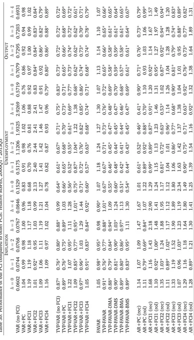
In this section, we investigate the performance of a wide range of models and methods for forecasting inflation, output growth and the unemployment rate. Our forecast evaluation period is 1990Q1 through 2013Q3-hforh= 0;1;2;3;4quarters ahead. Note that, since we are using real-time data, it is also informative to present nowcasts and these are labelled h = 0 in the tables.10 _{Evaluation of forecast} accuracy is based on the mean squared forecast error (MSFE) and average of predictive likelihoods (APL). The former evaluates the quality of point forecasts whereas the latter evaluates the quality of the entire predictive distribution. Results are normalized by dividing an MSFE or APL by the corresponding value produced by a benchmark model. We use a homoskedastic VAR (with no FCI) as our

10_{To be precise, at time} _t _{(given delays in release of macroeconomic variables) we have}

(19)

benchmark.11 _{For this benchmark model, the table presents the actual value of} MSFE or APL. Details of our choices of forgetting and decay factors are given in Section 2 and we investigate the sensitivity of results to their choice in Appendix C. The notation in the table (and the tables in Appendix C) extends our previous notation. Thus, TVP-FAVAR indicates the TVP-FAVAR with all 18 financial variables whereas TVP-FAVAR-DMA uses DMA (with = 0:99) over the 217 _TVP-FAVARs. Notation such as TVP-FAVAR (c1, c2) means that we set 1 = 2 = c1 and 3 = 4 = c2. We also present results for a VAR containing the macroeconomic variables plus a factor estimated using principle components (labelled VAR+PC). As another simple comparator, we also produce OLS (diffuse prior Bayesian) forecasts from AR models augmented with a factor (estimated by principal components). At each point in time, we choose the lag length which has produced the lowest MSFE over the last 40 quarters. From this model, we present recursive (labelled AR+PC(rec)) and rolling (labelled AR+PC(rol)) forecasts. For the rolling forecasts, we try windows of 25, 30, 35 and 40 periods and present results for the one which produces the lowest MSFE over the last 40 quarters.

For the MSFE’s we also present the Bayesian variant of a test of forecast accuracy developed in Diebold and Mariano (1995). This test is described in Appendix B of Garratt et al (2009). If an MSFE in the table has a *, it means the approach forecasts significantly differently from the benchmark VAR.

Table 2 is organized so that each panel begins with a standard benchmark (e.g. the homoskedastic VAR), then adds heteroskedasticity (e.g. the TVP-VAR(0:96, 1) which selects the forgetting factor so as to make the VAR coefficients constant over time but allows for heteroskedasticity), then adds time variation in coefficients (e.g. the TVP-VAR(0:96, 0:99)). Then the next panel in the table repeats the process with models which include FCIs beginning with the FAVAR. The subsequent panel investigates the usefulness of DMA or DMS.

In general, Table 2 shows a pattern where forecasts improve as we add in extensions. Adding heteroskedasticity tends to improve forecasts substantially, then adding time-variation in parameters tends to improve them a bit more. Moving from TVP-VARs to TVP-FAVARs leads to further improvements in forecast performance. Using DMA or DMS with the 217 _{TVP-FAVARs leads to yet further} improvements. Of course, there are some exceptions to this pattern. Table 2 investigates forecasting performance for three variables at five different horizons using two different forecast evaluation metrics. With so many possible forecast evaluations it is not surprising there are some cases where simpler approaches beat our more complicated TVP-FAVAR-DMS or TVP-FAVAR-DMA approaches. But overall the latter are tending to produce the best forecasts.

Another important pattern in Table 2 is that our approach (again with some

11_{This VAR is obtained as the restricted special case of the TVP-FAVAR (i.e. dropping the equation}

(20)

(21)

[image:21.595.93.545.105.686.2]

Table 2: Performance of our FCI compared to other forecasting models, 1990Q1 - 2013Q3

Forecast Metric APL MSFE

INFLATION

h= 0 h= 1 h= 2 h= 3 h= 4 h= 0 h= 1 h= 2 h= 3 h= 4

VAR (no FCI) 0.8587 0.7470 0.6959 0.6319 0.5848 0.0440 0.0540 0.0570 0.0610 0.0730 TVP-VAR (0.96,1) 1.36 1.31 1.32 1.32 1.29 1.05* 0.92* 0.92* 0.95* 0.97* TVP-VAR (0.96,0.99) 1.35 1.32 1.33 1.32 1.28 0.93* 0.84* 0.87* 0.93* 0.96*

FAVAR 1.00 1.00 0.99 1.02 1.01 0.96 0.90 0.86* 0.89* 0.86

TVP-FAVAR (0.96,1) 1.36 1.32 1.33 1.32 1.32 1.08* 0.94* 0.92* 0.92* 0.93* TVP-FAVAR (0.96,0.99) 1.34 1.34 1.35 1.34 1.31 0.91* 0.78* 0.78* 0.87* 0.92*

TVP-FAVAR-DMA (0.96,0.99) 1.47 1.46 1.48 1.50 1.47 0.94* 0.78* 0.82* 0.90* 0.91* TVP-FAVAR-DMS (0.96,0.99) 1.50 1.48 1.50 1.53 1.49 1.02* 0.86* 0.94* 1.07* 1.08* TVP-FAVAR-BMA (0.96,0.99) 1.35 1.36 1.38 1.38 1.32 0.94* 0.79* 0.83* 0.91* 0.92* TVP-FAVAR-BMS (0.96,0.99) 1.42 1.42 1.44 1.45 1.42 1.01* 0.84* 0.93* 1.06* 1.06*

VAR+PC 0.99 1.00 1.00 1.02 1.03 0.96 0.91 0.92 0.94* 0.90*

AR + PC (rec) 1.02 1.09 1.06 1.05 1.04 1.41* 1.39* 1.61* 2.09* 2.28* AR + PC (rol) 1.36 1.58 1.62 1.58 1.59 1.17* 0.90* 0.93* 1.12* 1.21*

UNEMPLOYMENT

h= 0 h= 1 h= 2 h= 3 h= 4 h= 0 h= 1 h= 2 h= 3 h= 4

FAVAR 0.91 0.87 0.83 0.82 0.81 0.99 1.14 1.25 1.29 1.34

VAR+PC 0.94 0.92 0.91 0.90 0.88 0.93 0.99 1.08 1.13 1.17

AR + PC (rec) 0.97 1.14 1.22 1.28 1.38 1.27 0.79* 0.64* 0.54* 0.47* AR + PC (rol) 1.12 1.30 1.34 1.34 1.41 1.11 0.76* 0.74* 0.70* 0.55*

OUTPUT

h= 0 h= 1 h= 2 h= 3 h= 4 h= 0 h= 1 h= 2 h= 3 h= 4

FAVAR 0.97 0.97 0.97 0.97 0.98 0.92 1.00 0.95 0.87 0.83

VAR+PC 1.03 1.01 1.00 0.99 0.99 0.80* 0.93* 0.96* 0.94* 0.94*

AR + PC (rec) 1.10 1.14 1.16 1.17 1.17 0.97* 0.78* 0.83* 0.79* 0.85* AR + PC (rol) 1.29 1.27 1.26 1.29 1.35 1.04* 0.90* 0.98* 1.00* 0.93*

Notes: APL is the average predictive likelihood (not in logarithms), and MSFE is the mean squared forecast error. Model’s fore-cast performance is better when APL (MSFE) is higher (lower). For each variable (inflation, unemployment, output) the first

li-ne shows the APL and MSFE of the benchmark model for each forecast horizonh. All other models’ APL and MSFE are relative

(22)

Also of interest is the performance of our approach relative to VAR forecasts augmented with an existing FCI. Before doing so, we note that such comparisons are extremely difficult since different indices are based on different assumptions, data transformations, frequencies and sample sizes. The earliest common starting date for the FCIs is 1994Q1 and, accordingly, we re-estimate our models using data from this point and use 2000Q1 - 2013Q3-h as our forecast evaluation period. Table 1 describes the existing FCIs and FSIs and defines the acronyms we use in Table 3. We use the same naming convention as in Table 2 so that, for instance, TVP-VAR+FCI4 is the TVP-VAR which includes the macroeconomic variables and the Chicago Fed National FCI. All modelling choices (e.g. priors and discount factors) are the same benchmark choices as those used previously (see Section 3.2).

In relation to the approach developed in this paper, the story is similar to that told by Table 2. TVP-FAVARs with DMA or DMS still are either the best or among the best forecasting models for all the macroeconomic variables at all forecasting horizons. The table also shows that substantial benefits can be achieved by allowing for time-variation in parameters and doing DMA or DMS. Among the existing FCIs, use of the Chicago Fed’s National FCI tends to lead to the best forecasting performance. Given the fact that it is this FCI which is most similar to our own (see Figure 3), it is not surprising that the TVP-VAR which includes FCI4 is given forecasting results similar to our TVP-FAVAR which includes all of the financial variables. Nevertheless, it is worth noting that DMA or DMS do add additional improvements in forecast performance so that DMA and TVP-FAVAR-DMS almost always forecast better than the TVP-VAR-FCI4.

(23)

[image:23.595.101.488.36.717.2]

(24)

[image:24.595.100.489.36.716.2]

(25)

4 Conclusions

In this paper, we have argued for the desirability of constructing a dynamic financial conditions index which takes into account changes in the financial sector, its interaction with the macroeconomy and data availability. In particular, we want a methodology which can choose different financial variables at different points in time and weight them differently. We develop DMS and DMA methods, adapted from Raftery et al (2010) and others, to achieve this aim. Using a large data set of US macroeconomic and financial variables, we find our estimated FCI to have reasonable properties. It is broadly similar to existing FCIs, but does exhibit some interesting differences.

(26)

References

[1] Aiolfi, M., Capistrán, C., Timmermann, A., 2010. Forecast combinations. In: Michael P. Clements and David F. Hendry (Eds). The Oxford Handbook of Economic Forecasting. Oxford University Press, USA.

[2] Balakrishnan, R., Danninger, S., Elekdag, S., Tytell, I., 2009. The transmission of financial stress from advanced to emerging economies. IMF Working Papers 09/133, International Monetary Fund.

[3] Banerjee, A., Marcellino, M., Masten, I., 2008. Forecasting macroeconomic variables using diffusion indexes in short samples with structural change. CEPR Discussion Papers 6706, C.E.P.R. Discussion Papers.

[4] Bates, B. J., Plagborg-Møller, M., Stock, J. H., Watson, M. W., 2013. Consistent factor estimation in dynamic factor models with structural instability. Journal of Econometrics, 177, 289-304.

[5] Beaton, K., Lalonde, R., Luu, C., 2009. A financial conditions index for the United States. Bank of Canada Discussion Paper, November.

[6] Bernanke, B., Boivin, J., Eliasz, P., 2005. Measuring monetary policy: A factor augmented vector autoregressive (FAVAR) approach. Quarterly Journal of Economics 120, 387-422.

[7] Boivin, J., Ng, S., 2006. Are more data always better for factor analysis? Journal of Econometrics 132, 169-194.

[8] Brave, S., Butters, R., 2011. Monitoring financial stability: a financial conditions index approach. Economic Perspectives, Issue Q1, Federal Reserve Bank of Chicago, 22-43.

[9] Breitung, J., Eickmeier, S., 2011. Testing for structural breaks in dynamic factor models. Journal of Econometrics, 163(1), 71-84.

[10] Clark, T., 2009. Real-time density forecasts from VARs with stochastic volatil-ity. Federal Reserve Bank of Kansas City Research Working Paper 09-08.

[11] Cogley, T., Sargent, T. J., 2005. Drift and volatilities: Monetary policies and outcomes in the post WWII U.S. Review of Economic Dynamics 8(2), 262-302.

[12] D’Agostino, A., Gambetti, L., Giannone, D. (2013). Macroeconomic forecast-ing and structural change. Journal of Applied Econometrics, 28, 81-101.

(27)

[14] Diebold, F., Mariano, R., 1995. Comparing predictive accuracy. Journal of Business Economics and Statistics, 13, 134-144.

[15] Doz, C., Giannone, D., Reichlin, L., 2011. A two-step estimator for large approximate dynamic factor models based on Kalman filtering. Journal of Econometrics 164, 188-205.

[16] Eickmeier, S., Lemke, W., Marcellino, M., 2011a. Classical time-varying FAVAR models - estimation, forecasting and structural analysis. Deutsche Bundesbank, Discussion Paper Series 1: Economic Studies, No 04/2011.

[17] Eickmeier, S., Lemke, W., Marcellino, M., 2011b. The changing international transmission of financial shocks: evidence from a classical time-varying FAVAR. Deutsche Bundesbank, Discussion Paper Series 1: Economic Studies, No 05/2011.

[18] English, W., Tsatsaronis, K., Zoli, E., 2005. Assessing the predictive power of measures of financial conditions for macroeconomic variables. Bank for International Settlements Papers No. 22, 228-252.

[19] Filippeli, T. and Theodoridis, K., 2013. DSGE priors for BVAR models, Empirical Economics, forthcoming.

[20] Forni M., Hallin M., Lippi M., Reichlin L., 2003. Do financial variables help forecasting inflation and real activity in the EURO area? Journal of Monetary Economics 50, 1243-55.

[21] Garratt, A., Koop, G., Mise, E. and Vahey, S., 2009. Real-time prediction with UK monetary aggregates in the presence of model uncertainty. Journal of Business and Economic Statistics, 27, 480-491.

[22] Giannone, D., Reichlin, L., Sala, L., 2005. Monetary Policy in Real Time. NBER Chapters, in: NBER Macroeconomics Annual 2004, Volume 19, pages 161-224, National Bureau of Economic Research, Inc.

[23] Gomez, E., Murcia, A., Zamudio, N., 2011. Financial conditions index: Early and leading indicator for Colombia? Financial Stability Report, Central Bank of Colombia.

[24] Hatzius, J., Hooper, P., Mishkin, F., Schoenholtz, K., Watson, M., 2010. Financial conditions indexes: A fresh look after the financial crisis. NBER Working Papers 16150, National Bureau of Economic Research, Inc.

(28)

[26] Ingram, B., Whiteman, C., 1994. Supplanting the ’Minnesota’ prior: Forecast-ing macroeconomic time series usForecast-ing real business cycle model priors. Journal of Monetary Economics, 34, 497-510.,

[27] Kárný, M., 2006. Optimized Bayesian Dynamic Advising: Theory and Algo-rithms, Springer-Verlag New York Inc.

[28] Kaufmann, S., Schumacher, C., 2012. Finding relevant variables in sparse Bayesian factor models: Economic applications and simulation results. Deutsche Bundesbank Discussion Paper No 29/2012.

[29] Koop, G., Korobilis, D., 2012. Forecasting inflation using dynamic model averaging. International Economic Review 53, 867-886.

[30] Koop, G., Korobilis, D., 2013. Large time-varying parameter VARs. Journal of Econometrics, 177, 185-198.

[31] Korobilis, D., 2013. Assessing the transmission of monetary policy shocks using time-varying parameter dynamic factor models. Oxford Bulletin of Economics and Statistics 75, 157-179.

[32] Kulhavý, R., Kraus, F., 1996. On duality of regularized exponential and linear forgetting. Automatica 32,1403-1416.

[33] Lo Duca, M., Peltonen, T., 2013. Assessing systemic risks and predicting systemic events. Journal of Banking and Finance 37, 2183-2195.

[34] Lütkepohl, H., 2005. New Introduction to Multiple Time Series Analysis. Springer: New York.

[35] Matheson, T., 2011. Financial conditions indexes for the United States and Euro Area. IMF Working Papers 11/93, International Monetary Fund.

[36] Nelson, L., Stear, E., 1976. The simultaneous on-line estimation of parameters and states in linear systems. IEEE Transactions on Automatic Control 21, 94 -98.

[37] Primiceri. G., 2005. Time varying structural vector autoregressions and monetary policy. Review of Economic Studies 72, 821-852.

[38] Quintana, J.M., West, M., 1988. Time Series Analysis of Compositional Data. In Bayesian Statistics 3, (eds: J.M. Bernardo, M.H. De Groot, D.V. Lindley and A.F.M. Smith), Oxford University Press.

(29)

[40] Schorfheide, F., Wolpin, K. E., 2012. On the use of holdout samples for model selection. American Economic Review - Papers and Proceedings 102(3), 477-481.

[41] Stock, J. H., Watson, M. W., 2002. Macroeconomic forecasting using diffusion indexes. Journal of Business & Economic Statistics 20,147-162.

(30)

[image:30.595.297.496.76.716.2]

(31)

B. Technical Appendix

In this appendix, we describe the econometric methods we use to estimate a TVP-FAVAR and restricted versions of it.

We write the TVP-FAVAR compactly as

xt = zt t+ut; ut N(0; Vt) (B.1)

zt = zt 1 t+"t; "t N(0; Qt) (B.2)

t = t 1+vt; vt N(0; Wt) (B.3)

t = t 1+ t; t N(0; Rt) (B.4)

where t = ( y t)0;

f t

0 0

and zt =

yt

ft

. We also use notation wherefet is the

standard principal components estimate of ft based on xt (using data up to time

t) and _ezt =

yt

e

ft

. Additionally, if at is a vector then ai;t is the ith element of

that vector; and ifAtis a matrixAii;tis its(i; i)thelement. Estimates of time varying

parameters or latent states can be made using data available at timet 1(filtering), or timet(updating) or timeT (smoothing). We use subscript notation for this such that atj is an estimate (or posterior moment) of time-varying parameter at using

data available through period .

Our estimation algorithm requires initialization of all state variables. In partic-ular we define the following initial conditions for all system unknown parameters

f0 N 0;

f

0j0 ; (B.5)

0 N 0; 0j0 ; (B.6)

0 N 0; 0j0 ; (B.7)

V0 1 In; (B.8)

Q0 1 Is+1: (B.9)

The algorithm follows the following steps:

1. Given the initial conditions andzt=eztobtainfilteredestimates of t; t; Vt; Qt

using the following recursion for t= 1; ::; T (a) The Kalman filter tells us:

tjData1:t 1 N tjt 1; tjt 1 ;

(32)

where tjt 1 = t 1jt 1, tjt 1 = t 1jt 1 + cWt, tjt 1 = t 1jt 1 and

tjt 1 = t 1jt 1 + Rbt. The error covariances are estimated using forgetting factors as:Wct= 1 31 t 1jt 1andRbt = 1

1

4 t 1jt 1. (b) Calculate estimates of Vt and Qt for use in the updating step using the

following EWMA specifications:

b

Vi;t = 1Vi;t 1jt 1+ (1 1)ubi;tbu0i;t (B.10)

b

Qt = 2Qt 1jt 1+ (1 2)b"tb"0t (B.11)

whereu_bi;t =xi;t zet i;tjt 1, fori= 1; :::; n, andb"t =zet ezt 1 tjt 1. (c) Update t and t given information at time t using the Kalman filter

update step

Update i;t for each i= 1; :::; nusing

itjData1:t N i;tjt; ii;tjt ;

where i;tjt = i;tjt 1 + ii;tjt 1ze0t Vbii;t+ezt ii;tjt 1ezt0

1

xt ezt tjt 1 and _ii;t_j_t= _ii;t_j_t ₁ _ii;t_j_t ₁_ez0

t Vbii;t+zet _ii;t_j_t ₁ze0t

1

e

zt _ii;t_j_t ₁:

Update _tfrom

tjData1:t N tjt; tjt ;

where _t_j_t= _t_j_t ₁+ _t_j_t ₁z_e0

t 1 Qbt+ezt 1 _t_j_t ₁ezt0 1 1

e

zt zet 1btjt 1 and _t_j_t= _t_j_t ₁ _t_j_t ₁z_e0

t 1 Qbt+ezt 1 _t_j_t ₁ezt0 1 1

e

zt 1 _t_j_t ₁: (d) UpdateVt andQt given information at timetusing the EWMA

specifica-tions as follows:

Vi;tjt = 1Vi;t 1jt 1+ (1 1)ubi;tjtbu0i;tjt (B.12)

Qtjt = 2Qt 1jt 1+ (1 2)b"tjtb"0tjt (B.13)

whereu_bi;tjt=xi;t zet i;tjt, fori= 1; :::; n, andb"tjt =zet ezt 1 tjt.

2. Obtainsmoothed estimates of t; t; Vt; Qtusing the following recursions for

t=T 1; ::;1

(a) Update t and t given information at timet+ 1using the fixed interval

(33)

Update i;t for each i= 1; :::; nfrom

itjData1:T N i;tjT; ii;tjT ;

where i;tjT = i;tjt+Ct i;t+1jT i;t+1jt , ii;tjT = ii;tjt+Ct ii;t+1jT ii;t+1jt Ct0

andC_t = _ii;t_j_t _ii;t₊₁_j_t 1: Update _tfrom

tjData1:T N tjT; tjT ;

where _t_j_T = _t_j_t+C_t _t₊₁_j_T _t₊₁_j_t , _t_j_T = _t_j_t+C_t _t₊₁_j_T _t₊₁_j_t C_t0 andC_t = _t_j_t _t₊₁_j_t 1:

(b) Update Vt and Qt given information at time t + 1 using the following

equations

V_t_j_t₊₁1 = 1V_t_j_t1+ (1 1)V_t₊₁1_j_t₊₁; (B.14) Q_t_j_t1₊₁ = 2Q_t_j_t1+ (1 2)Q_t₊₁1_j_t₊₁: (B.15)

3. Means and variances of ft given appropriate estimates of t; t; Vt; Qt

de-scribed in the preceding steps can be obtained using the standard Kalman filter and smoother.

Treatment of missing values

In our application our sample is unbalanced, since it contains many financial variables which have been collected only after the 1970s or the 1980s. Similar issues are faced by organizations which monitor FCIs. For instance, the Chicago Fed National FCI comprises 100 series where most of them have different starting dates. Although specific computational methods for dealing with such issues exist (e.g. the EM algorithm or Gibbs sampler with data augmentation), our focus is on averaging over many models which means such methods are computationally infeasible. Accordingly, similar to our purpose of developing a simulation-free and fast algorithm for parameter estimation, we want to avoid simulation methods for estimating the missing data in xt. Additionally, methods such as interpolation can

work poorly when missing values are at the beginning of the sample.

Since the missing data in xt are in the beginning, we make the assumption

that the factor (FCI) is estimated using only the observed series. The estimation algorithm above allows for such an approach in a straightforward manner by just replacing missing values with zeros. The loadings (whether time-varying, or constant) will become equal to 0, thus removing from the estimate of ft the effect

(34)

for the initial principal components estimate fet, as well as the final Kalman filter

estimate.

Estimation of a single TVP-FAVAR

Given the algorithm above, we can estimate the TVP-FAVAR by choosing values of 1; 2; 3; 4 < 1. For the main results in the paper we set 1 = 2 = 0:96 and 1 = 2 = 0:99. The restricted special cases of the TVP-FAVAR listed in Section 2.1 can be obtained by setting forgetting and/or decay factors to particular values. If we set 3 = 1 and 4 < 1 then we can obtain a TVP-VAR augmented with factors estimated with constant loadings12_{. Setting}

3 = 1 and 4 = 1leads to the constant parameter FAVAR with heteroskedastic covariances (assuming that 1; 2 <1). If we additionally set 1 = 2 = 1we can estimate homoskedastic versions of the various models, since in that caseVt =Vt 1 =:::=V1 =V0 and Qt =Qt 1 =:::=Q1 =Q0. Nevertheless, as discussed in the main body of the paper, this is a case which is always dominated (in terms of forecast performance) by the heteroskedastic case. We provide more evidence for this in Appendix C.

Estimation of multiple models (DMA/DMS)

In order to implement the DMA/DMS exercises we run the algorithm described above for each of the 217 _{= 131}_;₀₇₂ _{models. Note that for a specific DMA exercise} all models are nested, and the only thing that changes is the number of variables in the vectorxt that we use in order to extract the FCI. Given our discussion about

how missing values are treated by the Kalman filter, in order to estimate a specific model which uses, say, the 1st, 3rd and 15th series inxt, we simply multiply all but

the 1st, 3rd and 15th columns ofxtwith zeros. In that case, we remove at all times

t the effects of all 15 variables we do not use for estimation of the specific model, and at the same time we still have as a dependent variable a 18 1 dimensional vector (and programming is greatly simplified).

The most important feature of DMA is that, unlike many Bayesian model selection and averaging procedures which use MCMC methods, there is no depen-dence in estimating each model and iterations using “for” loops are independent. That means that it is trivial to adapt our code to use features such as parallel computing, thus taking advantage of the widespread availability of modern multi-core processors (or large clusters of PCs). In MATLAB this is as easy as replacing the typical “for” loop which would run for models1to131;072, with a “parfor” loop.

The reader is encouraged to look at our code which is available on https://sites.google .com/site/dimitriskorobilis/matlab, which also has the option to call the Parallel Processing Toolbox in a MATLAB environment.

12_{In a previous version of this paper we have named this model the factor augmented TVP-VAR or}

(35)

C. Sensitivity analysis

In this section we present further results for several different choices of prior hyperparameters, which can reflect different beliefs about time variation in the model parameters as well as beliefs about variation over time in the choice of the optimal model.

C.1.

Comparison of relatively noninformative with training

sample priors

In the main body of the paper results are presented for a subjectively-elicited but relatively noninformative prior. An interesting alternative is to choose all prior hyperparameters using a training sample of data. In the context of TVP-VARs, Primiceri (2005) suggests such a prior which is based on splitting the data into a training sample, and a testing sample where estimation occurs. OLS estimation of a constant coefficient model using the training sample provides parameter estimates which are used as prior hyperparameters for the testing sample. Such training sample priors are commonly-used in Bayesian analysis, and in the context of TVP models help provide regularized posterior estimators which can also help numerical stability. This latter feature is important in the case of TVP-VARs and TVP-FAVARs estimated with MCMC - see the discussion in Section 4.1 of Primiceri (2005).

In this section, we introduce such a training sample prior for our FAVAR and TVP-FAVAR models. We use the first 10 years of data (1970Q1-1979Q4) in our original sample as the training sample. We estimate a FAVAR with constant parameters using OLS methods (replacing the factor with its principal component estimate) on this training sample. These OLS estimates are used to in the initial conditions for the estimation sample, 1980Q1-2013Q3, as follows

f0 N fbTT S;0:1 ;

0 N 0;4 var b

T S

;

0 N 0;4 var b

T S

; V0 1 VbT S;

Q0 1 QbT S; 0j0;j =

1

J;

(36)

[image:36.595.91.513.265.567.2]

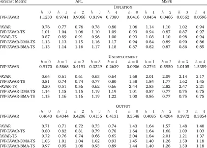
models (DMA vs BMA, or FAVAR vs TVP-FAVAR) are exactly the ones specified in Section 3.2. The forecast evaluation sample is 1990Q1-2013Q3. Table C.1 presents the results of this exercise. It is divided in three blocks, each one corresponding to one of the three variables of interest (inflation, unemployment, output growth). For each block the first line shows the APL and MSFE of the benchmark TVP-FAVAR used in the main body of the paper. The APLs and MSFEs of all other models are relative to the APL and MSFE of the benchmark TVP-FAVAR, which implies that relative APL higher than one (similarly, relative MSFE lower than one) is an indication of better performance relative to the benchmark.

Table C1: Comparison of benchmark with training sample (TS) priors, 1990Q1-2013Q3

Forecast Metric APL MSFE

INFLATION

h= 0 h= 1 h= 2 h= 3 h= 4 h= 0 h= 1 h= 2 h= 3 h= 4

TVP-FAVAR 1.1233 0.9741 0.9066 0.8194 0.7380 0.0416 0.0454 0.0466 0.0562 0.0696

FAVAR 0.76 0.77 0.76 0.78 0.80 1.06 1.14 1.10 1.02 0.94

TVP-FAVAR-TS 1.01 1.04 1.06 1.10 1.09 0.93 0.94 0.87 0.87 0.97 FAVAR-TS 0.87 0.89 0.91 0.96 1.00 0.93 1.08 1.10 0.98 0.94 TVP-FAVAR-DMA-TS 1.13 1.13 1.15 1.16 1.17 0.94 0.84 0.89 0.90 0.86 TVP-FAVAR-BMA-TS 1.13 1.14 1.16 1.17 1.18 0.87 0.82 0.87 0.86 0.85

UNEMPLOYMENT

h= 0 h= 1 h= 2 h= 3 h= 4 h= 0 h= 1 h= 2 h= 3 h= 4

TVP-FAVAR 0.9170 0.5868 0.4191 0.3229 0.2639 0.0906 0.2741 0.5950 1.0105 1.5359

FAVAR 0.64 0.61 0.61 0.63 0.64 1.68 2.01 2.09 2.14 2.17

OUTPUT

h= 0 h= 1 h= 2 h= 3 h= 4 h= 0 h= 1 h= 2 h= 3 h= 4

TVP-FAVAR 0.4643 0.4344 0.4206 0.4156 0.4131 0.3548 0.4085 0.4204 0.3972 0.3854

FAVAR 0.71 0.71 0.72 0.73 0.74 1.43 1.64 1.57 1.48 1.40

Notes: APL is the average predictive likelihood (not in logarithms), and MSFE is the mean squared forecast error. Model’s fore-cast performance is better when APL (MSFE) is higher (lower). For each variable (inflation, unemployment, output) the first

li-ne shows the APL and MSFE of the benchmark model for each forecast horizonh. All other models’ APL and MSFE are relative

to that of the benchmark model. Values of APL (MSFE) higher (lower) than 1 signify better performance than the benchmark.