Extreme M quantiles as risk measures: from L1 to Lp optimization

(1)

Extreme M-quantiles as risk measures: From

L

1

to

L

p

optimization

Supplementary Material

Abdelaati Daouia

p1q

, St´

ephane Girard

p2q

& Gilles Stupfler

p3q

p1q _{Toulouse School of Economics, University of Toulouse Capitole, France} p2q_{Team Mistis, Inria Grenoble Rhˆ}_{one-Alpes & LJK, Inovall´}_{ee, 655, av. de l’Europe,}

Montbonnot, 38334 Saint-Ismier cedex, France

p3q_{School of Mathematical Sciences, University of Nottingham, University Park,}

Nottingham NG7 2RD, United Kingdom

Supplement A contains the proofs of all theoretical results in the main paper. Supplement B provides additional

technical results and lemmas. Further simulation results are discussed in Supplement C. An application to medical

insurance data is given in Supplement D.

A

Main results and proofs

Proof of Proposition 1. The starting point is thatqτppqis a solution of the equation

p1τq_EppqXqp11I_tX quq τEppXqqp11ItX¡quq, (A.1)

which is equivalent to:

I1pq;pq p1τqI2pq;pq (A.2)

with I1pq;pq E

X q 1

p1 1I_tX¡qu

and I2pq;pq E

X_q 1

p1

.

We now claim that τ ÞÑqτppq is an increasing function on p0,1q, tending to 8 as τ Ò 1. If indeed τ ÞÑ qτppq

were not an increasing function, one could find 0 τ1 τ2 1 with qτ1ppq ¥qτ2ppq. But then, since the maps

q ÞÑ EppqXqp11ItX quqand q ÞÑ EppXqqp11ItX¡quq are respectively nondecreasing and nonincreasing, one

would get thanks to (A.1) that:

p1τ2qEppqτ2ppq Xq

p1_1I

tXqτ2ppquq p1τ1qEppqτ1ppq Xq

p1_1I

tXqτ1ppquq τ1EppXqτ1ppqq

p1_1I

tX¡qτ₁ppquq τ2EppXqτ2ppqq

p1_1I

tX¡qτ₂ppquq.

This is certainly a contradiction because of (A.1) again. Now, ifqτppqdid not tend to 8as τÒ1, then it would

converge to some finiteq due to the functionτ ÞÑqτppqbeing increasing. The functionsqÞÑEppqXqp11ItX quq

(2)

τ Ò1 in (A.1) withqqτppqthatEppXqqp11ItX¡quq 0. Consequently X ¤q with probability 1, which is

a contradiction sinceX has a heavy right-tail and thus an infinite right endpoint.

The idea is then to compute asymptotic equivalents of both the expectationsI1pq;pqandI2pq;pqasqÑ 8 and then solve equation (A.2) by replacing these terms by the aforementioned equivalents with qτppq substituted in

place ofq.

We start by computing an asymptotic equivalent ofI1pq;pq. Write

I1pq;pq E

H

X q

Hp1q

1I_tX¡qu

withHpxq px1qp1_1I

tx¥1u, and apply Lemma 1(i) withb1 to get

I1pq;pq Fpqq

» 8

1

pp1qpx1qp2x1{γdxp1 op1qq.

An integration by parts and the change of variablesy 1{xentail

I1pq;pq

Fpqq γ

» ₈

1

px1qp1x1{γ1dxp1 op1qq

Fpqq

γ

»1

0

p1yqp1y1{γpdyp1 op1qq

Fpqq

γ Bpp, γ

1_p ₁_qp₁ _o_p₁_qq _(A.3)

asqÑ 8.

We now examineI2pq;pq. Write

I2pq;pq I1pq;pq E

Xq 1

p11I_tX qu

E

Xq 1

p11I_t|X|¤qu

. (A.4)

By (A.3), the first term on the right-hand side above converges to 0 asqÑ 8. The second one is controlled by writing

E

X_q 1

p1

1I_tX qu

¤

2

q

p1

E

Xp11I_tX qu opqpp1qq op1q (A.5)

as q Ñ 8, while the asymptotic behavior of the third term is obtained by noting that the integrand converges almost surely to 1 and is bounded by 2p1 _{which, by the dominated convergence theorem, entails:}

E

X_q 1

p1

1I_t|X_|¤q_u

Ñ1 as qÑ 8. (A.6)

Combining (A.3), (A.4), (A.5) and (A.6), we arrive at

I2pq;pq Ñ1 as qÑ 8. (A.7)

Using (A.3) and (A.7), equation (A.2) thus yields

1τFpqτppqq

Bpp, γ1p 1q

γ p1 op1qq

(3)

Proof of Proposition 2. As in the proof of Proposition 1, the starting point is the fact thatqτppqis the unique

solution of equation (A.2). Let us provide an asymptotic expansion of both sides of this equation asτÒ1.

The left-hand side of (A.2) is the easiest part: we use Lemma 1(ii) withHpxq px1qp1_1I

tx¥1uandb1 to get, asqÑ 8,

I1pq;pq

Fpqq

Bpp, γ1

r p 1q

γr

A

1

Fpqq

» ₈

1

pp1qpx1qp2x1{γrx

ρ{γr₁

γrρ

dxp1 op1qq. (A.8)

Whenρ 0, an integration by parts and the change of variables y1{xentail

I1pq;pq

Fpqq

Bpp, γ_r1p 1q

γr

A

1

Fpqq

1

γrρ

1ρ γr

Bpp,p1ρqγ_r1p 1q 1

γr

Bpp, γ_r1p 1q

p1 op1qq (A.9)

asqÑ 8.

Let us now turn to the right-hand side of (A.2), which we break down as:

E

X_q 1

p1

I1pq;pq E

1X

q

p1 1I_tX_¤q_u

. (A.10)

An equivalent ofI1pq;pqis already known by (A.3):

I1pq;pq

Bpp, γr1p 1q

γr

Fpqqp1 op1qq

asqÑ 8. The second term in (A.10) can be decomposed itself as follows:

E

1X

q

p1 1I_tX¤qu

E

#

1X

q

p1

1

+

1I_tX¤qu

Fpqq

J1pq;pq J2pq;pq 1Fpqq (A.11)

with J1pq;pq E

#

1X

q

p1

1

+

1I_t0 X¤qu

and J2pq;pq E

#

1X

q

p1

1

+

1I_tX0_u

.

We start by examining the asymptotic behavior ofJ1pq;pq. LetHpxq pp1q1p1xqp11I_t0_¤x_¤1_u and apply Lemma 1(iii), (iv) and (v) to obtain:

J1pq;pq pp1qE

H X q

Hp0q

1I_tX_¡0_u

pp1q

$ ' ' ' ' ' ' ' ' ' & ' ' ' ' ' ' ' ' ' %

EpX1ItX_¡0_uq

q p1 op1qq

if γr 1

or γr1 andEpX q 8,

EpX1It0 X quq

q p1 op1qq if γr1 andEpX q 8,

FpqqBpp1,1γ1

r qp1 op1qq if γr¡1,

(A.12)

asqÑ 8. To controlJ2pq;pq, notice first that

J2pq;pq E

#

1X

q

p1

1

+

1I_tX0_u

E

#

1 X

q

p1

1

+

1I_tX_¡0_u

(4)

and apply Lemma 1(iii), (iv) and (v) withHpxq pp1q1p1 xqp1to get

J2pq;pq pp1qE

H X q

Hp0q

1I_tX_¡0_u

pp1q

$ ' ' ' ' ' ' ' ' ' ' ' ' & ' ' ' ' ' ' ' ' ' ' ' ' %

EpX1ItX 0uq

q p1 op1qq

if γ` 1

or γ`1 andEpXq 8

or F is light-tailed,

EpX1Itq X 0uq

q p1 op1qq if γ`1 andEpXq 8,

FpqqBpγ_`1p 1,1γ_`1qp1 op1qq if γ`¡1.

(A.13)

This is obtained by noticing that, in the case γ` 1, we have EpX1I_t0 X quq EpX1Itq X 0uq, and in the caseγ`¡1, the change of variablesux{p1 xq, or equivalentlyxu{p1uq, yields

» ₈

0

p1 xqp2x1{γ`_dx »1

0

p1uq1{γ`p_u1{γ`_du_Bp_γ1

` p 1,1γ

1

` q.

Finally, notice that the regular variation property of A (see Theorem 2.3.3 in de Haan and Ferreira, 2006) and

Proposition 1 entail

A

1

Fpqτppqq

Bpp, γ_r1p 1q

γr

ρ

A

1 1τ

p1 op1qq. (A.14)

Combining (A.2), (A.9)–(A.14) and replacingqbyqτppqshows that

Fpqτppqq

Bpp, γ1

r p 1q

γr

A

1 1τ

Kpp, γr, ρqp1 op1qq

p1τq 1Fpqτppqq pp1qrRrpqτppq, p, γrq R`pqτppq, p, γ`qs

. (A.15)

Using Corollary 1 and the regular variation of the functionsF andF (when it is heavy-tailed), we get

Rrpqτppq, p, γrq

$ ' ' ' ' ' ' ' ' ' & ' ' ' ' ' ' ' ' ' %

EpX1ItX¡0uq

qτppq

p1 op1qq if γr 1

or γr1 andEpX q 8,

EpX1It0 X qτppquq

qτppq

p1 op1qq if γr1 andEpX q 8,

FpqτppqqBpp1,1γr1qp1 op1qq if γr¡1

$ ' ' ' ' ' ' ' ' ' ' & ' ' ' ' ' ' ' ' ' ' % γr

Bpp, γr1p 1q

γr

EpX1ItX_¡0_uq

qτp1q p

1 op1qq if γr 1

or γr1 andEpX q 8,

γr

Bpp, γr1p 1q

γr

EpX1It0 X qτp1quq

qτp1q

p1 op1qq if γr1 andEpX q 8,

γr

Bpp, γr1p 1q

Fpqτp1qqBpp1,1γr1qp1 op1qq if γr¡1

γr

Bpp, γr1p 1q

minpγr,1q

(5)

and

R`pqτppq, p, γ`q

$ ' ' ' ' ' ' ' ' ' ' ' ' & ' ' ' ' ' ' ' ' ' ' ' ' %

EpX1ItX 0uq

qτppq p

1 op1qq

if γ` 1

or γ`1 andEpXq 8

EpX1Itqτppq X 0uq

qτppq p

1 op1qq if γ`1 andEpXq 8,

FpqτppqqBpγ`1p 1,1γ

1

` qp1 op1qq if γ`¡1

$ ' ' ' ' ' ' ' ' ' ' ' ' ' ' ' ' ' & ' ' ' ' ' ' ' ' ' ' ' ' ' ' ' ' ' % γr

Bpp, γr1p 1q

γr

EpX1ItX0_uq

qτp1q p

1 op1qq

if γ` 1

or γ`1 andEpXq 8

γr

Bpp, γr1p 1q

γr

EpX1Itqτp1q X 0uq

qτp1q p

1 op1qq if γ`1 andEpXq 8,

γr

Bpp, γr1p 1q

γr{γ`

Fpqτp1qqBpγ`1p 1,1γ

1

` qp1 op1qq if γ`¡1

γr

Bpp, γr1p 1q

γr{maxpγ`,1q

R`pqτp1q, p, γ`q.

Consequently, by Proposition 1,

Fpqτppqq pp1qrRrpqτppq, p, γrq R`pqτppq, p, γ`qs

γr

Bpp, γr1p 1q

p1τqp1 op1qq

pp1q

γr

Bpp, γr1p 1q

min_pγr,1q

Rrpqτp1q, p, γrq

γr

Bpp, γr1p 1q

γr{maxpγ`,1q

R`pqτp1q, p, γ`q

.

Rearranging equation (A.15) yields

Fpqτppqq

1τ

γr

Bpp, γr1p 1q

1 A

1 1τ

γr

Bpp, γr1p 1q

Kpp, γr, ρqp1 op1qq

1

1 γr

Bpp, γr1p 1q

p1τqp1 op1qq

pp1q

γr

Bpp, γr1p 1q

minpγr,1q

Rrpqτp1q, p, γrq

γr

Bpp, γr1p 1q

γr{maxpγ`,1q

R`pqτp1q, p, γ`q

.

Using a straightforward Taylor expansion of the functionxÞÑ p1 xq1in a neighborhood of 0 completes the proof.

Proof of Proposition 3. By Proposition 2 and a Taylor expansion, 1τ

Fpqτppqq

Bpp, γr1p 1q

γr

p1Rpτ, pqp1 op1qqq.

(6)

Proof of Theorem 1. Notice thatyÞÑητpy;pq{pis continuously differentiable with derivative

ϕτpy;pq |τ1I_ty¤0u||y|p1signpyq.

Use Lemma 3 to write, for anyu,

ψnpu;pq uT1,n T2,npuq T3,npuq (A.16)

with T1,n :

1

a

np1τnq n

¸

i1 1

rqτnppqsp1

ϕτnpXiqτnppq;pq,

T2,npuq :

1

rqτnppqsp n

¸

i1

»uqτnppq{ ?

np1τnq

0

rEpϕτnpXiqτnppq t;pqq EpϕτnpXiqτnppq;pqqsdt

and T3,npuq :

1

rqτnppqsp n

¸

i1

»uq_τnppq{?np1τnq

0

rSn,ipqτnppq tq Sn,ipqτnppqqsdt

whereSn,ipvq:ϕτnpXiv;pq EpϕτnpXv;pqq.

By Lemmas 8, 9 and 10, we get

ψnpu;pq d

ÝÑ uZaVpγ;pq u

2

2γ as nÑ 8

(withZ being standard Gaussian) in the sense of finite-dimensional convergence. As a function of u, this limit is

almost surely finite and defines a convex function which has a unique minimum at

uγaVpγ;pqZd N 0, γ2Vpγ;pq.

Applying the convexity lemma of Geyer (1996) completes the proof.

Proof of Theorem 2. Write

log

p

qW τ_n1ppq

qτ_n1ppq

ppγnγqlog

1τn

1τ_n1

log

p

qτnppq

log

1τ_n1

1τn

γ

qτ_n1ppq

qτnppq

.

The convergence logrp1τnq{p1τn1qs Ñ 8 yields

a

np1τnq

logrp1τnq{p1τn1qs

log

p

qτnppq

O_P 1{logrp1τnq{p1τn1qs

o_Pp1q, (A.17)

and

a

np1τnq

logrp1τnq{p1τn1qs

log

1τn1

1τn

γ

qτ_n1ppq

qτnppq

a

np1τnq

logrp1τnq{p1τn1qs

log

qτ1_nppq

qτ_n1p1q

log

qτnppq

qτnp1q

log

1τ_n1

1τn

γ

qτ1_np1q

qτnp1q

O

_a

np1τnq

logrp1τnq{p1τn1qs

rRpτn, pq |App1τnq1q| Rpτn1, pq |App1τn1q

1_q|s

O

a

np1τnq

logrp1τnq{p1τn1qs

rRpτn, pq |App1τnq1q|s

op1q. (A.18)

Convergence (A.17) is a consequence of our Theorem 1. Convergence (A.18) follows from a combination of

Proposition 3 and of Theorem 2.3.9 in de Haan and Ferreira (2006) and, in what concerns the relationship

Rpτn1, pq OpRpτn, pqq, from the regular variation of F, F, s ÞÑ Upsq q1s1p1q and |A|. Combining these

(7)

Proof of Theorem 3. We start by writing

log

r

qW τ_n1ppq

qτ_n1ppq

log

p

qW τ_n1p1q

qτ_n1p1q

log

Cppγn;pq

Cpγr;pq

log

qτ_n1ppq

Cpγr;pqqτ_n1p1q

. (A.19)

To work on the first term on the right-hand side, note that

log

p

qW_τ1

np1q

qτ1_np1q

ppγnγqlog

1τn

1τ_n1

log

p

qτnp1q

log

1τn1

1τn

γ

qτ_n1p1q

qτnp1q

.

Sinceqpτnp1q Xntnp1τnqu,n, the convergence logrp1τnq{p1τ

1

nqs Ñ 8and a use of Theorem 2.3.9 of de Haan

and Ferreira (2006) yield:

a

np1τnq

logrp1τnq{p1τn1qs

log

p

qτnp1q

o_Pp1q,

and

a

np1τnq

logrp1τnq{p1τn1qs

log

1τ_n1

1τn

γ _q τ_n1p1q

qτnp1q

O

a

np1τnq

logrp1τnq{p1τn1qs

|App1τnq1q|

op1q.

As a consequence: _a

np1τnq

logrp1τnq{p1τn1qs

log

p

qW τ1

np1q

qτ_n1p1q

d

ÝÑζ. (A.20)

To conclude the proof, it is then enough to examine the behavior of the second and third term on the right-hand

side of Equation (A.19). First,

a

np1τnq

logrp1τnq{p1τn1qs

log

Cppγn;pq

Cpγr;pq

o_Pp1q, (A.21)

because of the anp1τnqconvergence of pγn and of the differentiability of the mapping xÞÑ logCpx;pq at γr.

Second,

a

np1τnq

logrp1τnq{p1τn1qs

log

qτ_n1ppq

Cpγr;pqqτ_n1p1q

O_P

a

np1τnq

logrp1τnq{p1τn1qs

rRpτ_n1, pq |App1τ_n1q1q|s

O_P

a

np1τnq

logrp1τnq{p1τn1qs

rRpτn, pq |App1τnq1q|s

o_Pp1q, (A.22)

which follows from a combination of Proposition 3 and of Theorem 2.3.9 in de Haan and Ferreira (2006) and, in

what concerns the relationship Rpτn1, pq OpRpτn, pqq, from the regular variation ofF,F,sÞÑUpsq q1s1p1q

and|A|. Combining these elements and using the Delta-method leads to the desired conclusion.

Proof of Theorem 4. We write

1 pτ_n1pp, αn; 1q

1τn1pp, αn; 1q

1 γr

p γn B p, 1 p γn p 1 B p, 1 γr p 1

p1αnq

1 γr B p, 1 γr p 1

1τn1pp, αn; 1q

1. (A.23)

Now

a

np1τnq

γr p γn 1 _p1 γn a

np1τnqpγr pγnq d

ÝÑ ζ

γr

(8)

by Slutsky’s lemma. Moreover, using the relationship

BB

Bypx, yq

B By

ΓpxqΓpyq

Γpx yq

Bpx, yq pΨpyq Ψpx yqq

where Ψpxq Γ1pxq{Γpxqis the digamma function, we obtain

d dx B p,1

xp 1

1

x2B

p,1

xp 1 Ψ

1

xp 1

Ψ 1 x 1 .

The delta-method then yields

a

np1τnq

B p, 1 p γn p 1 B p, 1 γr p 1 1 1 B p, 1 γr p 1 a

np1τnq

B p, 1 p γn p 1 B p, 1 γr p 1 d

ÝÑ ζ

γ2 r Ψ 1 γr p 1 Ψ 1 γr 1 . (A.25)

To complete the proof, we note that

p1αnq

1 γr B p, 1 γr p 1

1τ_n1pp, αn; 1q

p1αnq

1 γr B p, 1 γr p 1 E

_q_αX_np₁_q1

p1

1I_tX¡qαnp1qu E

qαXnp1q

1

p1

.

Recall now (A.8) in the proof of Proposition 2 which here translates into

p1αnq

_q_αX_np₁_q1

p1

1I_tX¡qαnp1qu

1

Fpqαnp1qq

_q_αX_np₁_q1

p1

1I_tX¡qαnp1qu

1

OrAp1{Fpqαnp1qqqs

OrApp1αnq1qs.

Similarly, by (A.10)–(A.13) in the proof of Proposition 2, we get

E

qαXnp1q

1

p1

1 OrmaxtFpqαnp1qq, Rrpqαnp1q, p, γrq, R`pqαnp1q, p, γ`qus

Ormaxt1αn, Rrpqαnp1q, p, γrq, R`pqαnp1q, p, γ`qus.

Combine these two asymptotic bounds to obtain

p1αnq

1 γr B p, 1 γr p 1

1τ_n1pp, αn; 1q

1Ormaxt1αn, App1αnq1q, Rrpqαnp1q, p, γrq, R`pqαnp1q, p, γ`qus. (A.26)

Combining (A.23), (A.24), (A.25) and (A.26) leads to

a

np1τnq

1 pτ_n1pp, αn; 1q

1τ_n1pp, αn; 1q

1 " 1 1 γr Ψ 1 γr p 1 Ψ 1 γr 1 * ζ γr

(9)

proving the first statement. In the case when

a

np1τnqmaxt1αn, App1αnq1q, Rrpqαnp1q, p, γrq, R`pqαnp1q, p, γ`qu Ñ0

the above equality becomes

a

np1τnq

1 pτ_n1pp, αn; 1q

1τ_n1pp, αn; 1q

1 " 1 1 γr Ψ 1 γr p 1 Ψ 1 γr 1 * ζ γr

op1q

which implies the second statement and concludes the proof.

Proof of Theorem 5. The key point is to write

p

qτ1W_p_n_pp,αn;1qppq

1 pτ_n1pp, αn; 1q

1τn

_pγn p

qτnppq

1 pτ_n1pp, αn; 1q

1τ_n1pp, αn; 1q

_pγn

#

1τ_n1pp, αn; 1q

1τn

_pγn p

qτnppq

+

. (A.27)

Now, by Theorem 4,

1 pτ_n1pp, αn; 1q

1τn1pp, αn; 1q

1 O_P

1

a

np1τnq

and therefore

1 pτ_n1pp, αn; 1q

1τ_n1pp, αn; 1q

pγn

exp

pγnlog

1 pτ_n1pp, αn; 1q

1τ_n1pp, αn; 1q

exp

γ O_P

1

a

np1τnq

O_P

1

a

np1τnq

1 O_P

1

a

np1τnq

(A.28)

by a Taylor expansion. Furthermore, we have

1τ_n1pp, αn; 1q

1τn

pγn p

qτnppq pqWτ_n1_pp,αn;1qppq

by definition of the extrapolated class of estimatorsqpW_p_p_q_{. Using the asymptotic equivalent}

1τ_n1pp, αn; 1q p1αnq

1 γr B p, 1 γr p 1 (A.29)

we conclude that the conditions of Theorem 2 are satisfied if the parameterτ_n1 there is set equal toτ_n1pp, αn; 1q. By

Theorem 2: _a

np1τnq

logrp1τnq{p1τn1pp, αn; 1qqs

p

qW τ1

npp,αn;1qppq

qτ1_n_pp,αn;1qppq 1 d ÝÑζ. Now log

1τn

1τn1pp, αn; 1q

log

1τn

1αn

log

1αn

1τn1pp, αn; 1q

and in the right-hand side of this identity, the first term tends to infinity, while the second term converges to a

finite constant in view of (A.29). As a conclusion

log

1τn

1τ_n1pp, αn; 1q

log

1τn

1αn

.

Together with the equalityqτ_n1_pp,αn;1qppq qαnp1qwhich is true by definition ofτn1pp, αn; 1q, this entails

a

np1τnq

logrp1τnq{p1αnqs

p

qW

τ1_n_pp,αn;1qppq

qαnp1q

1

d

ÝÑζ. (A.30)

(10)

Proof of Theorem 6. The proof of this result is similar to that of Theorem 5: just apply Theorem 3 instead of

Theorem 2 in order to prove the required analogue of (A.30).

Proof of Theorem 7. The proof of this result is the same as that of Theorem 3, with pq_τW1

np1qbeing replaced by p

qW_τ1

nppq[thus applying Theorem 2 to obtain an analogue of (A.20)] and the mappingxÞÑlogCpx;pqbeing replaced

byxÞÑlogrCpx; 2qC1_p_x_;_p_qs_{. The details of the proof are therefore omitted.}

Proof of Theorem 8. The proof of this result is entirely similar to that of Theorem 5 and is therefore omitted.

Proof of Theorem 9. The proof of this result is entirely similar to that of Theorem 6 and is therefore omitted.

B

Auxiliary results and proofs

Lemma 1. Let X be a random variable whose survival function F satisfies condition C1pγq, and let H be an absolutely continuous function whose derivativehis nonnegative and is such that

Da¥0, Dδ¡0, @b¡a,

» ₈

b

hpxqx1{γδdx 8.

(i) For any b¡a, we have, asqÑ 8:

E

H

X q

Hpbq

1l_tX_¡bq_u

Fpqq

» ₈

b

hpxqx1{γdxp1 op1qq.

(ii) If moreoverF satisfies conditionC2pγ, ρ, Aq, then for any b¡a, we have, asqÑ 8:

E

H

X q

Hpbq

1l_tX¡bqu

Fpqq

» ₈

b

hpxqx1{γdx A

1

Fpqq

» ₈

b

hpxqx1{γx

ρ_{γ₁

γρ dxp1 op1qq

.

Assume further that a 0 and that h is right-continuous at 0 with hp0q 1. Let X maxpX,0q denote the positive part ofX.

(iii) Ifγ 1, orγ1andEpX q 8, then, as qÑ 8:

E

H

X q

Hp0q

1l_tX¡0u

EpX q

q p1 op1qq.

This result also holds true if the functionF is actually light-tailed.

(iv) If γ1and_EpX q 8, then the function qÞÑ_EpX1l_t0Xq_uqis slowly varying and, as qÑ 8:

E

H

X q

Hp0q

1l_tX¡0u

EpX1lt0 X quq

q p1 op1qq.

(v) Ifγ¡1, then, as qÑ 8:

E

H

X q

Hp0q

1l_tX¡0u

Fpqq

» ₈

0

(11)

Proof of Lemma 1. The basic idea of the proof is to note that an integration by parts entails, forb¥a:

Ipb;qq:_E

H

X q

Hpbq

1l_tX_¡bq_u

» ₈

b

hpxqFpqxqdx.

To show (i), write

Ipb;qq Fpqq

» ₈

b

hpxqx1{γdx

» ₈

b

hpxq

Fpqxq Fpqq x

1{γ

dx

(B.1)

and use a uniform bound such as Theorem B.2.18 in de Haan and Ferreira (2006) to get

Ipb;qq Fpqq

» ₈

b

hpxqx1{γdxp1 op1qq

asqÑ 8, which is (i).

Assertion (ii) is obtained in a similar way by using (B.1), the second-order condition C2pγ, ρ, Aqand a uniform inequality such as Theorem B.3.10 in de Haan and Ferreira (2006) applied to the functionF.

The first step in order to show (iii), (iv) and (v) is to splitIp0;qqas

Ip0;qq

»ε

0

hpxqFpqxqdx

» ₈

ε

hpxqFpqxqdx

1

q

»qε

0

h

x q

Fpxqdx

» ₈

ε

hpxqFpqxqdx (B.2)

where εis an arbitrary positive real number. To prove (iii), note that if X ¤0 almost surely there is nothing to prove; otherwise, because

EpX1lt0 X qεuq

»qε

0

Fpxqdx,

we obtain:

Ip0;qq EpX1lt0 X qεuq

q

1

q

»qε

0

h

x q

1

Fpxqdx

» ₈

ε

hpxqFpqxqdx.

SinceEpX q 8the functionF is nonincreasing and integrable in a neighborhood of infinity. This entails

xFpxq ¤2

»x

x_{2

FptqdtÑ0 as xÑ 8

and therefore thatFpqq op1{qqasqÑ 8; this is of course also true ifF is light-tailed. We thus obtain, by part (i) whenF is regularly varying:

@ε¡0, Ip0;qq EpX1lt0 X qεuq

q

1

q

»qε

0

h

x q

1

Fpxqdx o

1

q

.

By the dominated convergence theorem,EpX1ltX¥qεuq Ó0 asqÑ 8and then:

@ε¡0, Ip0;qq EpX q

q

1

q

»qε

0

h

x q

1

Fpxqdx o

1

q

.

For anyα¡0, choose nowεsuch that|hpxq 1| ¤α{p1 _EpX qqfor allxP r0, εs; this yields

Ip0;qq EpX q q

¤ 1 _EαpX q

"

EpX1lt0 X qεuq

q

*

α

1 _EpX q

1

q ¤ α

q

(12)

To show (iv), use (B.2) to get for anyε¡0:

Ip0;qq 1 q »1 0 h x q

Fpxqdx

»ε

1_{q

hpxqFpqxqdx

» ₈

ε

hpxqFpqxqdx

forqlarge enough. By the right-continuity ofhat 0 and part (i) of the present Lemma, we get

Ip0;qq

»ε

1{q

hpxqFpqxqdx O

max

1

q, Fpqq

.

For an arbitraryαP p0,1q, choose nowεso small thathpxq P r1α{4,1 α{4swhenxP r0, εs. We get

1α 4

»ε

1{q

Fpqxqdx¤

»ε

1{q

hpxqFpqxqdx¤

1 α 4

»ε

1{q

Fpqxqdx

ô 1α 4

1

q

»qε

1

Fpxqdx¤

»ε

1{q

hpxqFpqxqdx¤

1 α 4 1 q »qε 1

Fpxqdx.

By Proposition 1.5.9a in Bingham et al. (1987), the functionzÞÑ³z₁Fpxqdx³z₁txFpxqudx{xis slowly varying in a neighborhood of 8(i.e. regularly varying with index 0) so that forqlarge enough,

1α 2

1

q

»q

1

Fpxqdx¤

»ε

1_{q

hpxqFpqxqdx¤

1 α 2 1 q »q 1

Fpxqdx.

Finally, we have³q₁FpxqdxÒEpX1ltX¥1uq 8 asqÑ 8and, by Proposition 1.5.9a in Binghamet al. (1987):

1

Fpqq

"

1

q

»q

1

Fpxqdx

* 1

qFpqq

»q

1

txFpxqudx x Ñ 8

asqÑ 8. In other words, forqlarge enough,

p1αq1 q

»q

1

Fpxqdx¤Ip0;qq ¤ p1 αq1 q

»q

1

Fpxqdx.

Sinceαis arbitrary, this entails

Ip0;qq 1 q

»q

1

Fpxqdxp1 op1qq 1

q

»q

0

Fpxqdxp1 op1qq EpX1lt0 X quq

q p1 op1qq

asqÑ 8: the proof of (iv) is then complete.

To show (v), letβ P p0,1qbe such that 1{γ 1β and use once again (B.2) to get:

Ip0;qq 1 q

»qβ

0 h x q

Fpxqdx

» ₈

qp1βq

hpxqFpqxqdx.

By the right-continuity ofhat 0 and the asymptotic relationshipqp1βq_o_p_F_p_q_qq_as _q_{Ñ 8}_,

Ip0;qq 1 q

»qβ

0

Fpxqdxp1 op1qq

» ₈

qp1βq

hpxqFpqxqdx

» ₈

qp1βq

hpxqFpqxqdx opFpqqq.

In the spirit of the proof of (i), write now

Ip0;qq Fpqq

» ₈

qp1βq

hpxqx1{γdx

» ₈

qp1βq

hpxq

Fpqxq Fpqq x

1{γ

dx

opFpqqq.

Since in the second integral we haveqx¥qβ _{Ñ 8}_{, we may use again a uniform bound such as Theorem B.2.18}

in de Haan and Ferreira (2006) to get

Ip0;qq Fpqq

» ₈

qp1βq

(13)

Finally, since1{γ¡ 1, the functionxÞÑx1{γ is integrable in a neighborhood of 0, and thus

Ip0;qq Fpqq

» ₈

0

hpxqx1{γdxp1 op1qq

asqÑ 8, which completes the proof of (v).

Lemma 2. Assume thatv,V are such that vpτq Ò 8andVpτq Ó0, asτÒ1, and there existsB¡0 such that

Vpτq

FpvpτqqBp1 epτqq

whereepτq Ñ0 asτÒ1. If conditionC2pγ, ρ, Aqholds, withγ¡0 andF strictly increasing, then

vpτq

Up1{Vpτqq B

γ

1 γepτqp1 op1qq Ap1{Vpτqq

Bρ1

ρ op1q

as τ Ò1.

Proof. Apply the functionU to get

vpτq

Up1{VpτqqB

γ UpBr1 epτqs{Vpτqq

Up1{Vpτqq B

γ_.

By Theorem 2.3.9 in de Haan and Ferreira (2006), we may find a functionA0, equivalent toAat infinity, such that

for anyε¡0, there ist0pεq ¡1 such that for t,tx¥t0pεq,

_A₀1_p_t_qU_Up_ptx_t_qqxγ

xγx

ρ₁

ρ

¤ _rp₂_B_qγ ρ _p_B_{₂_qγ ερ_srp₂_B_qε _p_B_{₂_qε_sx

γ ρ_max_p_xε_{, x}ε_q_.

Thus, forτ sufficiently close to 1, using this inequality witht1{VpτqandxBr1 epτqsgives that

_A₀_p₁_{1_V_p_τ_qqUpBr_U1_p₁_{e_Vpτ_pqs{_τ_qqVpτqqBγp1 epτqqγ

Bγp1 epτqqγB

ρ_p₁ _e_p_τ_qqρ₁

ρ

¤ε

and therefore

1

A0p1{Vpτqq

UpBr1 epτqs{Vpτqq Up1{Vpτqq B

γ_p₁ _e_p_τ_qqγ

ÑBγB

ρ₁

ρ as τ Ò1.

The desired result follows by a simple first-order Taylor expansion.

In the next result we use the fact thatyÞÑητpy;pq{pis continuously differentiable with derivative

ϕτpy;pq |τ1l_ty¤0u||y|p1signpyq.

Lemma 3. For allx,yP_R andτP p0,1q,

1

ppητpxy;pq ητpx;pqq yϕτpx;pq

»y

0

pϕτpxt;pq ϕτpx;pqqdt.

Proof of Lemma 3. The result follows from the identity

1

ppητpxy;pq ητpx;pqq

»xy

x

ϕτps;pqds

»y

0

ϕτpxt;pqdt

obtained by the change of variablessxt.

The next lemma gives asymptotic equivalents for a number of moments that will be used in our examination of the

(14)

Lemma 4. Assume that the survival function F satisfies condition C1pγq. Pick a ¥ 1 and assume that γ

1{rapp1qsandEpXapp1qq 8. Then:

(i) We have

Ep|ϕτpXqτppq;pq|a1l_tX¡qτppquq app1qrqτppqs

app1q_p₁_τ_qγBpapp1q, γ

1_a_p_p₁_qq

Bpp, γ1_p ₁q p1 op1qq as τ Ò1.

(ii) We have

Ep|ϕτpXqτppq;pq|a1ltX¤qτppquq p1τq

a_r_q

τppqsapp1qp1 op1qq as τÒ1.

(iii) When a¡1, we have

Ep|ϕτpXqτppq;pq|aq app1qrqτppqsapp1qp1τq

γBpapp1q, γ1_a_p_p₁_qq

Bpp, γ1_p ₁q p1 op1qq as τ Ò1.

Proof of Lemma 4. Defineθapp1q. To show (i), note that

Ep|ϕτpXqτppq;pq|a1l_tX¡qτppquq τ

a

EprXqτppqsθ1l_tX¡qτppquq

and apply Lemma 1(i) withHpxq px1qθ_1l

tx¥1u andb1 to get

EprXqτppqsθ1l_tX¡qτppquq θrqτppqs

θ_F_p_q τppqq

»₈

1

pv1qθ1v1{γdvp1 op1qq as τÒ1.

Combining this equality with Proposition 1 and the change of variablesu1v1, we obtain

EprXqτppqsθ1l_tX¡qτppquq θrqτppqs

θ_p₁_τ_q γBpθ, γ

1_θ_q

Bpp, γ1_p ₁qp1 op1qq as τÒ1 which is (i). To show (ii), write

Ep|ϕτpXqτppq;pq|a1l_tX¤qτppquq p1τq

a_r_q τppqsθE

1 X

qτppq

θ

1l_tX¤qτppqu

.

The conditions γ θ1 _and

EpXθq 8ensure that E|X|θ 8. Recall thatqτppq Ò 8 as τ Ò 1 and use the

dominated convergence theorem to get

Ep|ϕτpXqτppq;pq|a1l_tX¤qτppquq p1τq

a_r_q

τppqsθp1 op1qq

as required. Finally, combining (i) and (ii) gives (iii) and concludes the proof.

Lemma 5. Let pxnqbe a positive sequence tending to infinity and pht,nq,tPTn be a class of functions such that

sup

tPTn

sup

x_¥xn

|ht,npxq| Ñ0 as nÑ 8.

(i) Assume that the survival function F satisfies conditionH1pγq. Then:

sup

tPTn

sup

x¥xn

|ht,npxq|1

Fpxp1 ht,npxqqq

Fpxq

1ht,npxq

γ

Ñ0 as nÑ 8.

(ii) Assume that the survival functionF satisfies conditionC2pγ, ρ, Aq. Then:

sup

t_PTn

sup

x¥xn

maxp|ht,npxq|,|Ap1{Fpxqq|q

1

Fpxp1 ht,npxqqq

Fpxq

1ht,npxq

γ

(15)

Proof of Lemma 5. We first prove (i). Write for anyph, xq:

Fpxp1 hqq

Fpxq p1 hq

1{γcpxp1 hqq

cpxq exp

»x_p1 h_q

x

∆puq u du

. (B.3)

By the mean value theorem, we have fornlarge enough

|cpxp1 ht,npxqqq cpxq| ¤ |xht,npxq| max y_Prx,x_p1 ht,npxqqs

|c1pyq| ¤2|ht,npxq| max y_Prxn{2,8q

|yc1pyq|

for alltPTn andx¥xn, which entails

sup

tPTn

sup

x_¥xn

1

|ht,npxq|

|cpxp1 ht,npxqqq cpxq| Ñ0 as nÑ 8. (B.4)

Furthermore

1

|ht,npxq|

»x_p1 ht,npxqq

x

∆puq u du

¤

logp1 ht,npxqq

ht,npxq

max

y_Prx,x_p1 ht,npxqqs

|∆pyq| Ñ0

asnÑ 8 for alltPTn andx¥xn, so that the inequality|ez1| ¤ |z|e|z| yields

sup

tPTn

sup

x_¥xn

1

|ht,npxq|

exp

»xp1 ht,npxqq

x

∆puq u du

1

Ñ0 as nÑ 8. (B.5)

Combine (B.3), (B.4) and (B.5) with the Taylor expansionp1 hq1{γ 1h{γ ophqashÑ0 to complete the proof of (i).

We now turn to the proof of (ii). Using a uniform inequality such as Theorem B.3.10 in de Haan and Ferreira (2006)

applied to the functionF, we get that for any ε¡0 small enough there is x0 ¡1 such that for all x¥2x0 and

sP r1{2,2s:

1

Ap1{Fpxqq

Fpsxq Fpxq s

1{γ ¤_ε.

Applying this tos1 ht,npxq,x¥xn and lettingεÑ0 we obtain:

sup

tPTn

sup

x_¥xn

_A_p₁_{1_F_p_x_qqFpxp1 ht,npxqqq

Fpxq p1 ht,npxqq

1_{γ _o_p₁_q_.

Using again the Taylor expansionp1 hq1{γ1h{γ ophqas hÑ0 completes the proof.

The next result gives a Lipschitz property for the derivativeϕτ.

Lemma 6. For allx,hP_Randτ P p0,1q, we have

p12τqp1l_tx¤hu1ltx¤0uq|xh|p1signpxhq.

Especially,

|ϕτpxh;pq ϕτpx;pq| ¤ |h|p11lt|x|¤|h|u p1τ 1ltx¡0uq

$ ' ' ' & ' ' ' %

2|h|p1 _if ₁_p₂

(16)

Proof of Lemma 6. The equality result is a straightforward consequence of the fact that

|τ1l_tx_¤h_u| |τ1l_tx_¤0_u| p1τqp1l_tx_¤h_u1l_tx_¤0_uq τp1l_tx_¡h_u1l_tx_¡0_uq p12τqp1l_tx_¤h_u1l_tx_¤0_uq.

To show the bound on the oscillation ofϕτ, note first that

1l_tx¤hu1ltx¤0u

$ ' & ' %

1l_t0 x¤hu ifh¡0

1l_thx_¤0_u ifh 0

and consequently

|p12τqp1l_tx_¤h_u1l_tx_¤0_uq|xh|p1signpxhq| ¤

$ ' & ' %

|xh|p1_1l

t0 x¤hu ifh¡0

|xh|p1_1l

th x¤0u ifh 0

¤ |h|p11l_t|x|¤|h|u. (B.6)

Next, when 1 p 2, becausevÞÑvp2 is decreasing onp0,8qit is clear that

||xh|p1signpxhq |x|p1signpxq|

»xh

x

pp1q|v|p2dv

¤ pp1q

»_|h|

|h|

|v|p2dv

2|h|p1. (B.7)

Whenp¥2, write

||xh|p1signpxhq |x|p1signpxq|

»xh

x

pp1q|v|p2dv

¤ pp1q|h| max

vPrx,xhs|

v|p2

¤ pp1q|h|r|xh|p2 |x|p2s

by the monotonicity ofvÞÑvp2 _on_r₀_,_8q_{, and therefore}

||xh|p1signpxhq |x|p1signpxq| ¤ pp1q|h|rp|x| |h|qp2 |x|p2s

¤ pp1qp2p2 1q|h|rmaxp|x|,|h|qsp2

¤ pp1qp2p2 1qp|h|p1 |x|p2|h|q. (B.8)

Combining (B.6), (B.7) and (B.8) completes the proof.

The lemma below is a useful convergence result for the variance of row-wise partial sums of a triangular array of

strictly stationary, dependent and square-integrable random variables.

Lemma 7. Let pVi,jqbe a triangular array of square-integrable random variables such that:

• for any positive integer nand any k¤n, the random variableVn,k isσpXkqmeasurable;

(17)

Then, if the sequencepXnqisρmixing with

°₈

n1ρpnq 8, we have

lim

nÑ8

1

nVarpVn,1q Var

_n ¸

k1

Vn,k

exists and is finite.

Proof of Lemma 7. Use the strict stationarity of the sequence to obtain

Var

_n ¸

k1

Vn,k

nVarpVn,1q 2

n

¸

k2

pnk 1qCovpVn,1, Vn,kq

nVarpVn,1q

1 2

n

¸

k2

nk 1

n corrpVn,1, Vn,kq

.

It is therefore enough to show that the sequencepsnqdefined by

sn: n

¸

k2

nk 1

n corrpVn,1, Vn,kq

converges, or equivalently, that it is a Cauchy sequence. For this, we use the definition of the mixing coefficients

ρpnqto obtain, for any positive integers pandq,

|spsp q| ¤ p

¸

k2

pkp 1

p qk 1

p q

ρpk1q

p q¸

kp 1

p qk 1

p q ρpk1q

q

p q

p

¸

k2

k1

p ρpk1q

p q¸

kp 1

p qk 1

p q ρpk1q

¤ 1

p

p_¸1

k1

kρpkq

p q_¸1

kp

ρpkq.

Kronecker’s lemma gives that the first sum above is arbitrarily small forplarge enough due to the convergence of

the series°8_n₁ρpnq; besides, the second term is less than a remainder of this convergent series starting at thepth term, and is therefore arbitrarily small as well forplarge enough. Consequently|spsp q|is arbitrarily small ifp

is chosen large enough, which entails the convergence ofpsnqand concludes the proof.

The last three results are the essential steps to the proof of Theorem 1.

Lemma 8. Work under the conditions of Theorem 1. Let

T1,n

1

a

np1τnq n

¸

i1 1

rqτnppqsp1

ϕτnpXiqτnppq;pq.

Then there isσ2P r0,8q such that

T1,n d

ÝÑN 0, Vpγ;pqp1 σ2q as nÑ 8.

If moreoverpXnq is an independent sequence, thenσ20.

Proof of Lemma 8. Note that the random variablesϕτnpXiqτnppq;pq, 1¤i¤nare clearly centered because

qτnppq arg min uPR

(18)

by differentiating under the expectation sign. Write then

T1,n T1,1,n T1,2,n (B.9)

withT1,1,n

1

a

np1τnq n

¸

i1 1

rqτnppqsp1

ϕτnpXiqτnppq;pq1l_tXi¤qτnppquE ϕτnpXqτnppq;pq1ltX¤qτnppqu

andT1,2,n

1

a

np1τnq n

¸

i1 1

rqτnppqsp1

ϕτnpXiqτnppq;pq1l_tXi¡qτnppquE ϕτnpXqτnppq;pq1ltX¡qτnppqu

.

Here T1,1,n and T1,2,n are again sums of centered variables, which we analyse separately. The first term T1,1,n is

controlled by noting that sinceρpnq ¤2aφpnq(see Lemma 1.1 in Ibragimov, 1962), the series°8_n₁ρpnqconverges and we may use Lemma 7 to get

VarpT1,1,nq O

Var ϕτnpXqτnppq;pq1l_tX¤qτnppquE ϕτnpXqτnppq;pq1ltX¤qτnppqu

p1τnqrqτnppqs2pp1q

.

Using Lemma 4(ii), we conclude that VarpT1,1,nq op1τnq, proving that

T1,1,nÝÑP 0. (B.10)

We now work onT1,2,n. The essential step is to show that

T1,2,n

a

VarpT1,2,nq d

ÝÑNp0,1q. (B.11)

For this, we use the Lindeberg-type central limit theorem of Utev (1990): taking, with the notation therein,jn 1

andknn, and setting

T1,2,n n

¸

i1

Vn,i

withVn,i :

1

a

np1τnq

1

rqτnppqsp1

ϕτnpXiqτnppq;pq1l_tXi¡qτnppquE ϕτnpXqτnppq;pq1ltX¡qτnppqu

,

it is enough to show that

@ε¡0, 1

VarpT1,2,nq n

¸

i1

E

V_n,i2 1l_t|_V

n,i|¥ε ?

VarpT1,2,nqu Ñ0 as nÑ 8.

Because the Vn,i, 1 ¤ i ¤ n are identically distributed, by writing Vn,i2 V

2 δ n,i V

δ

n,i it is easy to see that this

convergence will be shown provided we prove that for some suitably smallδ¡0, the following Lyapunov condition holds:

nE|Vn,1|2 δ

rVarpT1,2,nqs1 δ{2

Ñ0 as nÑ 8. (B.12)

To prove convergence (B.12), we first obtain an equivalent of the denominator. Apply Lemma 7 to get

DcP r0,8q, lim

nÑ8

VarpT1,2,nq

nVarpVn,1q

c.

Note then that by strict stationarity,

VarpT1,2,nq

nVarpVn,1q

1 2

n

¸

k2

nk 1

(19)

It follows thatc1 in the case of independent observations; otherwise, the functionxÞÑϕτnpxqτnppq;pq1l_tx¡qτnppqu

is increasing, so that the positive quadrant dependence ofpX1, Xkqimplies that corrpVn,1, Vn,kqis nonnegative for

anykand n, see Lehmann (1966). Consequently

VarpT1,2,nq

nVarpVn,1q

1 2

n

¸

k2

nk 1

n corrpVn,1, Vn,kq ¥1.

LettingnÑ 8shows thatc¥1 and thereforec1 σ2 _{for some}_σ2_¥_{0, as required. Besides, using Lemma 4(i)} entails

nVarpVn,1q Ñ2γpp1q

Bp2p2, γ12p 2q

Bpp, γ1_p ₁q as nÑ 8. The formulasBpx, yq ΓpxqΓpyq{Γpx yqand Γpx 1q xΓpxqnow yield

2γpp1qBp2p2, γ

1₂_p ₂_q

Bpp, γ1_p ₁q Vpγ;pq so that

lim

n_Ñ8VarpT1,2,nq p1 σ

2_q _lim

n_Ñ8nVarpVn,1q Vpγ;pqp1 σ

2_q_. _(B.13)

Using this convergence, it follows that (B.12) and therefore convergence (B.11) will be shown if for some δ ¡0,

nE|Vn,1|2 δÑ0. Choose nowδ¡0 so small thatγ 1{rp2 δqpp1qsandEpXp2 δqpp1qq 8: the convergence nE|Vn,1|2 δ Ñ 0 is then a straightforward consequence of the H¨older inequality and Lemma 4(i). Hence (B.11), which recalling (B.13) is exactly

T1,2,n d

ÝÑN 0, Vpγ;pqp1 σ2q. (B.14)

Combine (B.9), (B.10) and (B.14) to conclude the proof.

Lemma 9. Work under the conditions of Theorem 1. Let

T2,npuq

n

rqτnppqsp

»uqτnppq{ ?

np1τnq

0

rEpϕτnpXqτnppq t;pqq EpϕτnpXqτnppq;pqqsdt.

Then

T2,npuq Ñ

u2

2γ as nÑ 8.

Proof of Lemma 9. By Lemma 6, we obtain

EpϕτnpXqτnppq t;pqq EpϕτnpXqτnppq;pqq

p12τnqEp|Xqτnppq t|p1signpXqτnppq tqp1l_tX¤qτnppq tu1ltX¤qτnppquqq

,

that is:

EpϕτnpXqτnppq t;pqq EpϕτnpXqτnppq;pqq

p12τnqEp|Xqτnppq t|p1signpXqτnppq tqp1l_tX_¡q_τn_pp_qu1l_tX_¡q_τn_pp_q t_uqq

τnE |Xqτnppq t|p1signpXqτnppq tq |Xqτnppq|p1signpXqτnppqq

1l_tX¡qτnppqu

p1τnqE |Xqτnppq t|

p1_sign_p_X_q

τnppq tq |Xqτnppq|p1signpXqτnppqq

1l_tX¤q_τnppqu

(20)

The idea is now to control the three terms appearing in the above representation. In all these terms, |t| varies in the intervalInpuq r0,|u|qτnppq{

a

np1τnqswhich is such that

sup

|t|PInpuq |t| qτnppq

Ñ0 as nÑ 8. (B.15)

In this proof, all opqand Opqterms are to be understood as uniform in|t| PInpuq. We also letGpxq |x|p1signpxq,

whose (Lebesgue) derivative isgpxq pp1q|x|p2_on

R.

First term T2,1,nptq: Writing

1l_tX¡q_τnppqu1ltX¡q_τnppq tu

$ ' & ' %

1l_tqτnppq X¤qτnppq tu ift¡0 1l_tqτnppq t X¤qτnppqu ift 0

it follows that:

T2,1,nptq

$ ' & ' %

EpGpXqτnppq tq1l_tq_τn_pp_qX_¤q_τn_pp_q t_uq ift¡0

EpGpXqτnppq tq1ltqτnppq t X¤qτnppquq ift 0

$ ' & ' %

EprGptq ³Xq_τn_pp_qgpvqτnppq tqdvs1ltqτnppq X¤qτnppq tuq ift¡0 Ep

³X

qτnppq tgpvqτnppq tqdv1ltqτnppq t X¤qτnppquq ift 0

$ ' & ' %

Gptq_Ppqτnppq X ¤qτnppq tq

³q_τnppq t

qτnppq gpvqτnppq tqPpv X ¤qτnppq tqdv ift¡0 ³q_τn_pp_q

q_τnppq tgpvqτnppq tqPpv X¤qτnppqqdv ift 0

If conditionH1pγqholds, then by (B.15) and Lemma 5(i) we get whent¡0:

»q_τnppq t

q_τn_pp_q

gpvqτnppq tqPpv X ¤qτnppq tqdv

pp1q

»q_τnppq t

q_τn_pp_q

pqτnppq tvqp2Fpvq

qτnppq tv

γv p1 op1qqdv

pp1qFpqτnppqq

γqτnppq

»q_τn_pp_q t

qτnppq

pqτnppq tvqp1p1 op1qqdv

p1

p t

pFpqτnppqq

γqτnppq p

1 op1qq.

If now we work under conditionC2pγ, ρ, Aq, we can use Lemma 5(ii) instead to obtain

»qτnppq t

qτnppq

gpvqτnppq tqPpv X¤qτnppq tqdv

pp1q

»qτnppq t

q_τnppq

pqτnppq tvqp2Fpvq

qτnppq tv

γv p1 op1qq o

A

1

Fpvq

dv

p1

p t

pFpqτnppqq

γqτnppq

p1 op1qq o

FpqτnppqqA

1

Fpqτnppqq

»qτnppq t

qτnppq

pqτnppq tvqp2dv

p1

p t

pFpqτnppqq

γqτnppq

p1 op1qq o

FpqτnppqqA

1

Fpqτnppqq

tp1

.

Likewise, whent 0 we have under conditionH1pγqthat:

»qτnppq

q_τn_pp_q t

gpvqτnppq tqPpv X ¤qτnppqqdv

1

pptq

pFpqτnppqq

γqτnppq p

(21)

and under conditionC2pγ, ρ, Aqthat

»qτnppq

q_τnppq t

gpvqτnppq tqPpv X¤qτnppqqdv

1

pptq

pFpqτnppqq

γqτnppq

p1 op1qq

o

FpqτnppqqA

1

Fpqτnppqq

ptqp1

.

Using Lemma 5(i) again and Proposition 1 we get, under conditionH1pγq:

p12τnqT2,1,nptq

1

p|t|

pFpqτnppqq

γqτnppq p

1 op1qq o |t|rqτnppqsp2Fpqτnppqq

o |t|rqτnppqsp2p1τnq

. (B.16)

Similarly, under conditionC2pγ, ρ, Aq, we have by Lemma 5(ii) that

p12τnqT2,1,nptq

1

p|t|

pFpqτnppqq

γqτnppq p

1 op1qq o

FpqτnppqqA

1

Fpqτnppqq

|t|p1

o |t|rqτnppqsp2p1τnq

o

rqτnppqsp1n1{2

?

1τn . (B.17)

Second term T2,2,nptq: In the same spirit, write

T2,2,nptq

E

»Xq_τn_pp_qt

Xqτnppq

gpvq1l_tX¡qτnppqudv

$ ' & ' %

E

³

Rgpvq1ltXqτnppq v Xqτnppqt, X¡qτnppqudv

ift 0

E ³_Rgpvq1ltXq_τn_pp_qtvXq_τn_pp_q, X_¡q_τn_pp_qudv

ift¡0

$ ' & ' %

³₈

0 gpvqPpqτnppq maxp0, v tq X qτnppq vqdv ift 0

³8tgpvqPpqτnppq maxp0, vq X qτnppq v tqdv ift¡0

$ ' & ' %

³t

0 gpvqPpqτnppq X qτnppq vqdv

³₈

tgpvqPpqτnppq v t X qτnppq vqdv ift 0

³0

tgpvqPpqτnppq X qτnppq v tqdv

³₈

0 gpvqPpqτnppq v X qτnppq v tqdv ift¡0. Whent 0, we get by (B.15) and Lemma 5(i):

»t

0

gpvq_Ppqτnppq X qτnppq vqdv

»t

0

gpvqFpqτnppqq

v γqτnppqp

1 op1qqdv

Fpqτnppqq

γqτnppq p

p1q

»t

0

vp1p1 op1qqdv

ptqp

p pp1q

Fpqτnppqq

γqτnppq

p1 op1qq

whenH1pγqholds. Working underC2pγ, ρ, Aqinstead and using Lemma 5(ii) entails

»t

0

gpvqPpqτnppq X qτnppq vqdv

»t

0

gpvqFpqτnppqq

v γqτnppq

p1 op1qq o

A

1

Fpqτnppqq

dv

ptqp

p pp1q

Fpqτnppqq

γqτnppq p

1 op1qq o

FpqτnppqqA

1

Fpqτnppqq

ptqp1

(22)

Furthermore, applying Lemma 5 again yields:

»₈

t

gpvq_Ppqτnppq v t X qτnppq vqdv

»₈

t

gpvqFpqτnppq v tq

t γpqτnppq v tq

p1 op1qqdv

underH1pγq, and

»₈

t

gpvqPpqτnppq v t X qτnppq vqdv

»8

t

gpvqFpqτnppq v tq

t

γpqτnppq v tqp

1 op1qq o

A

1

Fpqτnppq v tq

dv

under C2pγ, ρ, Aq. Let ε¡0 be such that 2 γ1pε¡0. By a uniform convergence theorem for regularly varying functions (see Theorem 1.5.2 in Binghamet al., 1987) we obtain

sup

x¥1

pqx_qqεε1{1γ{γ_FFp_qpqxq qx

ε

Ñ0 as qÑ 8.

As a consequence

»₈

t

gpvqFpqτnppq v tq

t γpqτnppq v tq

p1 op1qqdv

t

γ pp1qrqτnppqs

1{γ_F_p_q τnppqq

»₈

t

vp2pqτnppq v tq11{γdv

o

trqτnppqs1{γεFpqτnppqq

»₈

t

vp2pqτnppq v tq11{γ εdv

.

Now, fornlarge enough and allw¥0,

0¤wp2

1 w t

qτnppq

11{γ

¤wp2

1 2 w

11{γ

where the right-hand side defines an integrable function onp0,8q. By the dominated convergence theorem, we get

»₈

t

vp2pqτnppq v tq11{γdv rqτnppqsp21{γ

»₈

t{qτnppq

wp2

1 w t

qτnppq

11_{γ

dw

rqτnppqsp21{γ

»₈

0

wp2p1 wq11{γdwp1 op1qq.

The change of variablesz p1 wq1 _yields

»₈

0

wp2p1 wq11{γdw

»1

0

p1zqp2z1 1{γpdzBpp1,2 γ1pq.

Similarly

»₈

t

vp2pqτnppq v tq

11{γ ε_dv_r_q τnppqs

p21{γ ε_B_p_p₁_,₂ _γ1_p_ε_qp₁ _o_p₁_qq

so that underH1pγq:

»₈

t

gpvq_Ppqτnppq v t X qτnppq vqdv

t

γ pp1qrqτnppqs

p2_F_p_q

τnppqqBpp1,2 γ1pqp1 op1qq.

WhenC2pγ, ρ, Aqholds, because the functionFA p1{Fqis regularly varying with indexpρ1q{γ¤ 1{γand therefore

p2 ρ1

γ ¤p2

1

(23)

we can argue along the same lines to obtain

»₈

t

gpvqFpqτnppq v tqA

1

Fpqτnppq v tq

dv

pp1qrqτnppqsp1ρq{γFpqτnppqqA

1

Fpqτnppqq

»₈

t

vp2pqτnppq v tqpρ1q{γdvp1 op1qq

O

rqτnppqsp1FpqτnppqqA

1

Fpqτnppqq

.

Thus

»₈

t

gpvqPpqτnppq v t X qτnppq vqdv t

γ pp1qrqτnppqs

p2_F_p_q

τnppqqBpp1,2 γ1pqp1 op1qq

o

1

Fpqτnppqq

.

Whent¡0 andH1pγqholds, we get in a similar fashion

»0

t

gpvq_Ppqτnppq X qτnppq v tqdv

tp

p

Fpqτnppqq

γqτnppq p

1 op1qq

and

»₈

0

gpvq_Ppqτnppq v X qτnppq v tqdv

t

γpp1qrqτnppqs

p2_F_p_q

IfC2pγ, ρ, Aqholds, we have

»0

t

gpvq_Ppqτnppq X qτnppq v tqdv

tp

p

Fpqτnppqq

γqτnppq p

1 op1qq o

FpqτnppqqA

1

Fpqτnppqq

tp1

and

»₈

0

gpvq_Ppqτnppq v X qτnppq v tqdv

t

γpp1qrqτnppqs

p2_F_p_q

o

1

Fpqτnppqq

.

All in all, underH1pγq, using (B.15) entails:

T2,2,nptq

$ ' ' ' & ' ' ' %

t

γpp1qrqτnppqs

p2_F_p_q

τnppqqBpp1,2 γ1pqp1 op1qq p

tqp

p pp1q

Fpqτnppqq

γqτnppq p

1 op1qq ift 0

t

γpp1qrqτnppqs

p2_F_p_q

tp

p

Fpqτnppqq

γqτnppq p

1 op1qq ift¡0

t

γpp1qrqτnppqs

p2_F_p_q

Working underC2pγ, ρ, Aqgives instead:

T2,2,nptq

t

γpp1qrqτnppqs

p2_F_p_q

τnppqqBpp1,2 γ1pqp1 op1qq o

1

Fpqτnppqq

because of (B.15) again. By Proposition 1 and the identity

@x, y¡0, Bpx, y 1q Bpx 1, yq

Γpxq

Γpx 1q

Γpy 1q Γpyq

(24)

this reads

τnT2,2,nptq tpγ1 pp1qqrqτnppqsp2p1τnqp1 op1qq (B.18)

underH1pγq, and

τnT2,2,nptq tpγ1 pp1qqrqτnppqsp2p1τnqp1 op1qq o

rqτnppqs

p1_n1{2?₁_τ

n (B.19)

underC2pγ, ρ, Aq.

Third termT2,3,nptq: Write

T2,3,nptq E

»Xq_τnppqt

Xq_τn_pp_q

gpvq1l_tX¤qτnppqudv

.

Split then the above integral as

E

»Xq_τnppqt

Xq_τn_pp_q

gpvq1l_tX¤qτnppqudv

E

»Xq_τnppqt

Xq_τn_pp_q

gpvq1l_tX¤qτnppq{2udv

E

»Xq_τnppqt

Xq_τn_pp_q

gpvq1l_tq_τn_pp_q{2X_¤q_τn_pp_qudv

.

The first term in the rhs above is

pp1qE

|Xqτnppq|p2rXqτnppqs

»1t_{pXq_τn_pp_qq

1

|w|p2dw1l_tXqτnppq¤qτnppq{2u

.

Because sup_|_t_|P_I_n_p_u_q|t|{qτnppq Ñ0 and|Xqτnppq| ¥qτnppq{2 in the integrand, this term is equivalent to

tpp1qE |Xqτnppq|p21l_tXqτnppq¤qτnppq{2u

tpp1qrqτnppqsp2E

_q_τ_npX_p_q1

p2

1l_tX¤qτnppq{2u

tpp1qrqτnppqsp2p1 op1qq

by the dominated convergence theorem. The second term, meanwhile, is equal to

E

»Xq_τn_pp_qt

Xqτnppq

gpvq1l_tqτnppq{2 X¤qτnppqudv

$ ' & ' %

E

³

Rgpvq1ltXqτnppq v Xqτnppqt, qτnppq{2 X¤qτnppqudv

ift 0

E ³_Rgpvq1ltXq_τn_pp_qtvXq_τn_pp_q, q_τn_pp_q{2X_¤q_τn_pp_qudv

ift¡0

$ ' & ' % ³

RgpvqPpqτnppq maxpqτnppq{2, v tq X qτnppq minp0, vqqdv ift 0

(25)

WhenH1pγqholds, we then have by Lemma 5(i):

E

»Xq_τn_pp_qt

Xqτnppq

$ ' & ' %

³t

qτnppq{2gpvqPpqτnppq maxpqτnppq{2, v tq X qτnppq minp0, vqqdv ift 0 ³0

tqτnppq{2gpvqPpqτnppq maxpqτnppq{2, vq X qτnppq minp0, v tqqdv ift¡0

¤ $ ' & ' %

³t

q_τnppq{2gpvqPpqτnppq v t X qτnppq vqdv ift 0 ³0

tq_τn_pp_q{2gpvqPpqτnppq v X qτnppq v tqdv ift¡0

$ ' ' ' & ' ' ' %

³t

qτnppq{2gpvqFpqτnppq v tq

t γpqτnppq v tq

dvp1 op1qq ift 0

³0

tqτnppq{2gpvqFpqτnppq vq

t γpqτnppq vq

dvp1 op1qq ift¡0

¤ Fppqτnppq{2q |t|q |

t|

γppqτnppq{2q |t|q

$ ' & ' %

³t

q_τn_pp_q{2gpvqdvp1 op1qq ift 0

³0

tqτnppq{2gpvqdvp1 op1qq ift¡0

Fpqτnppq{2q|

t| γ

qτnppq

2

p2

p1 op1qq o |t|rqτnppqsp2

.

Similarly, whenC2pγ, ρ, Aqholds, we have by Lemma 5(ii):

E

»Xq_τn_pp_qt

Xqτnppq

¤ $ ' ' ' & ' ' ' %

³t

qτnppq{2gpvqFpqτnppq v tq

t γpqτnppq v tq

p1 op1qq o

A

1

Fpqτnppq v tq

dv ift 0

³0

tqτnppq{2gpvqFpqτnppq vq

t γpqτnppq vqp

1 op1qq o

A

1

Fpqτnppq vq

dv ift¡0

O |t|Fpqτnppqqrqτnppqsp2

o

Fpqτnppqqrqτnppqs

p1_A

1

Fpqτnppqq

o |t|rqτnppqsp2

o

rqτnppqsp1n1{2

?

1τn .

As a conclusion, ifH1pγqholds:

p1τnqT2,3,nptq tpp1qrqτnppqsp2p1τnqp1 op1qq (B.20)

and ifC2pγ, ρ, Aqholds then:

p1τnqT2,3,nptq p1τnq

tpp1qrqτnppqsp2p1 op1qq o

rqτnppqsp1n1{2

?

1τn . (B.21)

Combining (B.16), (B.18) and (B.20), we get

p12τnqT2,1,nptq τnT2,2,nptq p1τnqT2,3,nptq

t

γrqτnppqs

p2_p₁_τ

(26)

and thus

T2,npuq

n

rqτnppqs

p

»uqτnppq{ ?

np1τnq

0

rEpϕτnpXqτnppq t;pqq EpϕτnpXqτnppq;pqqsdt

np1τnq

γrqτnppqs2

»uq_τn_pp_q{?n_p1τnq

0

t dtp1 op1qq

u2

2γp1 op1qq

ifH1pγqis assumed. If we work underC2pγ, ρ, Aq, we have by combining (B.17), (B.19) and (B.21) that:

p12τnqT2,1,nptq τnT2,2,nptq p1τnqT2,3,nptq

t

γrqτnppqs

p2_p₁_τ

nqp1 op1qq

o

rqτnppqsp1n1{2

?

1τn

and therefore

T2,npuq

n

rqτnppqs

p

0

rEpϕτnpXqτnppq t;pqq EpϕτnpXqτnppq;pqqsdt

_r n

qτnppqsp

1

γrqτnppqs

p2_p₁_τ

nq

»uqτnppq{ ?

np1τnq

0

t dtp1 op1qq o

rqτnppqsp

n

u2

2γp1 op1qq.

The proof is complete.

Lemma 10. Work under the conditions of Theorem 1. LetSn,ipvq:ϕτnpXiv;pq EpϕτnpXv;pqqand

T3,npuq

1

rqτnppqsp n

¸

i1

0

rSn,ipqτnppq tq Sn,ipqτnppqqsdt.

Then

T3,npuqÝÑP 0 as nÑ 8.

Proof of Lemma 10. As in the proof of Lemma 9, letInpuq r0,|u|qτnppq{

a

np1τnqs. In the present proof, all

opqand Opqterms are to be understood as uniform in|t| PInpuq.

LetSnpvq:ϕτnpXv;pq EpϕτnpXv;pqq. By Lemma 7,

VarpT3,npuqq O

n

rqτnppqs2p

Var

0

rSnpqτnppq tq Snpqτnppqqsdt

.

Because for any t, Snpqτnppq tq is centered and rϕτnpXqτnppq t;pqs2 is integrable w.r.t. t on the interval

r0, uqτnppq{

a

np1τnqs, we get

VarpT3,npuqq

O

n

rqτnppqs2p

»

r0, uqτnppq{ ?

np1τnqs2

EprSnpqτnppq sq SnpqτnppqqsrSnpqτnppq tq Snpqτnppqqsqds dt

.

The Cauchy-Schwarz inequality now yields

VarpT3,npuqq ¤

n

rqτnppqs

2p

»uqτnppq{ ?

np1τnq

0

a

Ep|Snpqτnppq tq Snpqτnppqq|

2_q_dt

2

(27)

Applying Lemma 6, we get for anyt

|Snpqτnppq tq Snpqτnppqq|

¤ |ϕτnpXqτnppq t;pq ϕτnpXqτnppq;pq| E|ϕτnpXqτnppq t;pq ϕτnpXqτnppq;pq| ¤ |t|p1 1l_t|Xqτnppq|¤|t|u Pp|Xqτnppq| ¤ |t|q

p1τn 1l_tX¡qτnppquq $ ' ' ' & ' ' ' %

2|t|p1 _{if 1}_p₂

pp1qp2p2 ₁_qp|_t_|p1 _|_X_q

τnppq|p2|t|q ifp¥2

p1τnq

$ ' ' ' & ' ' ' %

2|t|p1 if 1 p 2

pp1qp2p2 ₁_qp|_t_|p1 _|_t_|

E|Xqτnppq|p2q ifp¥2

$ ' ' ' & ' ' ' %

2|t|p1

PpX ¡qτnppqq if 1 p 2

pp1qp2p2 1qp|t|p1PpX ¡qτnppqq |t|Ep|Xqτnppq|p21l_tX_¡q_τn_pp_quqq ifp¥2.

By Lemma 1 withHpxq px1qp2_1l

tx¥1u and Proposition 1, we have when p¥2 that

Ep|Xqτnppq|p21l_tX¡qτnppquq rqτnppqs

p2

E

X qτnppq

1

p2

1l_tX¡qτnppqu

O p1τnqrqτnppqsp2

and it is moreover a consequence of the dominated convergence theorem that

Ep|Xqτnppq|p2q rqτnppqsp2E

_q_τ_npX_p_q1

p2

rqτnppqsp2p1 op1qq.

Recalling convergence (B.15),i.e. |t|{qτnppq Ñ0 uniformly in|t| PInpuq, and using Proposition 1 again, we get

|Snpqτnppq tq Snpqτnppqq|

¤ |t|p1 1l_t|Xq_τn_pp_q|¤|t_|u Pp|Xqτnppq| ¤ |t|q

p1τn 1l_tX_¡q_τn_pp_quq

$ ' ' ' & ' ' ' %

2|t|p1 if 1 p 2

pp1qp2p2 1qp|t|p1 |Xqτnppq|p2|t|q ifp¥2

$ ' ' ' & ' ' ' %

Opp1τnq|t|p1q if 1 p 2

O p1τnqrqτnppqsp2|t|

ifp¥2.

Squaring, integrating and using convergence (B.15) once again, we obtain that there is a constantC with

E|Snpqτnppq tq Snpqτnppqq|2 ¤ C|t|2pp1qPp|Xqτnppq| ¤ |t|q

$ ' ' ' & ' ' ' %

Opp1τnq|t|2pp1qq if 1 p 2

O p1τnqrqτnppqs2pp2q|t|2

(28)

WhenH1pγqholds, then by Lemma 5(i) and Proposition 1 again,

Pp|Xqτnppq| ¤ |t|q Fpqτnppqq

2|t| γqτnppqp

1 op1qq op1τnq.

If we work underC2pγ, ρ, Aq, then by Lemma 5(ii) and Proposition 1,

Pp|Xqτnppq| ¤ |t|q Fpqτnppqq

2|t| γqτnppqp

1 op1qq o

A

1

Fpqτnppqq

op1τnq.

In any case,

E|Snpqτnppq tq Snpqτnppqq|

2 _¤

$ ' ' ' & ' ' ' %

O p1τnq|t|2pp1q

ifp¥2

$ ' ' ' & ' ' ' %

ifp¥2

by using (B.15). Because

n

rqτnppqs2p

0

b

p1τnq|t|2pp1qdt

2

np1τnq

rqτnppqs2p

0

|t|p1dt

2

Oprnp1τnqs1pq op1q

and

n

rqτnppqs2p

0

b

p1τnqrqτnppqs2pp2q|t|2dt

2

np1τnq

rqτnppqs4

0

|t|dt

2

Oprnp1τnqs1q op1q

we getT3,npuqÝÑP 0 and the proof is complete.

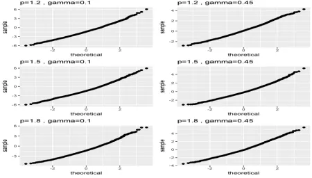
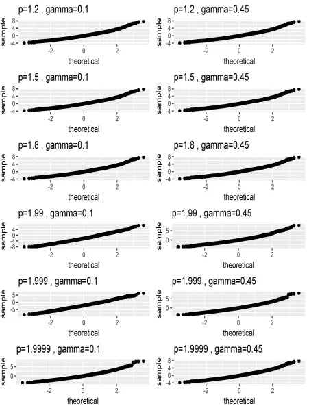
C

Additional simulations

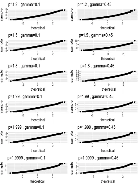
C.1 Extreme expectile estimation

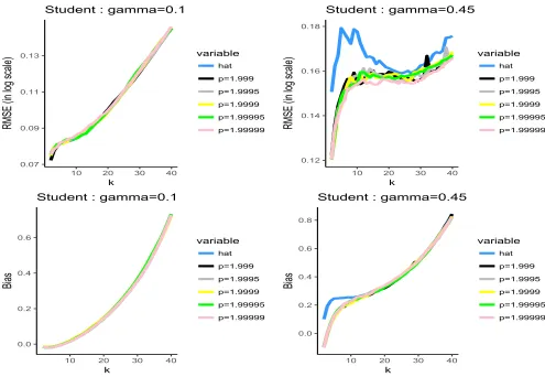
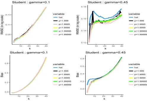
We concentrate here on extreme L2_{quantiles, or equivalently, expectiles. A comparison of the three estimators}

p

qW

αnp2qin (11), rq

W

αnp2q in (12) andqq

p

αnp2qin (13) (see the main paper) of the extreme expectile qαnp2qis shown in

Figures 1 and 2, where we present the evolution of their relative MSE (in log scale) in terms of the valuek. We used

the same considerations as in Section 6 for the choice ofpγn and the intermediate and extreme expectile levelsτnand

τ_n1 αn. The experiments employ the Fr´echet, Pareto and Student distributions with tail-indices γ P t0.1,0.45u

and various values ofpP p1,2qin the formulation (13) ofqqp αnp2q.

In the case of Fr´echet and Pareto distributions, we already know thatrq_αW_np2qbehaves better thanqpW_α_np2qin terms of relative MSE. In this case, it turns out that the accuracy of the estimatorqqpαnp2qis also superior toqp

W

αnp2qand