Consistent estimation in an implicit quadratic measurement error model

www.elsevier.com/locate/csda

Consistent estimation in an implicit quadratic

measurement error model

Alexander Kukush

_{, Ivan Markovsky}

_{, Sabine Van Hu-el}

Received 1 November 2002; received in revised form 30 October 2003; accepted 30 October 2003

Abstract

An adjusted least squares estimator is derived that yields a consistent estimate of the parameters of an implicit quadratic measurement error model. In addition, a consistent estimator for the measurement error noise variance is proposed. Important assumptions are: (1) all errors are uncorrelated identically distributed and (2) the error distribution is normal. The estimators for the quadratic measurement error model are used to estimate consistently conic sections and ellipsoids. Simulation examples, comparing the adjusted least squares estimator with the ordinary least squares method and the orthogonal regression method, are shown for the ellipsoid 7tting problem.

c

2003 Elsevier B.V. All rights reserved.

Keywords:Adjusted least squares; Conic 7tting; Consistent estimator; Ellipsoid 7tting; Quadratic measurement error model

1. Introduction

A parameter estimation problem occurs when the relation among some observed variables x1; : : : ; xn is described by a parameterized model. The parameters identify a unique model in a given model class, and the problem is to choose a model from the model class, given a set of observations{x(l)_}m

l=1, wherex(l) := [x1(l)· · ·x(l)n ] is thelth observed vector of variables. The model is selected according to certain performance criteria, speci7ed later.

∗_{Corresponding author. Tel.: +32-16-32-17-10; fax: +32-16-32-19-70.}

E-mail address:[email protected](I. Markovsky).

1_{On leave from National Taras Shevchenko University, Vladimirskaya st. 64, 01601, Kiev, Ukraine.} 0167-9473/$ - see front matter c2003 Elsevier B.V. All rights reserved.

We consider animplicit quadratic model,x_{Ax+bx+d=0,Asymmetric, relating} the variables x:= [x1· · ·xn]. It describes a second order surface

S(A; b; d) :={x∈Rn_{: xAx+bx+d= 0} (1)}

in Rn_{. The model is called implicit because there is no di-erence between dependent} and independent variables. The parameters are the symmetric matrix A, the vector b, and the scalar d and the model class is the set of all quadratic equations with an

n-dimensional variable.

IfA=0 andb= 0, then surface (1) is ahyperplane, and ifAis positive de7nite and 4d ¡ b_A−1_{b, then (1) is anelliptic surface. The set S(A; b; d) might be disconnected.}

Initially we will not make assumptions on the surface under estimation apart from the requirement of being a non-empty set. Later on we will specialize the results for the cases of conic section and ellipsoid estimation.

Without additional constraints imposed on the parameters, given a model in the model class, the model parameters are not unique: any multiple of a set of parameters

de7nes the same model. This makes the quadratic model, parameterized by A, b, and

d non-identi7able. To resolve the problem, we impose a normalizing condition, e.g.,

the parameters are assumed to satisfy the constraint

A2

F +b2+d2= 1: (2)

With this normalizing condition, the parameters are unique up to a sign.

The vector of variablesxis observed with additive error e=[e1· · ·en] and the error is described stochastically. The true value Hx= [ Hx1· · ·xHn] of the measured variables is assumed to satisfy the model for some unknown true values HA, Hb, and Hd of the parameters. This assumption de7nes a true modelin the model class. Models in which the variables are measured with additive noise x= Hx+eare calledmeasurement error models. Thus the model considered in the paper is an implicit quadratic measurement error model.

The quadratic model is linear in the parameters, so that the linear least squares technique can be applied. This corresponds to estimation criterion:

min A;b;d

m

l=1

(x(l)_Ax(l)_+bx(l)_+d)2_:

We will call the resulting estimator the ordinaryleast squares (OLS) estimator, in order to distinguish it from the adjusted least squares estimator, introduced later.

Due to the normalizing condition imposed on the parameters, the OLS problem is a quadratically constrained least squares problem and the necessary computation is to 7nd the smallest eigenvalue/eigenvector of a self-adjoint and positive de7nite linear operator. The presence of measurement errors in all the covariates, however, makes the OLS estimator biased, see, e.g., Carroll et al. (1995).

Another approach is the orthogonal regressionestimation. Let dist(x; S) be the

dis-tance from the point x to the set S. The orthogonal regression estimator is de7ned as

a global solution of the following optimization problem:

min A;b;d

m

l=1

The non-linearity of the model with respect to the measurements, implies the incon-sistency of this estimator as well, see the classical paper ofNeyman and Scott (1948)

and the discussion in (Fuller, 1987, p.250).

We assume that the measurement errorse(1)_{; : : : ; e}(m)_{are centered, uncorrelated among}

the measurement, and normally distributed, e(l) _{∼ N(0;H}2_{I) for all l, with noise}

variance H2_{. We consider both cases, when H}2 _{is given, and when H}2 _{is unknown.}

The stochastic description of the measurement errors can be viewed as a model

with parameter 2_{. Then the noise variance} 2 _{is a nuisance parameter of the}

model.

Using the noise model assumptions, we apply an adjustment procedure, see

Naidu (1990), that takes into account the quadratic structure of the model and

cor-rects the OLS estimate appropriately. The resulting estimator, called an adjusted least

squares (ALS) estimator, is consistent. Similar approach for consistent estimation is used in a bilinear model, see Kukush et al. (2003).

A nice feature of the ALS estimator is that its computation also requires the small-est eigenvector of a self-adjoint linear operator. This operator is obtained from the self-adjoint and positive de7nite operator used in the computation of the OLS estima-tor by applying the correction. If the measurement error variance H2 _{is a priori known,}

we give the correction operator in terms of H2_{. If however, H}2 _{is unknown, then it has}

to be estimated together with the model parameters. We propose a consistent procedure to estimate the unknown measurement error variance.

We use the ALS estimator, derived for the quadratic model, to solve theconic 5tting

and the ellipsoid 5tting problems. In the ellipsoid 7tting case, we obtain consistent

estimators for the parameters Ae and c of the ellipsoid described by the quadratic

model (x−c)_A

e(x−c) = 1, with Ae positive de7nite.

We point out several papers in which the ellipsoid 7tting problem is considered.

Gander et al. (1994) consider algebraic and geometric 7tting methods for circles and ellipses and note the inadequacy of the algebraic 7t on some speci7c examples. Later on, the given examples are used as benchmarks for the algebraic 7tting methods. Ellipsoid speci7c, as opposed to the more general conic 7tting method is 7rst

pro-posed in Fitzgibbon et al. (1999). The method incorporates the ellipticity constraint

into the normalizing condition and thus gives better results when an elliptic 7t is

de-sired. In Nievergelt (2001), a new algebraic 7tting method is proposed that does not

have as singularity the special case of a hyperplane 7tting; if the best 7tting manifold is aMne the method coincides with the total least squares method. Geometric meth-ods, minimizing the sum of absolute values of orthogonal deviations, are discussed in

Nyquist (1988).

A statistical point of view on the ellipsoid 7tting problem is taken in Kanatani

(1994),Cabrera and Meer (1996), and Zhang (1997). Kanatani proposed an unbiased estimation method, called a renormalization procedure. He uses an adjustment similar to the one in the present paper but his approach of estimating the unknown noise variance

is di-erent. Moreover, the noise variance estimate proposed inKanatani (1994) is still

Standard notation used in the paper is:Rfor the set of real numbers, Eefor the ex-pectation of the random variablee, Op(1) for a sequence of stochastically bounded ran-dom variables, N(0; V) for the zero mean normal distribution in Euclidean space with variance–covariance matrixV,min() (max()) for minimum (maximum) eigenvalue of the self-adjoint linear operator , AF for the Frobenius norm of the matrix A, and dist(x; y) is de7ned as x−y, where the norm is understood from the context. Throughout the paper S denotes the space of the n×n symmetric matrices. Speci7c notation is introduced in the text.

Section 2 de7nes the quadratic measurement error model. Sections 3 and 4 present, respectively, the OLS and the ALS estimators. In Section5, we state the consistency of

the ALS estimator with known noise variance, and in Section6, we consider the noise

variance estimation problem. The proofs of all results in Sections5 and6 are included

in the Appendix. Sections 7 and 8 consider two special cases of the quadratic model

estimation problem: conic section and ellipsoid 7tting. Section 9 shows simulation

examples for the ellipsoid 7tting problem. Conclusions are given in Section 10.

2. Quadratic measurement error model

Let HA∈S, Hb∈Rn_{, and Hd∈R be such that the set S( HA;b;HdH), de7ned in (1), is} non-empty and let the points Hx(1)_{; : : : ;xH}(m)_{, lie on the surface S( HA;b;H dH), i.e.,}

H

x(l)_AHxH(l)_{+ HbxH}(l)_{+ Hd= 0; for l= 1; : : : ; m: (3)}

The pointsx(1)_{; : : : ; x}(m)_{, aremeasurements of the points Hx}(1)_{; : : : ;xH}(m)_{, respectively, i.e.,}

x(l)_{= Hx}(l)_+e(l)_{; for l= 1; : : : ; m; (4)}

wheree(1)_{; : : : ; e}(m) _{are the corresponding measurement errors. We make the following} assumptions:

(1) the measurement errors e(1)_{; : : : ; e}(m) _{form a sequence of independent identically} distributed random vectors, and

(2) the distribution of e(l)_{, for all l= 1; : : : ; m, is normal N(0;H}2_In).

Here H2_{¿0 is the noise variance and I}

n is the n×n identity matrix.

The matrix HA∈S is the true value of the parameter A, while Hb∈Rn_{, and Hd∈R}1 are the true values of the parameters b and d, respectively. We assume that the true values of the parameters satisfy the normalizing condition (2).

3. Ordinary least squares estimator

The elementaryOLS cost function is

It measures the discrepancy of a single measurement pointxfrom the surfaceS(A; b; d). The OLS cost function/is the sum of the elementary cost function for all data points,

Qols(A; b; d) := m

l=1

qols(A; b; d; x(l)); for all A∈S; b∈Rn; d∈R: (5)

The OLS estimator Aˆols, ˆbols, ˆdols is de7ned as the global minimum point of (5),

subject to the normalizing constraint (2). We consider the parameter triple

:= (A; b; d)∈V

as a vector in the Hilbert space V:=S×Rn_{×R with inner product}

(A1; b1; d1);(A2; b2; d2):= trace(A

1A2) +b1b2+d1d2;

for all (A1; b1; d1)∈V; (A2; b2; d2)∈V:

With this notation, the optimization problem, we want to solve, is min

Qols() s:t: ; = 1: (6)

The cost function in (6) is a quadratic form of,

Qols() =ols; ;

whereols is a self-adjoint linear operator onV. Therefore the global minimum point

ˆ

ols:= ( ˆAols;bˆols;dˆols) = arg min

;=1Qols()

is a normalized eigenvector of ols, corresponding to the minimum eigenvalue

min(ols). In order to 7nd the operator ols : V → V, we calculate the derivative

Q

ols= dQols=d.

The derivative of qols(;x) with respect to is

q

ols(;x) = 2(xAx+bx+d)(xx; x;1)

= 2(xx_{; x;1); (xx; x;1):}

It de7nes a self-adjoint and positive semide7nite linear operator ols(x) on V, ols(x):=(xx_{; x;1); (xx; x;1) for all ∈V:}

Thus

ols=

m

l=1

ols(x(l)): (7)

vector of the elements in the upper triangular part ofAtaken column-wise. There exists a matrix M∈R(nA+n+1)×(nA+n+1) associated with the operator Qols, such that

Qols() =    

vecs(A)

b d

   

M

   

vecs(A)

b d

  

 for all A∈S; b∈Rn; d∈R: (8)

Using the matrix representation (8), the whole derivation of the OLS estimator, and subsequently the one of the ALS estimator, can be carried out in linear algebra

notation. We use the matrix representation approach inMarkovsky et al. (2002), where

the computation of the estimators is treated. In this paper, we use the abstract operator notion.

4. ALS estimator withknown noise variance

The OLS estimator is readily computable but it is inconsistent. We propose an adjustment procedure, that de7nes a consistent estimator. The proposed approach is

due toKukush and Zwanzig (2002), and it is related to the method of corrected score

functions, (see Carroll et al., 1995, Section 6.5). The model (3) is quadratic and similar

adjustment for a bilinear model, arising in motion analysis, is proposed in Kukush

et al. (2002)

We de7ne the elementaryALS cost function qals(;x) by

Eqals(; Hx+e) =qols(; Hx) for all ∈V and Hx∈Rn; (9)

whereeis N(0;H2_{In) distributed. The ALS cost functionis the sum of the elementary} ALS cost functions for all data points

Qals() := m

l=1

qals(;x(l)) for all ∈V:

The ALS estimator ˆals is de7ned as the global minimum point of the following optimization problem:

min

Qals() s:t: ; = 1: (10)

The solution of (10) is described in the following theorem.

Theorem 2. The ALS estimator ˆals is the normalized eigenvector of

als:= m

l=1

als(x(l)_);

corresponding to min(als), where

als(x)= (g1(x)[A] +g2(x)[b] +g3(x)[d];

the functions gs, s= 1; : : : ;6 are de5ned by

[g1(x)[A]]_pq= n

i;j=1

aijfijpq(x) for all A∈S; (12)

[g2(x)[b]]pq= n

i=1

bifipq(x) for all b∈Rn; (13)

g3(x)[d] = (xx−H2In)d for all d∈R; (14)

[g4(x)[A]]p= n

i;j=1

aijfijp(x) for all A∈S; (15)

g5(x)[b] = (xx_−H2_{In)b for all b∈R}n_{; (16)}

g6(x)[A] =xAx−H2 trace(A) for all A∈S; (17)

the functions fijpq in (12)are de5ned by

• if alli, j,p,q are di7erent,then fijpq(x) =xixjxpxq;

• if i=j=p, q=i (with permutations), then fiiiq(x) =xqt3(xi);

• if i=j=p=q, then fiiii(x) =t4(xi);

• if i=j,p=q, i=p,then fiipp(x) =t2(xi)t2(xp);

• if i=j and i,p, q are di7erent, then fiipq(x) =xpxqt2(xi);

the functions fijp in(13) and (15) are de5ned by

• if i=p=q,then fiii(x) =t3(xi);

• if i=p,p=q (with permutations), then fiiq(x) =t2(xi)xq;

• if i; p; q are di7erent, then fipq(x) =xixpxq,

and the functionstk,k= 1; : : : ;4 are de5ned by t1(') ='; t2(') ='2−H2; t3(') ='3−3'H2;

and t4(') ='4−6'2H2+ 3 H4: (18)

Proof. Consider Eq. (9), which implicitly de7nesqals. It is the followingdeconvolution

problem:

1 2(H2

n=2 ∞

−∞ · · ·

_∞

−∞ qals(; Hx+e)

n

i=1

exp

− e2i

2 H2 de1· · ·den= qols(; Hx):

(19) Since qols(; Hx) is quadratic in , Eq. (19) holds for all inV, and the integral does

not depend on ,qals must be quadratic in for all x. Thus

where als(x) is a self-adjoint linear operator on V, such that

E als( Hx+e) = ols( Hx) for all Hx∈Rn_{: (20)}

Then Qals is also quadratic in ,

Qals() =als; for all ∈V;

whereals:=m_l=1 als(x(l)), and theALS estimatorˆalsis the normalized eigenvector of als, corresponding to min(als).

Now, we describethe operator als(x) that solves (20). Solving a general deconvolu-tion problem is not possible analytically. In our case, however, the normality assumpdeconvolu-tion for the noise makes the problem tractable. Looking at the right-hand-side of (20),

ols(x)= (x_{Ax+xb+d)(xx; x;1) where = (A; b; d);}

we see that the problem splits into six independent problems

E als( Hx+e) =hs(x)[] for all Hx∈Rn and for s= 1; : : : ;6; (21)

wherehi(x)[] are the summands in the expansion of ols(x):

h1(x)[A] :=xx_{(xAx); h2(x)[b] :=xx(xb); h3(x)[d] :=xxd;}

h4(x)[A] :=x(x_{Ax); h5(x)[b] :=xxb; h6(x)[A] :=xAx:} Let

g1:S→S; g2:Rn×1→S; g3:R→S;

g4:S→Rn×1; g5:Rn×1→Rn×1; g6:S→R;

be the solutions of (21), then the solution of (20) is given by (11).

Some of the functions gs can be found by inspection. For example, the solution of

the deconvolution equation for h3 is (14). Similarly, the solution of the deconvolution equation for h6 is (17). Due to the symmetry, g2= (g4)∗ _{and g3= (g6)}∗_{, where g}∗

denotes the conjugate operator of g.

Next, we describe the other functions gs. LetA= [aij]. Then

[h1(x)[A]]_pq= n

i;j=1

aijxixjxpxq for all A∈S:

Therefore the solution of the corresponding deconvolution problem is (12), wherefijpq is a polynomial of the fourth order with the property

Efijpq( Hx+e) = HxixHjxHpxHq: (22)

The polynomials tk:R→R, k= 1; : : : ;4, de7ned in (18), have the property

Etk( H'+ ˜') = H'k_{; for k= 1; : : : ;4; and for all H'∈R; and ˜'∼N(0;H}2_):

Then the functions fijpq de7ned in the theorem have the desired property (22).

Similarly for

[h2(x)[b]]_pq= n

i=1

the solution of the deconvolution problem (21) is (13), where fipq are de7ned in the theorem. Finally,

[h4(x)[A]]_p= n

i;j=1

aijxixjxp;

and the solution of the deconvolution problem (21) is (13). Thus the adjusted operator

als(x) in V is described thoroughly.

Remark 3. If the given data is noise free, i.e., H= 0, then x(l)_{= Hx}(l) _{for all l, and}

the solution of the deconvolution equation (19) isqols. In this case, the ALS estimator

coincides with the OLS estimator.

5. Consistency of the ALS estimator

Let n:= dimV=n(n+ 1)=2 +n+ 1 = (n+ 1)(n+ 2)=2, and let

1( Hols=m)¿2( Hols=m)¿· · ·¿n( Hols=m) = 0

be the eigenvalues of Hols=m, where Hols is given in (7) with Hx(l). We need the

following assumptions:

(iii) There existsm0¿1 and *0¿0, such that

n−1( Hols=m)¿*0 for allm¿m0:

(iv) There exists a constant *1¿0 and a number +∈[0;1), such that 1

m

m

l=1

xH(l)6_6*

1m+ for all m¿1:

Assumption (iii) is a contrast condition, see the discussion in Kukush and Zwanzig (2002). Similar condition is used in Kukush et al. (2003). Assumption (vi) is a re-striction from above. If HA is positive de7nite and 4d ¡ b_A−1_{b, then S( HA;b;}H _dH_{) is an}

elliptic surface, which is bounded, and (iv) holds with += 0.

Let

dist(1; 2) :=1−2V

and

dist(1;{±2}) := min{dist(1; 2);dist(1;−2)}:

Theorem 4(Strong consistency). Assume that conditions(i)–(iv)hold.Then the ALS estimator alsˆ and the true value H := ( HA;b;H dH) satisfythe following convergence property:

Corollary 5. Under the conditions (i)–(iv),

dist( ˆals;{±H}) =_m(1−+)=21 Op(1); (23)

and for each , ¿0,

dist( ˆals;{±H})m(1−+)=2−,→0 as m→ ∞; a:s: (24)

Corollary 5 shows that for unbounded sequence {xH(l)_{; l¿1}, there may be a loss}

of order in the rate of convergence of the estimator. But if += 0, then the estimator is

√

m-consistent, i.e.,

dist( ˆals;{±}H ) = Op(1)=√m: (25)

The statement of Theorem 4 is one of the main contributions of the paper. Adjust-ment procedures, similar to the one described in Section 4, already appeared in the

literature; 7rst proposed in Kanatani (1994) and later developed in Cabrera and Meer

(1996)andZhang (1997). In these papers, however, consistency of the ALS estimator is not proven. Instead the notion of unbiasedness is used, i.e.,Eˆals= H. In the present

context, however, bias is not well de7ned for the reason that the expectation of the ALS estimator does not exist.

Suppose we draw N realizations of the measurement errors and compute the ALS

estimates, for the corresponding data sets. Let ˆals;k be the estimate for the kth data set. Then

1

N

N

k=1

ˆals;k → ∞ as N→ ∞:

In the context of a linear measurement error model, the fact thatEˆals does not exist

is stated in (Fuller, 1987, Exercise 13, p. 28). It is proven for a multivariate linear

measurement error model in the unpublished manuscript Cheng and Kukush (2001).

6. Consistent estimator in the case of unknown noise variance

Suppose we misspeci7ed the noise variance. The true value is H2 _{and we construct}

the operator2 :=als, regarding 2 to be the true value of that parameter. We study

the di-erence

E_H2 2( Hx+e)−E2 2( Hx+e);

where EH2 and E2 denote the expectation with e ∼ N(0;H2I_n) and e ∼ N(0; 2I_n),

respectively.

Consider the polynomials tk('), k= 2;3;4, given in (18). Assuming 2 to be the true value of the noise variance, we have

t2(') ='2₋2_;

which can be written as

so that for '= H'+ ˜', with ˜'∼N(0;H2₎

EH2t2( H'+ ˜') =E_H2(( H'+ ˜')2−H2+ ( H2−2)) = H'2_{+ ( H}2₋2_{) for all '∈R:} Next, for the polynomial t3, we have

t3(') ='3_−3'2

='3_−3'H2_{+ 3'( H}2₋2_); so that

EH2t3( H'+ ˜') =E_H2(( H'+ ˜')3−3( H'+ ˜') H2+ 3( H'+ ˜')( H2−2)) = H'3_{+ 3 H'( H}2₋2_):

Finally for the polynomial t4, we have

t4(') ='4_−6'22_{+ 3}4

='4_−6'2_H2_{+ 3 H}4_{+ 6'}2_{( H}2₋2_{)−3( H}4₋4_); so that

EH2t4( H'+ ˜') = H'4+ 6( H2−2)E_H2('+ ˜')2−3( H4−4) = H'4_{+ 6( H}2₋2_{)( H'}2_{+ H}2_{)−3( H}4₋4_): Thus

EH2t_k( H'+ ˜') = Hxk_i + ( H2−2)z_k( H'; H2−2); for k= 2;3;4; with

z2(x; H2−2) := 1; z3(x; H2−2) := 3x; and

z4(x; H2−2) := 6(x2+ H2)−3( H2+2) = 6x2_{+ 3( H}2₋2_):

For the polynomials fijp, de7ned in Section 4, we have

EH2fijp( Hx+e) = Hx_ixH_jxH_p+ ( H2−2)zijp( Hx; H2−2);

wherezijp does not depend on H2−2 or the dependence is linear, e.g., for i=j=p, we have

EH2fiip( Hx+e) = (E_H2t2( Hx_i+ei)) Hx_p

= ( Hxi)2_xH

p+ ( H2−2) Hxp;

then ziip= Hxp. Similarly, the polynomials zijpq( Hx; H2−2) are de7ned by

For the operator 2(x), which is constructed starting from the value2, we have

EH2 2( Hx+e) = ols( Hx) + ( H2−2)z( Hx; H2−2);

where z= : (zA; zb; zd) is a certain self-adjoint operator on V, which either depends linearly on H2₋2 _{or does not depend on H}2₋2_{. For example z}

d does not depend on H2₋2_{. Indeed}

zd= trace(A); because for x= Hx+e,

EH2(g5(x; A) +xb+d) = ( HxAxH+xb+d) + ( H2−2) trace(A): Now, for the sum over mobservations, the operator Z( H2₋2_{) is de7ned by}

Z( H2₋2_{) :=}m l=1

z( Hx(l)_{; H}2₋2_);

and then

E_H22= H_ols+ ( H2−2)Z( H2−2):

We need the following assumptions in order to estimate H2_:

(v) There exists a number 00∈[1; n] and*2¿0, such that 1

m

m

l=1 ( Hx(l)

00)26*2 for all m¿1:

We de7ne

Fm(1) := ( Hols+_m1Z(1)) for 1∈R:

(vi) For each v ¿0 and *∈(0; v), lim inf

m→∞ |1|∈[*min2_;v2_]|min(Fm(1))|¿0:

We introduce the score function

Um(2_{) :=} min

2

m for 062¡∞: (26)

Lemma 6. Assume that conditions (i)–(iii) and (vi) hold.Then with probabilityone Um(0)¿0 and lim

2_→∞Um(

2_{) =−∞:}

We de7ne an estimator ˆ2_{, as a random variable, such that}

Um( ˆ2) = 0; a:s: (27)

The functionUm is continuous in 2∈[0;∞), and by Lemma6 there exists a solution

The reason in de7nitions (26) and (27) is as follows. For large m,

Um( H2)≈min _H

ols m = 0:

On the other hand, for large m and misspeci7ed noise variance 2_{= H}2_, Um(2_)≈minolsH + ( H2−2)Z( H2−2)

m :

By condition (vi),Um(2) is asymptotically separated from 0. Thus we expect that the solution of (27) is close to H2_.

Now, we prove that the estimator 2 _{is bounded in m, a.s.}

Lemma 7. Assume that conditions (i)–(v) hold. Then

sup m¿1ˆ

2

m¡∞; a:s:

Lemma 8. Assume that conditions (i)–(vi) hold. Then

ˆ

2_→H2_{; as m→ ∞; a:s:;}

where H2 _{is the true value of the parameter} 2_.

(vii) There exists an*3, such that 1=mm_l=1 xH(l)2_{6*3, for all m¿1.}

With unknown H2_{, the ALS estimator ˆ is de7ned as a normalized vector satisfying} ˆ

2ˆ= 0.

Theorem 9. Let H2 _{be unknown. Assume(i)–(iv), (vi), and (vii). Then} dist( ˆ;{±H})→0 as m→ ∞; a:s:

7. Fitting conic sections

Now, we suppose that the true surface belongs to the class of surfaces

C(Ac; c) ={x∈Rn: (x−c)Ac(x−c) = 1} (28)

for some true values HAc and Hc of the parameters Ac and c. Here Ac (“c” stands for conic) is a non-singular symmetricn×n matrix, andc∈Rn _{is the center of the surface.} The equation de7ningC(Ac; c) can be written as

x_A

cx−2(Acc)x+cAcc−1 = 0

or, with 5:= (Ac2F +2Acc2+ (cAcc−1)2)1=2,

x_(A

c=5)x−2(Acc=5)x+ (cAcc−1)=5= 0: De7ne the new parameters

A:=Ac

5 ; b:=−2 Acc

5 and d:=

c_A cc−1

5 :

We can renew the original parameters Ac and c from A, b, and d, that satisfy (2)

by

c=−1₂A−1_{b; and Ac=} 1

c_Ac−d A: (29)

Note that 5=c_{Ac−d is non-zero.}

Now suppose that we observe the points x1_{; : : : ; x}m_{, given in (4). The true values}

H

x1_{; : : : ;xH}m_{, satisfy}

( Hx(l)_{−cH)AcH ( Hx}(l)_{−cH) = 1 for l= 1; : : : ; m: (30)}

We rewrite (30) in the form H

x(l)_AHxH(l)_{+ 2 HbxH}(l)_{+ Hd= 0 for l= 1; : : : ; m;}

where

H

A=AH₅c; bH=−2AH₅cH; dH=cHAH₅cH−1;

and

5=||Ac||H 2

F +||2 HAcc||H 2+ ( HcAcH cH−1)2:

Let the noise variance H2 _{be unknown. Assume (i)–(vi). Then}

dist( ˆ;{±}H )→0 asm→ ∞; a:s:; (31)

where ˆ:= ( ˆA;b;ˆdˆ) is the ALS estimator of the parameters HA, Hb, and Hd. The estimator of the parameters HAc and Hc is

ˆ

c=−1₂Aˆ−1_{bˆ and Aˆ}

c= 1

ˆ

c_Aˆ_cˆ−dˆ A:ˆ (32)

Under (i)–(vi), the estimators are well de7ned for m¿m0(!), a.s., and

Aˆc−AHc2F+cˆ−cH2→0 as m→ ∞; a:s: Indeed from (31), we have, see the formulae in (29), that

ˆ

c=−1₂Aˆ−1_{bˆ→ −}1

2AH−1bH= Hc as m→ ∞; a:s: And

ˆ

Ac= 1

ˆ

c_Aˆ_cˆ−dˆAˆ→

1 H

c_AH_cH−dHAH= HAc:

It is important here that HAc is non-singular. If ˆAis singular, then the estimators ˆAcand ˆ

c are not de7ned, and if ˆA is non-singular but ˆb_{( ˆA)}−1_bˆ_{= ˆd, then ˆAc is not de7ned.}

8. Estimation of ellipsoid

We specialize the case described in Section 7 for elliptical surface. Let in (28)

Ac=Ae, where Ae (“e” stands for elliptic) is a positive de7nite matrix. Then C(Ac; c) is an elliptical surface. The true value HAe of the parameter Ae is positive de7nite.

We can improve estimator (32) in this case. The problem is thatAccan be inde7nite. We do the following additional step. Let

ˆ

Ac=

n

i=1

ˆ

ivˆivˆi

be the EVD of ˆAc, given in (32). Then we set ˆ

Ae:=

i: ˆi¿0

ˆ

ivˆivˆi :

The estimator ˆAe is positive semide7nite. Moreover as HAe is positive de7nite now, we have

Aeˆ −AeH F6Acˆ −AeH F;

and the estimator ˆAe is a strongly consistent estimator of HAe, i.e., ˆAe→AHe, asm→ ∞,

a.s.

9. Simulation examples

In this section, we show simulation examples for the ellipsoid 7tting problem. The aim is to illustrate the consistency results of the paper and to compare the ALS es-timator with the OLS and the orthogonal regression eses-timators. All experiments are carried out in the environment of MATLAB.

De7ne the (truncated) average relative errors of estimation by

H

eA :=_N1 N

k=1

min

Aˆe;k−AHeF

AeH F ;1

; eHc:= _N1 N

k=1

min

cˆk−cH

cH ;1 ; and

H

e:= _N1 N

k=1

min

|ˆk−|H H

;1 ;

where ˆAe;k, ˆck, and ˆk are the estimates obtained on thekth repetition of the estimation experiment. In each repetition, di-erent noise realization is used. The reason for using the truncated average of the relative errors of estimation is that the expectation of the

relative errors does not exist, see the discussion in Section 5. We have selected the

truncation level to 100%.

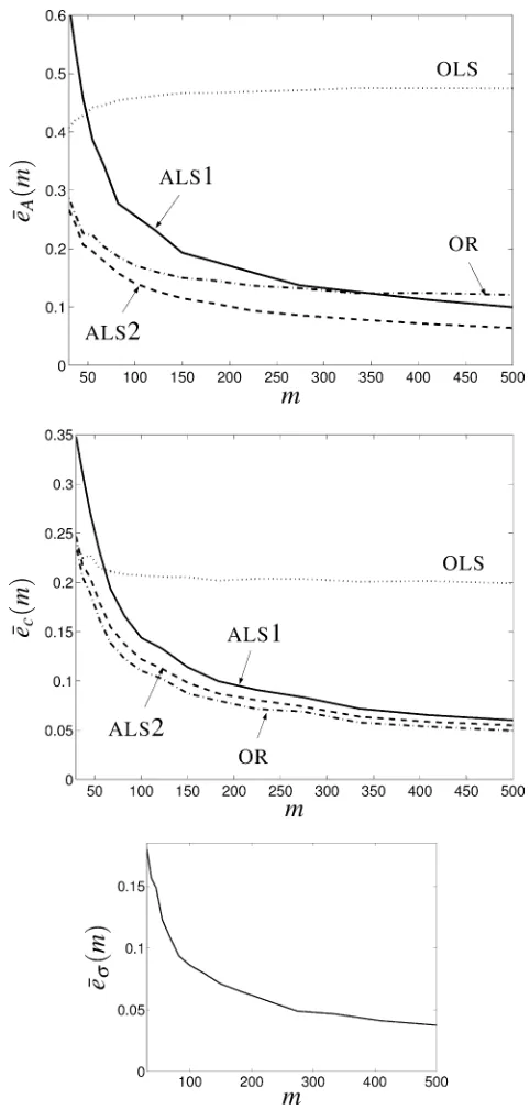
In Fig.1, we showasymptotic plotsof HeA, Hec, and Heas a function of the sample size

m. The true data points Hx(l) _{are equidistantly spaced on the boundary of the ellipsoid}

Fig. 2. Average relative error of estimation as a function of the noise standard deviation H. OLS—ordinary least squares, OR—orthogonal regression, ALS1—ALS estimator with known H2_{, and “ALS2”—ALS} esti-mator with estimated noise variance.

for each value of m. The initial approximation for the computation of the orthogonal regression estimator is the OLS estimate.

The OLS estimator is clearly biased and the error of the ALS estimator is

√

m-consistent. Note that the ALS estimator with unknown true noise variance (ALS2) performs consistently better than the ALS estimator with known true noise variance (ALS1).

Fig. 2 shows the relative errors of estimation as a function of the noise standard

deviation. The setting of the experiment is as before. The noise standard deviation is increased from 0.1 to 0.6 and the sample size is 7xed tom=100 data points. The initial approximation for the computation of the orthogonal regression estimator is again the OLS estimate.

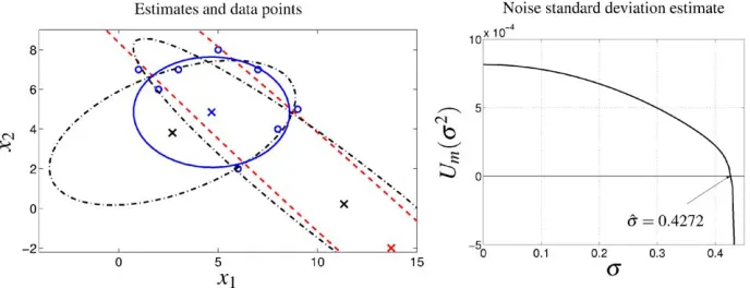
The last experiment shows the performance of the estimators on a test example from

Gander et al. (1994). The example is used in Gander et al. (1994) to illustrate the inadequacy of the algebraic 7tting method and to show the advantage of the orthogonal regression method.

Given are data points only; even if they are generated with a true model, we do

not know it. For this reason the comparison is visual. Fig. 3, left, shows the data

points with the estimated ellipses superimposed on them. The dashed line represents the OLS estimate, the dashed–dotted lines, the orthogonal regression estimates (when initial approximation is the OLS estimate and the ALS estimate), and the solid line,

the ALS estimate. The data points are marked with circles (◦) and the centers of the

estimated ellipses are marked with crosses (×).

The orthogonal regression estimator is inUuenced by the initial approximation.

Us-ing the OLS estimate as initial approximation, the optimization algorithm (MATLAB’s

Fig. 3. Test example fromGander et al. (1994). Dashed line—OLS estimate, dashed–dotted lines—orthogonal regression estimates (with initial approximation, the OLS estimate and the ALS estimate), solid line—ALS estimate,◦—data points,×—centers of the estimated ellipses.

m= 8 data points, the ALS estimator gives good estimate and is comparable with the orthogonal regression estimate, corresponding to the global minimum point.

Fig. 3, right, shows the functions Um used for the estimation of the noise

vari-ances. From the given data, we compute an upper bound of the true noise standard deviation

v:=

1

n

1

m

m

l=1 x(l)

c 2−₁₆min_l6mx(cl)2

1=2

where x(l)

c :=x(l)−_m1 m

k=1 x(k)_;

and use a bisection method, seeGill et al. (1999), to 7nd a zero of Um in the interval

∈[0; v]. For the example there is a unique zero in the interval [0; v], which corresponds to the noise standard deviation estimate.

10. Conclusions

We have presented a consistent estimator for the parameters of an implicit quadratic measurement error model. The method used is the adjustment procedure is due to

Kukush and Zwanzig (2002). We give conditions, under which the estimator is strongly consistent. The adjustment needs the true noise variance. We show, however, a pro-cedure to estimate the noise variance. This propro-cedure de7nes a consistent estimator of the model parameters with unknown noise variance. The quadratic model is used for the conic section and ellipsoid 7tting problems. We give simulation results for the ellipsoid estimation that illustrate the consistency of the ALS estimator.

the normalizing conditions for the parameters a-ects the eMciency of the estimator. In particular, what is the optimal normalizing condition in terms of eMciency.

Acknowledgements

A. Kukush is supported by a postdoctoral research fellowship of the Belgian of-7ce for Scienti7c, Technical and Cultural A-airs, promoting Scienti7c and Techni-cal Collaboration with Central and Eastern Europe. S. Van Hu-el is a full professor and I. Markovsky is a research assistant with the Katholieke Universiteit Leuven. I. Markovsky is supported by a K.U. Leuven doctoral scholarship.

This paper presents research results of the Belgian Programme on Interuniversity Poles of Attraction (IUAP Phase V-22), initiated by the Belgian State, Prime Minister’s OMce—Federal OMce for Scienti7c, Technical and Cultural A-airs, of the Concerted Research Action (GOA) projects of the Flemish Government MEFISTO-666 (Mathe-matical Engineering for Information and Communication Systems Technology), of the IDO/99/03 and IDO/02/009 projects (K.U. Leuven) “Predictive computer models for medical classi7cation problems using patient data and expert knowledge”, of the FWO projects G.0078.01 and G.0270.02.

Appendix.

Proofs of the statements

Proof of Theorem 4. Under assumption (iv), 1

m

m

l=1

fijpq( Hx(l)+e(l))−_m1 m

l=1

Efijpq( Hx(l)+e(l))→0 asm→ ∞; a:s:

To show this, we will restrict our attention to the most unfavorable casei=j=p=q. Then fiiii(x) =x4i −6x2iH2+ 3 H4 and we have to show that

1

m

m

l=1

((x(l)_i )4_−6(x(l)

i )2H2+ 3 H4)− _m1 m

l=1

( Hx(l)_i )4_{→0 as m→ ∞; a:s: (33)}

Now, x_i(l)= Hx(l)_i +e(l)_i . Then (x(l)_i )4_−6(x(l)

i )2H2+ 3 H4−( Hx(l)i )4

= 4( Hx(l)_i )3_e(l)

i + 6( Hx(l)i )2((e(l)i )2−H2)

+ 4 Hx(l)_i (e(l)_i )3_{−12 Hx}(l)

i e(l)i + ((e(l)i )4−6ei(l)H2+ 3 H4): (34) Here the most unfavorable summand is 4( Hx(l)_i )3_e(l)

i . We consider

7m=_m1 m

l=1

By the Rosenthal inequality, see Rosenthal (1970), we have that

E|7m|2+8= _m2+1₈E

m l=1

( Hx(_il))3_e(l)

i

2+8

6_m2+1_{8 m}

l=1

( Hx(_il))6 _(2+8)=2

C(8;H);

for arbitrary 8 ¿0, where the constant C(8;H) depends only on 8 and H. Next, by

(iv) we have

E|7m|2+8= const_m1+1₈₌₂

1 m m l=1 xH(l)6

1+8=2

6const 1

m(1+8=2)(1−+):

We choose and 7x8large enough in order to have the inequality (1+8=2)(1−+)¿1.

Then ∞_m=1E|7m|2+8¡∞, therefore by the Chebyshev inequality and the Borel–

Cantelli lemma, see Papoulis (1991), 7m → 0, as m → ∞, a.s. In a similar way

the other summands of (34) being averaged for l= 1; : : : ; m, tend to zero as m→ ∞, a.s., e.g., for

9m:= _m1 m

l=1

( Hx(_il))2_((e(l)

i )2−H2)

we have

E|9m|2+86const_m1+1₈₌₂

1 m m l=1 xH(l)4

1+8=2

6const_m1+1₈₌₂

1 m m l=1 xH(l)6

4=6(1+8=2)

6const 1

m(1+8=2)(1−2+=3) for 8 ¿0;

and the inequality (1 +8=2)(1−2+=3)¿1, which holds for large 8, implies 9m→0, as m→ ∞, a.s. Thus (33) holds.

ButEfijpq( Hx(l)_+e(l)_{) = Hx}(l)

i xH(jl)xHp(l)xH(ql), therefore

1

m

m

l=1

fijpq( Hx(l)+e(l))−_m1 m

l=1

H

x(_il)xH(_jl)xH(l)

Similar convergence holds for fijp( Hx(l)). This implies that for H

ols:= m

l=1 ols( Hx);

we have

_m1 als−_m1Hols→0; as m→ ∞; a:s: (36) Let

1(als=m)¿2(als=m)¿· · ·¿n(als=m)

be the eigenvalues of als=m. Suppose that als=m−Hols=m6*, and * ¡ *0, where

*0 comes from assumption (iii). Then _n

(als=m)−n( Hols=m)6

_m1 als−_m1 Hols6*;

therefore|n(als=m)|6*. By making use of the perturbation theorems of eigenvectors,

as given inWedin (1972) andDavis and Kahan (1970), we have for the corresponding normalized eigenvectors ˆals and H that

dist( ˆals;{±}H )6 *

n−1( Hols=m)−n( Hals=m)

6_* *

0−*= :L(*); (37)

and lim*→0L(*) = 0. This relation and convergence (36) prove the statement.

Proof of Corollary5. The convergence of (35) was studied in the proof of Theorem 4. Consider for the most unfavorable summands

7m:= _m1 m

l=1

( Hx(_il))3_e(l)

i :

It was shown that for each 8 ¿0, there is a constant *8, that depends only on 8, for

which

E|7m|2+86 _m(2+8*₎₍₁8₋₊₎₌₂: (38)

Therefore

|7m|2+8m(2+8)(1−+)=2= Op(1); and

7m=_m(1−+)=21 Op(1):

The other summands in (35), which have expectation zero, also satisfy this relation. Then

and from (37), we have

dist( ˆals;{±}H ) =_m1 als−_m1 olsH Op(1)

=_m(11₋₊₎₌₂Op(1):

Now, we show (24). From (38), we have

E(m*_|7

m|2+8)6 _m(2+8)(1*+_−+)=2−*; for * ¿0:

For large enough8, we have

(2 +8)(1−+)=2−* ¿1;

and then by the Chebyshev inequality and the Borel–Cantelli lemma, see Papoulis

(1991),

m*_|7

m|2+8→0 as m→ ∞; a:s:; and

|7m|m*=(2+8)→0 as m→ ∞; a:s:;

when * ¡(2 +8)(1−+)=2−1. Fix 0¡ , ¡(1−+)=2. Then

*=(2 +8) = (1−+)=2−2=(2 +8);

and

2=(2 +8) =, for 8= 2=,−2:

Then

|7m|m(1−+)=2−,→0 as m→ ∞; a:s:; and

_m1 als−_m1 olsH m(1−+)=2−, _{→0 as m→ ∞; a:s:} Then (37) implies statement (24).

Proof of Lemma6. We have

2=ols for 2= 0;

therefore

Um(0) =min

ols m ¿0:

(In practice, for noisy observations and for m ¿ n, ols is strictly positive de7nite

Now introduce the unit vector h∈V,

h:= (0; e1;0);

wheree1∈Rn×1 is e1:= [1 0· · ·0]. We have for the scalar product in V,

1

m2h; h

=

1

mH2h; h

+ H2₋2_;

and

1

m2h; h

→ −∞ as 2 _{→ ∞; a:s:}

But

min ₁

m2 6

₁

m2h; h

;

and this implies the second statement in Lemma 6.

Proof of Lemma7. Let 00 be the constant from condition (v) and let h0∈V be the unit vector

h0= (0; e00;0);

where e00∈Rn is e00 := [0· · ·0 1 0· · ·0], with 1 on the 00th position. From the

de7nition of ˆ2_{, we have}

06

1

mˆ2h0; h0

=

1

mH2h0; h0

+ H2_−ˆ2_;

and, see (36),

ˆ

2_6H2₊1

molsH h0; h0

+ o(1) as m→ ∞; a:s:

Then by condition (v),

ˆ

2_6H2₊ 1 m

m

l=1

( Hx(l)

00)2+ o(1)

6H2_+*

2+ o(1):

Proof of Lemma8. It can be shown that for each v ¿0,

Em(v; !) := sup

062_6v2

_m1 2(!)−F_m( H2−2)→0 as m→ ∞; a:s: (39) We 7x !∈<, for which ˆ2

m(!) is bounded in m, and for which the convergence (39)

holds for every v∈N. The sequence {ˆ2

m(!); m¿1} belongs to the interval [0; v2]. Here v=v(!)∈N, and we assume that v ¿H. We have from (27) and (39) that

Consider any convergent subsequence {ˆ2

m(k)(!); k¿1}, say ˆm(k)2 (!)→2∞, ask→

∞. Suppose that 2

∞= H2. Then for certain m1=m1(!) and ,=,(!)¿0, we have for all m(k)¿m1, that

|min(Fm(k)( H2−ˆ2))|¿ min

,2_6|1|6v2|min(Fm(k)(1))|: (41) But from (40) and (41), we have for m(k)¿m1, that

min

,2_6|1|6v2|min(Fm(k)(1))|6Em(k)(v; !)→0 as k→ ∞:

This contradicts assumption (vi). Therefore2

∞= H2. Thus each convergent subsequence

of {ˆ2

m(!); m¿1} converges to H2, therefore ˆ2m(!)→H2, as m→ ∞. We 7xed ! from the set <0 of probability one, therefore ˆ2m→H2, a.s.

Proof of Theorem9. The proof is similar to the proof of Theorem2 of Kukush et al. (2003). Due to the quadratic structure of2 with respect to 2 and due to (vii), we

have for each v ¿0,

sup

m¿1 062 sup 16v2; 06226v2

|2 1−22|6,

_m1 2

1−

1

m22

→0 as ,→ ∞; a:s:

This means that the functions {2=m; 2∈[0; v2]; m¿1} are equicontinuous, a.s.

Therefore, see Lemma 8, for v2_{(!) := sup}

m¿1ˆ2m(!) we have

_m1 ˆ2− 1

mHols

6_m1 ˆ2− 1

mH2

+_m1 H2− 1

mHols

6sup

m¿1 06sup2_6v2_(!) |2_−H2_|6|ˆ2

m−H2|

_m1 2− 1

mH2

+_m1 H2− 1

mHols

→0 as m→ ∞; a:s:

Then like in the proof of Theorem 4, we obtain that dist( ˆ;{±}H )→0, as m→ ∞,

a.s.

References

Cabrera, J., Meer, P., 1996. Unbiased estimation of ellipses by bootstrapping. IEEE Trans. Pattern Anal. Mach. Intell. 18 (7), 752–756.

Carroll, R.J., Ruppert, D., Stefanski, L.A., 1995. Measurement error in nonlinear models. no. 63. Monographs on Statistics and Applied Probability. Chapman & Hall/CRC, London/Boca Raton.

Cheng, C., Kukush, A., 2001. Nonexistence of the 7rst moment of the adjusted least squares estimator in multivariate errors-in-variables model, unpublished manuscript.

Davis, C., Kahan, W.M., 1970. The rotation of eigenvectors by a perturbation III. SIAM J. Numer. Anal. 7, 1–46.

Fuller, W.A., 1987. Measurement Error Models. Wiley, New York.

Gander, W., Golub, G.H., Strebel, R., 1994. Fitting of circles and ellipses: Least-squares 7tting of circles and ellipses. BIT 34 (4), 558–578.

Gill, P.E., Murray, M., Wright, M.H., 1999. Practical Optimization. Academic Press, NY, USA.

Kanatani, K., 1994. Statistical bias of conic 7tting and renormalization. IEEE Trans. Pattern Anal. Mach. Intell. 16 (3), 320–326.

Kukush, A., Zwanzig, S., 2002. On consistent estimators in nonlinear functional EIV models. In: Van Hu-el, S., Lemmerling, P. (Eds.), Total Least Squares and Errors-in-Variables Modeling: Analysis, Algorithms and Applications. Kluwer, USA, pp. 145–155.

Kukush, A., Markovsky, I., Van Hu-el, S., 2002. Consistent fundamental matrix estimation in a quadratic measurement error model arising in motion analysis. Comput. Statist. Data Anal. 41 (1), 3–18. Kukush, A., Markovsky, I., Van Hu-el, S., 2003. Consistent fundamental matrix estimation in a quadratic

measurement error model arising in motion analysis. Metrika 57 (3), 253–285.

Markovsky, I., Kukush, A., Van Hu-el, S., 2002. Consistent least squares 7tting of ellipsoids. Technical Report 02–116, Department of EE, K.U. Leuven, (Numer. Math. accepted for publication (2004)). Naidu, L.K., 1990. An adjusted linear estimator. Comput. Statist. Data Anal. 10 (2), 143–151.

Neyman, J., Scott, E.L., 1948. Consistent estimates based on partially consistent observations. Econometrica 16 (1), 1–32.

Nievergelt, Y., 2001. Hyperspheres and hyperplanes 7tting seamlessly by algebraic constrained total least-squares. Linear Algebra Appl. 331, 43–59.

Nyquist, H., 1988. Least orthogonal absolute deviations. Comput. Statist. Data Anal. 6 (4), 361–367. Papoulis, A., 1991. Probability, Random Variables, and Stochastic Processes. McGraw-Hill, USA. Rosenthal, H.P., 1970. On the subspaces of Lp_{(p ¿2) spanned by sequences of independent random}

variables. Israel J. Math. 8, 273–303.

Wedin, P.A., 1972. Perturbation bounds in connection with the singular value decomposition. BIT 12 (1), 99–111.