DOI 10.1140/epjc/s10052-017-4756-2 Regular Article - Experimental Physics
Electron efficiency measurements with the ATLAS detector using
2012 LHC proton–proton collision data
ATLAS Collaboration CERN, 1211 Geneva 23, Switzerland
Received: 6 December 2016 / Accepted: 14 March 2017 / Published online: 27 March 2017 © CERN for the benefit of the ATLAS collaboration 2017. This article is an open access publication
Abstract This paper describes the algorithms for the reconstruction and identification of electrons in the central region of the ATLAS detector at the Large Hadron Collider (LHC). These algorithms were used for all ATLAS results with electrons in the final state that are based on the 2012
pp collision data produced by the LHC at √s = 8 TeV. The efficiency of these algorithms, together with the charge misidentification rate, is measured in data and evaluated in simulated samples using electrons fromZ →ee,Z →eeγ
andJ/ψ→eedecays. For these efficiency measurements, the full recorded data set, corresponding to an integrated luminosity of 20.3 fb−1, is used. Based on a new recon-struction algorithm used in 2012, the electron reconrecon-struction efficiency is 97% for electrons withET=15 GeV and 99% atET=50 GeV. Combining this with the efficiency of addi-tional selection criteria to reject electrons from background processes or misidentified hadrons, the efficiency to recon-struct and identify electrons at the ATLAS experiment varies from 65 to 95%, depending on the transverse momentum of the electron and background rejection.
Contents
1 Introduction . . . 1
2 The ATLAS detector . . . 2
3 Electron reconstruction . . . 3
3.1 Electron seed-cluster reconstruction. . . 3
3.2 Electron-track candidate reconstruction . . . . 3
3.3 Electron-candidate reconstruction . . . 4
4 Electron identification . . . 5
4.1 Cut-based identification . . . 5
4.2 Likelihood identification. . . 6
4.3 Electron isolation . . . 8
5 Efficiency measurement methodology . . . 8
5.1 The tag-and-probe method. . . 8
5.1.1 Data-to-MC correction factors . . . . 9
e-mail:atlas.publications@cern.ch 5.2 Determination of central values and uncertainties 9 6 Data and Monte Carlo samples . . . 9
7 Identification efficiency measurement. . . 10
7.1 Tag-and-probe withZ→eeevents . . . 10
7.1.1 Event selection . . . 11
7.1.2 Background estimation and variations for assessing the systematic uncertain-ties of theZmassmethod . . . 11
7.1.3 Background estimation and variations for assessing the systematic uncertain-ties of theZisomethod . . . 13
7.2 Tag-and-probe withJ/ψ→eeevents . . . . 13
7.2.1 Event selection . . . 14
7.2.2 Background estimation and variations for assessing the systematic uncertainties 14 7.3 Combination . . . 16
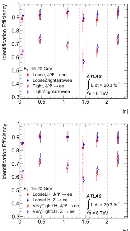
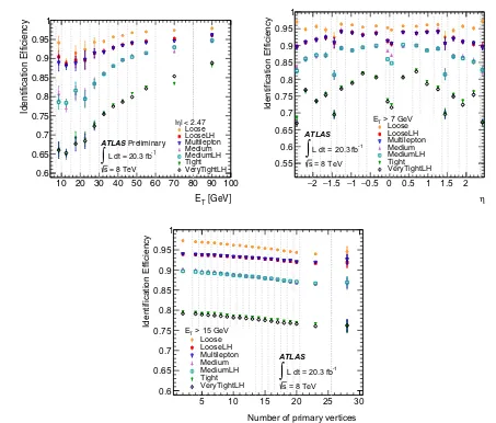
7.4 Results . . . 16
8 Identification efficiency for background processes . 19 8.1 Background efficiency from Monte Carlo sim-ulation . . . 19
8.2 Background efficiency ratios measured from collision data. . . 22
9 Determination of the charge misidentification probability 23 10 Reconstruction efficiency measurement. . . 25
10.1 Tag-and-probe withZ→eeevents . . . 25
10.1.1 Event selection . . . 25
10.1.2 Background estimation and variations for assessing the systematic uncertainties 25 10.2 Results . . . 26
11 Combined reconstruction and identification efficiencies 28 12 Summary . . . 28
References. . . 31
1 Introduction
matched to a track in the inner detector (ID). Electrons are distinguished from other particles using identification crite-ria with different levels of background rejection and signal efficiency. The identification criteria rely on the shapes of EM showers in the calorimeter as well as on tracking quantities and the quality of the matching of the tracks to the clustered energy deposits in the calorimeter. They are based either on independent requirements or on a single requirement, the output of a likelihood function built from these quantities.
In this document, measurements of the efficiency to recon-struct and identify prompt electrons and their EM charge in the central region of the ATLAS detector1with pseudorapid-ity|η|<2.47 are presented forppcollision data produced by the Large Hadron Collider (LHC) in 2012 at a centre-of-mass energy of√s = 8 TeV, and compared to the prediction from Monte Carlo (MC) simulation. The goal is to extract correc-tion factors and their uncertainties for measurements of final states with prompt electrons in order to adjust the MC effi-ciencies to those measured in data. Electrons from semilep-tonic heavy-flavour decays are treated as background.
The efficiency measurements follow the methods intro-duced in Ref. [2] for the 2011 ATLAS electron performance studies but are improved in several respects and adjusted for the 2012 data-taking conditions. The measurements are based on the tag-and-probe method using theZand theJ/ψ
resonances, requiring the presence of an isolated identified electron as thetag. Additional selection criteria are applied to obtain a high purity sample of electron candidates that can be used asprobesto measure the reconstruction or identification efficiency. The measurements span different but overlapping kinematic regions and are studied as a function of the elec-tron’s transverse momentum and pseudorapidity. The results are combined taking into account bin-to-bin correlations.
After briefly describing the ATLAS detector in Sect.2, the algorithms to reconstruct and identify electrons are sum-marized in Sects.3and4. The general methodology of tag-and-probe efficiency measurements and the decomposition of the efficiency into its different components are reviewed in Sect.5. The data and MC samples used in this work are summarized in Sect.6. Sections7and8describe the identi-fication efficiency measurements for signal electrons as well as backgrounds. In Sect.9, the measurement of the electron charge misidentification rate is presented. Section10details the reconstruction efficiency measurement, which extends
1 ATLAS uses a right-handed coordinate system with its origin at the nominalppinteraction point at the centre of the detector. The positive x-axis is defined by the direction from the interaction point to the centre of the LHC ring, with the positivey-axis pointing upwards, while the beam direction defines thez-axis. The azimuthal angleφis measured around the beam axis and the polar angleθis the angle from thez-axis. The pseudorapidity is defined asη= −ln tan(θ/2). The radial distance between two objects is defined asR=
(η)2+(φ)2. Transverse energy is computed asET=E·sinθ.
the identification measurement methodology, and Sect.11 describes the final results of the combined identification and reconstruction efficiency measurements. Section12 con-cludes with a summary of the results.
2 The ATLAS detector
A complete description of the ATLAS detector is provided in Ref. [1]. A brief description of the subdetectors that are relevant for the detection of electrons is given in this section. The ID provides precise reconstruction of tracks within |η|<2.5. It consists of three layers of pixel detectors close to the beam-pipe, four layers of silicon microstrip detector modules with pairs of single-sided sensors glued back-to-back (SCT) providing eight hits per track at intermediate radii, and a transition radiation tracker (TRT) at the outer radii, providing on average 35 hits per track in the range |η|<2.0. The TRT offers substantial discriminating power between electrons and charged hadrons between energies of 0.5 and 100 GeV, via the detection of X-rays produced by transition radiation. The innermost pixel layer in 2012 and earlier, also called the b-layer, is located outside the beam-pipe at a radius of 50 mm. Together with the other layers, it provides precise vertexing and significant rejection of photon conversions through the requirement that a track has a hit in this layer.
The ID is surrounded by a thin superconducting solenoid with a length of 5.3 m and diameter of 2.5 m. The solenoid provides a 2 T magnetic field for the measurement of the curvature of charged particles to determine their charge and momentum. The solenoid design attempts to minimize the amount of material by integrating it into a vacuum vessel shared with the LAr calorimeter. The magnet thus only con-tributes a total of 0.66 radiation lengths of material at normal incidence.
transition region between the EMB and EMEC calorimeters, 1.37<|η|<1.52, suffers from a large amount of material.
Hadronic calorimeters with at least three segments lon-gitudinal in shower depth surround the EM calorimeter and are used in this context to reject hadronic jets. The forward calorimeters cover the range 3.1<|η|<4.9 and also have EM shower identification capabilities given their fine lateral granularity and longitudinal segmentation into three layers.
3 Electron reconstruction
Electron reconstruction in the central region of the ATLAS detector (|η|<2.47) starts from energy deposits (clusters) in the EM calorimeter which are then matched to reconstructed tracks of charged particles in the ID.
3.1 Electron seed-cluster reconstruction
Theη–φspace of the EM calorimeter system is divided into a grid of Nη×Nφ =200×256 towers of sizeηtower× φtower=0.025×0.025, corresponding to the granularity of the EM accordion calorimeter middle layer. The energy of the calorimeter cells in all shower-depth layers (the strip, middle and back EM accordion calorimeter layers and for |η| < 1.8 also the presampler detector) is summed to get the tower energy. The energy of a cell which spans several towers is distributed evenly among the towers without taking into account any geometrical weighting.
To reconstruct the EM clusters, seed clusters of tow-ers with total cluster transvtow-erse energy above 2.5 GeV are searched for by a sliding-window algorithm [3]. The win-dow size is 3×5 towers inη–φspace. A duplicate-removal algorithm is applied to nearby seed clusters.
Cluster reconstruction is expected to be very efficient for true electrons. In MC samples passing the full ATLAS sim-ulation chain, the efficiency is about 95% for electrons with a transverse energy of ET = 7 GeV and reaches 99% at
ET = 15 GeV and 99.9% at ET = 45 GeV, placing a requirement only on the angular distance between the gen-erated electron and the reconstructed electron cluster. The efficiency decreases with increasing pseudorapidity in the endcap region|η|>1.37.
3.2 Electron-track candidate reconstruction
Track reconstruction for electrons was improved for the 2012 data-taking period with respect to the one used for 2011 data-taking, especially for electrons which undergo signif-icant energy loss due to bremsstrahlung in the detector, to achieve a high and uniform efficiency.
Table1shows the definition of shower-shape and track-quality variables, includingRηandRHad. For each seed EM
cluster2passing loose shower-shape requirements of Rη >
0.65 andRHad<0.1 a region-of-interest (ROI) is defined as a cone of sizeR= 0.3 around the seed cluster barycentre. The collection of these EM cluster ROIs is retained for use in the track reconstruction.
Track reconstruction proceeds in two steps: pattern recog-nition and track fit. In 2012, in addition to the standard track-pattern recognition and track fit, an electron-specific track-pattern recognition and track fit were introduced in order to recover losses from bremsstrahlung and therefore improve the recon-struction of electrons. Either of these algorithms, the pattern recognition and the track fit, use a particle-specific hypoth-esis for the particle mass and respective probability for the particle to undergo bremsstrahlung, referred to in the follow-ing either as pion or electron hypothesis.
The standard pattern recognition [4] uses the pion hypoth-esis for energy loss in the material of the detector. If a track3 seed (consisting of three hits in different layers of the silicon detectors) with a transverse momentum larger than 1 GeV cannot be successfully extended to a full track with at least seven hits using the pion hypothesis and it falls within one of the EM cluster ROIs, it is retried with the new pattern recognition using an electron hypothesis that allows for energy loss. This modified pattern recognition algorithm (based on a Kalman filter–smoother formalism [5]) allows up to 30% energy loss at each material surface to account for bremsstrahlung. Below 1 GeV, no refitting is performed. Thus, an electron-specific algorithm has been integrated into the standard track reconstruction; it improves the perfor-mance for electrons and has minimal interference with the main track reconstruction.
Track candidates are fitted using either the pion or the electron hypothesis (according to the hypothesis used in the pattern recognition) with the ATLAS Globalχ2Track Fit-ter [6]. The electron hypothesis employs the same track fit as for the pion hypothesis except that it adds an extra term to compensate for the increase inχ2due to bremsstrahlung losses, in order to be able to fit the track with an acceptableχ2 such that it can be further used in the electron reconstruction. If a track candidate fails the pion hypothesis track fit due to a largeχ2(for example caused by large energy losses), it is refitted using the electron hypothesis.
Tracks are then considered as loosely matched to an EM cluster, if they pass either of the following two requirements:
2 As in the 2011 electron reconstruction algorithm, clusters must satisfy loose requirements on the maximum fraction of energy deposited in the different layers of the EM calorimeter system: 0.9, 0.8, 0.98, 0.8 for the presampler detector, the strip, the middle and the back EM accordion calorimeter layers, respectively.
(i) Tracks with at least four silicon hits are extrapolated from their measured perigee to the middle layer of the EM accordion calorimeter. In the middle layer of the calorimeter, the extrapolated tracks have to be either within 0.2 inφof the EM cluster on the side the track is bending towards or within 0.05 on the opposite side. They also have to be within 0.05 inηof the EM cluster. TRT-only tracks, i.e. tracks with less than four silicon hits, are extrapolated from the last measurement point. They are retained at this early stage as they are used later in the reconstruction chain to reconstruct photon conversions. Clusters without any associated tracks with silicon hits are eventually considered as photons and are not used to reconstruct prompt-electron candidates. TRT-only tracks have to pass the same requirement for the difference inφ between track and cluster as tracks with silicon hits but no requirement is placed on the difference inηbetween track and cluster at this stage as theirηcoordinate is not measured precisely.
(ii) The track extrapolated to the middle layer of the EM accordion calorimeter, after rescaling its momentum to the measured cluster energy, has to be either within 0.1 in φ of the EM cluster on the side the track is bend-ing towards or within 0.05 on the opposite side. Further-more, non-TRT-only tracks must be within 0.05 inηof the calorimeter cluster. As in (i), the track extrapolation is made from the last measurement point for TRT-only tracks and from the point of closest approach with respect to the primary collision vertex for tracks with silicon hits.
Criterion (ii) aims to recover tracks of typically large cur-vature that have potentially suffered significant energy loss before reaching the calorimeter. Rescaling the momentum of the track to that of the reconstructed cluster allows reten-tion of tracks whose measured momentum in the ID does not match the energy reconstructed in the calorimeter because they have undergone bremsstrahlung. The bremsstrahlung is assumed to have occurred in the ID or the cryostat and solenoid before the calorimeter (for tracks with silicon hits) or in the cryostat and solenoid before the calorimeter (for TRT-only tracks).
At this point, all electron-track candidates are defined. The track parameters of these candidates, for all but the TRT-only tracks, are precisely re-estimated using an optimized electron track fitter, the Gaussian Sum Filter (GSF) [7] algo-rithm, which is a non-linear generalization of the Kalman filter [5] algorithm. It yields a better estimate of the electron track parameters, especially those in the transverse plane, by accounting for non-linear bremsstrahlung effects. TRT-only tracks and the very rare tracks (about 0.01%) that fail the GSF fit keep the parameters from the Globalχ2Track Fit. These tracks are then used to perform the final track-cluster
matching to build electron candidates and also to provide information for particle identification.
3.3 Electron-candidate reconstruction
An electron is reconstructed if at least one track is matched to the seed cluster. The efficiency of this matching and sub-sequent track quality requirements is measured as the recon-struction efficiency in Sect.10. The track-cluster matching proceeds as described for the previous step in Sect.3.2, but with the GSF refitted tracks and tighter requirements: the separation inφmust be less than 0.1 (and not 0.2). Addition-ally, TRT-only tracks must satisfy loose track-cluster match-ing criteria in η and tighter ones in φ: in the TRT barrel |η| <0.35 and in the TRT endcap|η|< 0.02. In both the barrel and the endcaps the requirements are|φ|<0.03 on the side the track is bending towards and|φ|<0.02 on the other side. In this procedure, more than one track can be associated with a cluster.
Although all tracks assigned to a cluster are kept for fur-ther analysis, the best-matched one is chosen as the pri-mary track which is used to determine the kinematics and charge of the electron and to calculate the electron identifi-cation decision. Thus choosing the primary track is a crucial step in the electron reconstruction chain. To favour the pri-mary electron track and to avoid random matches between nearby tracks in the case of cascades due to bremsstrahlung, tracks with at least one hit in the pixel detector are pre-ferred. If more than one associated track has pixel hits, the following sorting criteria are considered. First, the distance between the track and the cluster is considered for any pair of tracks, which are referred to asi and j in the following. Then two angular distance variables are defined in the η– φ plane. R is the distance between the cluster barycen-tre and the extrapolated track in the middle layer of the EM accordion calorimeter, whileRrescaled is the distance between the cluster barycentre and the extrapolated track when the track momentum is rescaled to the measured clus-ter energy before the extrapolation to the middle layer. If |Rrescaled,i−Rrescaled,j|>0.01, the track with the smaller
Rrescaledis chosen. If|Rrescaled,i−Rrescaled,j| ≤0.01
and |Ri −Rj| > 0.01, the track with smaller R is
taken. For the rest of the cases, the two tracks have both sim-ilarRrescaledand similarR, and the track with more pixel hits4is chosen as the primary track. A hit in the first layer of the pixel detector counts twice to prefer tracks with early hits. If there are two best tracks with exactly the same numbers of hits, the track with smallerRis taken.
All seed clusters together with their matching tracks, if there is at least one of them, are treated as electron candidates. Each of these electron clusters is then rebuilt in all four layers sequentially, starting from the middle layer, using 3×7 (5×5) cells inη×φin the barrel (endcaps) of the EM accordion calorimeter. The cluster position is adjusted in each layer to take into account the distribution of the deposited energy. The fixed sizes of 3×7 (5×5) cells for electron clusters were optimized to take into account the different overall energy distributions in the barrel (endcap) accordion calorimeters specifically for electrons.5
Up to this point, neither the electron clusters nor the cells inside the clusters are calibrated. The energy calibration [8] is applied as the next step and was improved for 2012 data using multivariate analysis (MVA) techniques [9] and an improved description of the detector [10] by theGEANT4[11] simula-tion. The calibration procedure is outlined briefly below.
After applying the electronic readout calibration to the calorimeter cells with a global energy scale factor corre-sponding to the electron response, a number of data pre-corrections are applied for measured effects of the bunch train structure and imperfectly corrected response in specific regions. The presampler energy scales and the EM accordion calorimeter strip-to-middle-layer energy-scale ratios are also corrected [8].
The cluster energy is then determined from the energy in the three layers of the EM accordion calorimeter by applying a correction factor determined by linear regression using an MVA trained on large samples of single-electron MC events produced with the full ATLAS simulation chain. The input quantities used for electrons and photons are the total energy measured in the accordion calorimeter, the ratio of the energy measured in the presampler to the energy measured in the accordion, the shower depth,6the pseudorapidity of the clus-ter barycentre in the ATLAS coordinate system, and theηand φpositions of the cluster barycentre in the local coordinate system of the calorimeter. Including the cluster barycentre position allows a correction to be made for the larger lateral energy leakage for particles that hit a cell close to the edge and for the variation of the response as a function of the par-ticle impact point with respect to the calorimeter absorbers. In the last step, correction factors are derived in situ using a large sample of collectedZ→eeevents. They are applied to the reconstructed electrons as a final energy calibration in data events. Electron energies are smeared in simulated
5Unconverted (converted) photon clusters, which are used in the recon-struction efficiency measurement in Sect.10, are built using 3×5 (3×7) cells in the barrel and 5×5 (5×5) cells in the endcap.
6The shower depth is defined asX=
iXiEi/iEiwhereEiis the cluster energy in layeriandXiis the approximate calorimeter thickness (in radiation lengths) from the interaction point to the middle of layer i, including the presampler detector layer where present.
events, as the simulated electrons have a better energy reso-lution than electrons in data.
The four-momentum of central electrons (|η|<2.47) is computed using information from both the final cluster and the track best matched to the original seed cluster. The energy is given by the cluster energy. The φandη directions are taken from the corresponding track parameters, except for TRT-only tracks for which the cluster φ andη values are used.
4 Electron identification
Not all objects built by the electron reconstruction algorithms are prompt electrons which are considered signal objects in this publication. Background objects include hadronic jets as well as electrons from photon conversions, Dalitz decays and from semileptonic heavy-flavour hadron decays. In order to reject as much of these backgrounds as possible while keep-ing the efficiency for prompt electrons high, electron iden-tification algorithms are based on discriminating variables, which are combined into a menu of selections with various background rejection powers. Sequential requirements and MVA techniques are employed.
Variables describing the longitudinal and lateral shapes of the EM showers in the calorimeters, the properties of the tracks in the ID, as well as the matching between tracks and energy clusters are used to discriminate against the different background sources. These variables [2,12,13] are detailed in Table 1. Table 2 summarizes which variables are used for the different selections of the so-called cut-based and likelihood (LH) [14] identification menus.
4.1 Cut-based identification
The cut-based selections, Loose, Medium, Tight and Multi-lepton, are optimized in 10 bins in|η|and 11 bins inET. This binning allows the identification to take into account the vari-ation of the electrons’ characteristics due to e.g. the depen-dence of the shower shapes on the amount of passive mate-rial traversed before entering the EM calorimeter. Shower shapes and track properties also change with the energy of the particle. The electrons selected with Tight are a subset of the electrons selected with Medium, which in turn are a subset of Loose electrons. With increasing tightness, more variables are added and requirements are tightened on the variables already used in the looser selections.
Table 1 Definition of electron discriminating variables
Type Description Name
Hadronic leakage Ratio ofETin the first layer of the hadronic calorimeter toETof the EM cluster (used over the range|η|<0.8 or|η|>1.37)
RHad1
Ratio ofETin the hadronic calorimeter toETof the EM cluster (used over the range 0.8<|η|<1.37)
RHad
Back layer of EM calorimeter Ratio of the energy in the back layer to the total energy in the EM accordion calorimeter f3 Middle layer of EM calorimeter Lateral shower width,
(Eiηi2)/(Ei)−((Eiηi)/(Ei))2, whereEiis the energy andηiis the pseudorapidity of celliand the sum is calculated within a window of 3×5 cells
wη2
Ratio of the energy in 3×3 cells to the energy in 3×7 cells centred at the electron cluster position
Rφ
Ratio of the energy in 3×7 cells to the energy in 7×7 cells centred at the electron cluster position
Rη
Strip layer of EM calorimeter Shower width,(Ei(i−imax)2)/(Ei), whereiruns over all strips in a window of
η×φ≈0.0625×0.2, corresponding typically to 20 strips inη, andimaxis the index of the highest-energy strip
wstot
Ratio of the energy difference between the maximum energy deposit and the energy deposit in a secondary maximum in the cluster to the sum of these energies
Eratio
Ratio of the energy in the strip layer to the total energy in the EM accordion calorimeter f1 Track quality Number of hits in the b-layer (discriminates against photon conversions) nBlayer
Number of hits in the pixel detector nPixel
Total number of hits in the pixel and SCT detectors nSi
Transverse impact parameter d0
Significance of transverse impact parameter defined as the ratio of the magnitude ofd0 to its uncertainty
σd0
Momentum lost by the track between the perigee and the last measurement point divided by the original momentum
p/p
TRT Total number of hits in the TRT nTRT
Ratio of the number of high-threshold hits to the total number of hits in the TRT FHT Track-cluster matching ηbetween the cluster position in the strip layer and the extrapolated track η
φbetween the cluster position in the middle layer and the extrapolated track φ Defined asφ, but the track momentum is rescaled to the cluster energy before
extrapolating the track to the middle layer of the calorimeter
φres
Ratio of the cluster energy to the track momentum E/p Conversions Veto electron candidates matched to reconstructed photon conversions isConv
improved by loosening requirements and introducing addi-tional variables, especially in the looser selections [2]. In 2012, for√s=8 TeV collisions, due to higher instantaneous luminosities provided by the LHC, the number of overlap-ping collisions (pile-up) and therefore the number of particles in an event7increased. Due to the higher energy density per event, the shower shapes, even of isolated electrons, tend to look more background-like. In order to cope with this, requirements were loosened on the variables most sensitive to pile-up (RHad(1)andRη) and tightened on others to keep the performance (efficiency/background rejection) roughly constant as a function of the number of reconstructed
pri-7Here an “event” refers to a triggered bunch crossing with all its hard and softppinteractions, as recorded by the detector.
mary vertices. A requirement on f3was added in 2012, as well. Furthermore, a new selection was added, called Multi-lepton, which is optimized for the low-energy electrons in the
H → Z Z∗ →4(=e, μ) analysis. For these electrons, Multilepton has a similar efficiency to the Loose selection, but provides a better background rejection. In comparison to Loose, requirements on the shower shapes are loosened and more variables are added, including those sensitive to bremsstrahlung effects.
4.2 Likelihood identification
Table 2 The variables used in the different selections of the electron identification menu
Cut-based Likelihood
Name Loose Medium Tight Multilepton Loose LH Medium LH Very Tight LH
RHad(1)
f3
wη2
Rη
Rφ
wstot
Eratio
f1
nBlayer
nPixel
nSi
d0
σd0
p/p
nTRT
FHT
η
φ
φres
E/p
isConv
was chosen for electron identification because of its simple construction.
The electron LH makes use of signal and background probability density functions (pdfs) of the discriminating variables. Based on these pdfs, which are treated as uncor-related, an overall probability is calculated for the object to be signal or background. The signal and background prob-abilities for a given electron candidate are combined into a discriminantdL:
dL= LS
LS+LB, L
S(B)(x)=
n
i=1
PS(B),i(xi) (1)
wherexis the vector of variable values and PS,i(xi)is the
value of the signal probability density function of theith variable evaluated atxi. In the same way,PB,i(xi)refers to
the background probability density function.
Signal and background pdfs used for the electron LH iden-tification are obtained from data. As in the Multilepton cut-based selection, variables sensitive to bremsstrahlung effects are included.
Furthermore, additional variables with significant dis-criminating power but also a large overlap between signal and background that prevents explicit requirements (likeRφ
and f1) are included. The variables counting the hits on the track are not used as pdfs in the LH, but are left as simple
requirements, as every electron should have a high-quality track to allow a robust momentum measurement.
The Loose LH, Medium LH, and Very Tight LH selections are designed to roughly match the electron efficiencies of the Multilepton, Medium and Tight cut-based selections, but to have better rejection of light-flavour jets and conversions.8
Each LH selection places a requirement on a LH dis-criminant, made with a different set of variables. The Loose LH features variables most useful for discrimination against light-flavour jets (in addition, a requirement on nBlayer is applied to reject conversions). In the Medium LH and Very Tight LH regimes, additional variables (d0, isConv) are added for further rejection of heavy-flavour jets and conversions. Although different variables are used for the different selec-tions, a sample of electrons selected using a tighter LH is a subset of the electron samples selected using the looser LH to a very good approximation.
The LH for each selection consists of 9×6 sets of pdfs, divided into 9|η|bins and 6ETbins. This binning is similar to, but coarser than, the binning used for the cut-based
tions. It is chosen to balance the available number of events with the variation of the pdf shapes inETand|η|.
4.3 Electron isolation
In order to further reject hadronic jets misidentified as elec-trons, most analyses require electrons to pass some isolation requirement in addition to the identification requirements described above. The two main isolation variables are:
• Calorimeter-based isolation:
The calorimetric isolation variableETconeRis defined as the sum of the transverse energy deposited in the calorimeter cells in a cone of sizeRaround the electron, excluding the contribution withinη×φ =0.125×0.175 around the electron cluster barycentre. It is corrected for energy leak-age from the electron shower into the isolation cone and for the effect of pile-up using a correction parameterized as a function of the number of reconstructed primary vertices.
• Track-based isolation:
The track isolation variable pconeT R is the scalar sum of the transverse momentum of the tracks withpT>0.4 GeV in a cone ofR around the electron, excluding the track of the electron itself. The tracks considered in the sum must originate from the primary vertex associated with the electron track and be of good quality; i.e. they must have at least nine silicon hits, one of which must be in the innermost pixel layer. Both types of isolation are used in the tag-and-probe mea-surements, mainly in order to tighten the selection criteria of the tag. Whenever isolation is applied to the probe electron candidate in this work (this only happens in theJ/ψanalysis described in Sect.7.2), the criteria are chosen such that the effect on the measured identification efficiency is estimated to be small.
5 Efficiency measurement methodology
5.1 The tag-and-probe method
Measuring the identification and reconstruction efficiency requires a clean and unbiased sample of electrons. The method of choice is the tag-and-probe method, which makes use of the characteristic signatures ofZ→eeandJ/ψ→ee
decays. In both cases, strict selection criteria are applied on one of the two decay electrons, called tag, and the second electron, the probe, is used for the efficiency measurements. Additional event selection criteria are applied to further reject background. Only events satisfying data-quality criteria, in particular concerning the ID and the calorimeters, are
consid-ered. Furthermore, at least one reconstructed primary vertex with at least three tracks must be present in the event. The tag-and-probe pairs must also pass requirements on their recon-structed invariant mass. In order to not bias the selected probe sample, each valid combination of electron pairs in the event is considered; an electron can be the tag in one pair and the probe in another.
The probe samples are contaminated by background objects (for example, hadrons misidentified as electrons, electrons from semileptonic heavy flavour decays or from photon conversions). This contamination is estimated using either background template shapes or combined fits of back-ground and signal analytical models to the data. The number of electrons is independently estimated at the probe level and at the level where the probe electron candidate satisfies the tested criteria. The efficiencyis defined as the fraction of probe electrons satisfying the tested criteria.
The efficiency to detect an electron is divided into differ-ent compondiffer-ents, namely trigger, reconstruction and iddiffer-entifi- identifi-cation efficiencies, as well as the efficiency to satisfy addi-tional analysis criteria, like isolation. The full efficiencytotal for a single electron can be written as:
total=reconstruction×identification×trigger×additional
= Nreconstruction
Nclusters ×
Nidentification
Nreconstruction
× Ntrigger
Nidentification ×
Nadditional
Ntrigger .
(2)
The efficiency components are defined and measured in a specific order to preserve consistency: the reconstruction efficiency, reconstruction, is measured with respect to elec-tron clusters reconstructed in the EM calorimeter Nclusters; the identification efficiencyidentificationis determined with respect to reconstructed electronsNreconstruction. Trigger effi-ciencies are calculated for reconstructed electrons satisfying a given identification criterion Nidentification. Therefore, for each identification selection a dedicated set of trigger effi-ciency measurements is performed. Additional selection cri-teria are often imposed in analyses of collision data, for exam-ple on the isolation of electrons (introduced in Sect.4.3). Nei-ther trigger nor isolation efficiency measurements are cov-ered here.
from converted photons that are radiated off an electron orig-inating from a Z or J/ψ decay are also accepted by the analyses. The denominator of the reconstruction efficiency includes electrons that were not properly reconstructed. If electrons in the simulatedZ→eesamples are reconstructed as clusters without a matching track, theZ decay electrons provided by the MC simulation are matched to the recon-structed cluster withinR<0.2.
5.1.1 Data-to-MC correction factors
The accuracy with which the MC detector simulation mod-els the electron efficiency plays an important role in cross-section measurements and various searches for new physics. In order to achieve reliable results, the simulated MC samples need to be corrected to reproduce the measured data efficien-cies as closely as possible. This is achieved by a multiplica-tive correction factor defined as the ratio of the efficiency measured in data to that in the simulation. These data-to-MC correction factors are usually close to unity. Deviations come from the mismodelling of tracking properties or shower shapes in the calorimeters.
Since the electron efficiencies depend on the transverse energy and pseudorapidity, the measurements are performed in two-dimensional bins in (ET,η). These bins follow the detector geometry and the binning used for optimization and are as narrow as the size of the respective data set allows. Residual effects, due to the finite bin widths and kinematic differences of the physics processes used in the measure-ments, are expected to cancel in the data-to-MC efficiency ratio. Therefore, the combination of the different efficiency measurements is carried out using the data-to-MC ratios instead of the efficiencies themselves. The procedure for the combination is described in Sect.7.3.
5.2 Determination of central values and uncertainties
For the evaluation of the results of the measurements and their uncertainties using a given final state (Z→ee,Z →eeγor
J/ψ→ee), the following approach was chosen. The details of the efficiency measurement methods are varied in order to estimate the impact of the analysis choices and poten-tial imperfections in the background modelling. Examples of these variations are the selection of the tag electron or the background estimation method. For the measurement of the data-to-MC correction factors, the same variations of the selection are applied consistently in data and MC simulation. Uncertainties due to charge misidentification of the tag-and-probe pairs are neglected.
The final result (the central value) of a given efficiency measurement using one of theZ→ee,Z →eeγorJ/ψ→ eeprocesses is taken to be the average value of the results from all variations (including the use of different background
subtraction methods, e.g.ZisoandZmassfor theZ→eefinal state as described in Sects.7.1.2,7.1.3).
The systematic uncertainty is estimated to be equal to the root mean square (RMS) of the measurements with the inten-tion of modelling a 68% confidence interval. However, in many bins the RMS does not cover at least 68% of all the variations, so an empirical factor of 1.2 is applied to the deter-mined uncertainty in all bins.
The statistical uncertainty is taken to be the average of the statistical uncertainties over all investigated variations of the measurement. The statistical uncertainty in a single variation of the measurement is calculated following the approach in Ref. [15].
6 Data and Monte Carlo samples
The results in this paper are based on 8 TeV LHC pp colli-sion data collected with the ATLAS detector in 2012. After requiring good data quality, in particular concerning the ID and the EM and hadronic calorimeters, the integrated lumi-nosity used for the measurements is 20.3 fb−1.
The measurements are compared to predictions from MC simulation. TheZ→eeandZ →eeγMC samples are gen-erated with thePOWHEG-BOX[16–18] generator interfaced toPYTHIA8[19], using theCT10NLO PDF set [20] for the hard process, the CTEQ6L1PDF set [21] and a set of tuned parameters called theAU2CT10showering tune [22] for the parton shower. The J/ψ→eeevents are simulated usingPYTHIA8both for prompt (pp→ J/ψ+X) and for non-prompt (bb¯ → J/ψ+X) production. TheCTEQ6L1
LO PDF set is used, as well as theAU2CTEQ6L1parameter set for the showering [22]. All MC samples are processed through the full ATLAS detector simulation [10] based on
GEANT4[11].
The distribution of material in front of the presampler detector and the EM accordion calorimeter as a function of |η|is shown in the left plot of Fig.1. The contributions of the different detector elements up to the ID boundaries, includ-ing services and thermal enclosures, are detailed on the right. These material distributions are used as input to the MC sim-ulation.
The peak at|η| ≈1.5 in the left plot of Fig.1, correspond-ing to the transition region between the barrel and endcap EM accordion calorimeters, is due to the cryostats, the corner of the barrel EM accordion calorimeter, the ID services and parts of the scintillator-tile hadronic calorimeter. The sud-den increase of material at|η| ≈3.2, corresponding to the transition between the endcap calorimeters and the forward calorimeter, is mostly due to the cryostat that acts also as a support structure.
| η | 0 0.5 1 1.5 2 2.5 3 3.5 4 4.5 5 ]0
Radiation length [X
0 2 4 6 8 10 12 14 16
before calorimeter
0
X
before presampler
0
X ATLAS
Simulation
| η | 0 0.5 1 1.5 2 2.5 3 3.5 4 4.5 5 ] 0
Radiation length [X
0 0.5 1 1.5 2
2.5 Services
TRT SCT Pixel Beam-pipe ATLAS
Simulation
Fig. 1 Amount of material, in units of radiation lengthX0, traversed by a particle as a function of|η|: material in front of the presampler detec-tor and the EM accordion calorimeter (left), and material up to the ID
boundaries (right). The contributions of the different detector elements, including the services and thermal enclosures are shown separately by filled colour areas
Fraction
0.02 0.04 0.06 0.08 0.1 0.12 0.14 0.16 0.18 0.2 0.22
ATLAS
ee Data → Z
= 8 TeV
s ∫L dt = 20.3 fb-1
< 30 GeV T 15 GeV < E
< 50 GeV T 30 GeV < E
Number of reconstructed primary vertices
5 10 15 20 25
Ratio
0.5 1 1.5
Fig. 2 Number of reconstructed primary vertices in events with an electron cluster candidate with 15 GeV<ET<30 GeV (open circles) and 30 GeV<ET<50 GeV (filled squares) in the Z→ee data set used for the reconstruction efficiency measurement described in Sect.10
and subsequent bunch crossings. The energies of the elec-tron candidates in simulation are smeared to match the res-olution in data and the simulated MC events are weighted to reproduce the distributions of the primary-vertexz-position and the number of vertices in data, the latter being a good indicator of pile-up. Figure 2 shows the distribution of the number of primary collision vertices in events with an identified electron and an electron cluster candidate (with 15 GeV< ET <30 GeV and 30 GeV< ET <50 GeV) in theZ→eedata set used for the reconstruction efficiency measurement described in Sect.10. The distribution does not depend on the transverse energy of the cluster of the probe electron candidate.
7 Identification efficiency measurement
The efficiencies of the identification criteria (Loose, Medium, Tight, Multilepton and Loose LH, Medium LH, Very Tight LH) are determined in data and in the simulated samples with respect to reconstructed electrons with associated tracks that have at least one hit in the pixel detector and at least seven total hits in the pixel and SCT detectors (this requirement is referred to as “track quality” below). The efficiencies are calculated as the ratio of the number of electrons passing a certain identification selection (numerator) to the number of electrons with a matching track satisfying the track quality requirements (denominator).
For the identification efficiencies determined in this paper, three different decays of resonances are used, and com-bined in the overlapping regions as described in Sect. 7.3: radiative decays of the Z boson, Z → eeγ, for elec-trons with 10 GeV< ET<15 GeV, Z→eefor electrons with ET > 15 GeV and J/ψ → ee for electrons with 7 GeV<ET<20 GeV. The distributions of the probe elec-tron candidates passing the Tight identification selection are depicted in Fig.3as a function ofη(left) andET(right), giv-ing an indication of the number of events available for each of the measurements in the respectiveηandETbin. TheET spectrum of probe electron candidates from J/ψ → eeis discontinuous, as the sample is selected by a number of trig-gers with differentETthresholds as discussed in Sect.7.2.
7.1 Tag-and-probe withZ→eeevents
[image:10.595.308.544.56.210.2] [image:10.595.53.287.283.463.2]η
2.5
− −2 −1.5 −1 −0.5 0 0.5 1 1.5 2 2.5
Entries / 0.1
2 10
3 10
4 10
5 10
6 10
7
10 ZJ/→ψ→ ee ee
γ ee → Z ATLAS
= 8 TeV s
∫
L dt = 20.3 fb-1[GeV] T E
0 10 20 30 40 50 60 70 80 90 100
Entries / GeV
3 10
4 10
5 10
6 10
7 10
ee → Z
ee → ψ J/
γ ee → Z ATLAS
= 8 TeV s
∫
L dt = 20.3 fb-1Fig. 3 Pseudorapidity and transverse energy distributions of probe electron candidates satisfying the Tight identification criterion in the
Z→ee(full circles),Z →eeγ (empty triangles) and theJ/ψ→ee
(full triangles) samples. TheETdistribution of probe electron
candi-dates fromJ/ψ→eeis discontinuous, as the sample is selected by a number of triggers with differentETthresholds
ET >25 GeV. For lower transverse energies, background subtraction becomes important. Two different distributions are used to discriminate signal electrons from background: the invariant mass of the tag-and-probe pair is used in the
Zmassmethod and the isolation distribution of the probe elec-tron candidate is used in theZisomethod.
Probe electrons withETbetween 10 GeV and 15 GeV are selected fromZ→eeγdecays in which an electron has lost much of its energy due to final-state radiation (FSR). At low
ET, this topology has less background thanZ→eedecays. The invariant mass in these cases is computed from three objects: the tag electron, the probe electron and a photon.
7.1.1 Event selection
Events are selected using a logical OR between two single-electron triggers, one with anETthreshold of 24 GeV requir-ing medium identification and one with anETthreshold of 60 GeV and loose identification requirements.9
Events are required to have at least two reconstructed electron candidates in the central region of the detector, |η|<2.47, with opposite charges (see Sect.9for the measure-ment of the charge misidentification). The tag electron can-didate is required to have a transverse energyET>25 GeV, be matched to a trigger electron within R < 0.15 and be outside the transition region between barrel and endcap of the EM calorimeter, 1.37<|η|<1.52. Furthermore, it has to pass the Tight identification requirement (Medium for Z → eeγ). The probe electron candidates must have
ET>10 GeV and satisfy the track quality criteria. The invari-ant mass of the tag–probe (tag–probe–photon forZ →eeγ)
9The electron identification selection in the trigger is looser than or equivalent to the corresponding analysis requirements.
system is required to be within ±15 GeV of the Z mass. About 15.5 million probe electron candidates are selected for further analysis.
For the Z → eeγ method, in addition to the tag and the probe electron candidates, a photon is selected pass-ing Tight photon identification requirement [23] and ful-filling ET(probe) + ET(photon) >30 GeV. Requirements are placed on the angular distance between the photon and the electron candidates to avoid double counting of objects: R(tag–photon)>0.4 andR(probe–photon)>0.2. The reason for the asymmetry between tag and probe electron requirements is an isolation requirement with a cone size of 0.4 which is applied to the tag electron as one of the varia-tions for assessing the systematic uncertainties. Furthermore, FSR photons from the probe electron tend to be closer to the probe electron than to the tag electron. Further require-ments are placed on the tag–probe and tag–photon invariant mass to select events with FSR:m(tag + photon)<80 GeV,
m(tag + probe)< 90 GeV. All possible tag–probe–photon combinations are used. About 13,000 probe electron candi-dates with a transverse energy of 10 GeV<ET<15 GeV are selected integrated over the full|η|<2.47 range.
7.1.2 Background estimation and variations for assessing the systematic uncertainties of the Zmassmethod
The invariant mass of the tag-and-probe pair (and the photon in the case ofZ →eeγ) is used as the discriminating variable between signal electrons and background.
[image:11.595.305.541.54.229.2][GeV]
ee
m
60 80 100 120 140 160
Entries / GeV
2000 4000 6000 8000
10000 ATLAS
< 25 GeV T
20 GeV < E < 0.6
η
0.1 < = 8 TeV
s
∫
L dt = 20.3 fb-1Data, all probes
Background template
ee MC → Z
Expected (template + MC)
[GeV]
ee
m
60 80 100 120 140 160
Entries / GeV
2000 4000 6000 8000
10000 ATLAS
< 25 GeV T
20 GeV < E < 0.6
η
0.1 < = 8 TeV
s
∫
L dt = 20.3 fb-1Data, Tight probes
Background template
ee MC → Z
Expected (template + MC)
Fig. 4 Illustration of the background estimation using the Zmass method in the 20 GeV<ET<25 GeV, 0.1< η <0.6 bin, at reconstruc-tion + track-quality level (left) and for probe electron candidates passing the cut-based Tight identification (right). The background template is
normalized in the range 120 GeV<mee<250 GeV. The tag electron passes cut-based Medium and isolation requirements. The signal MC simulation is scaled to match the estimated signal in theZ-mass window
[GeV]
γ
ee
m
60 80 100 120 140 160
Entries / GeV
100 200 300 400 500 600
ATLAS
< 15 GeV T
[image:12.595.303.541.283.458.2] [image:12.595.55.289.285.456.2]10 GeV < E | < 0.8
η
0.1 < | = 8 TeV
s
∫
L dt = 20.3 fb-1Data, all probes
Background template
MC γ ee → Z
Expected (template + MC)
[GeV]
γ
ee
m
60 80 100 120 140 160
Entries / GeV
100 200 300 400 500 600
ATLAS
< 15 GeV T
10 GeV < E | < 0.8
η
0.1 < | = 8 TeV
s
∫
L dt = 20.3 fb-1Data, Tight probes
Background template
MC γ ee → Z
Expected (template + MC)
Fig. 5 Illustration of the background estimation using theZ →eeγ method in the 10 GeV<ET<15 GeV, 0.1<|η|<0.8 bin, at recon-struction + track-quality level (left) and for probe electron candidates passing the cut-based Tight identification (right). The background
tem-plate is normalized in the range 100 GeV<mee<250 GeV. The tag electron passes cut-based Medium and isolation requirements. The sig-nal MC simulation is scaled to match the estimated sigsig-nal in theZ-mass window
data and simulated samples to test the shape biases of pos-sible background templates due to the inversion of selection requirements and contamination from signal electrons, and the least-biased templates were chosen. The remaining sig-nal electron contamination in the background templates is estimated using simulated events.
The normalization of the background template is deter-mined by a sideband method: for the denominator (defined at the beginning of Sect. 7), the templates are normal-ized to the invariant-mass distribution above the Z peak (120 GeV < mee < 250 GeV for Z→ee and 100 GeV
<meeγ <250 GeV forZ →eeγ).
Care is taken to remove the small contribution of signal electrons in the tails of the distribution of all probes before normalizing the background template to them. Tight probe
electrons and Tight data efficiencies are used to perform this subtraction, except for the Tight efficiency extraction, for which the MC efficiency is used. For the numerator, the same templates are used as in the denominator, but they are normalized to the same-sign invariant-mass distribution (all numerator requirements are imposed on the probe). The nor-malization is done in the same ranges as in the denominator. The same-sign distribution is used as reference because it has less signal contamination than the opposite-sign distribution, an effect that is more important in the numerator. Figure4 shows theZ→eetag-and-probe invariant-mass distribution in one example bin for both numerator and denominator, including the normalized background template and the MC
Z→eeprediction. Figure5shows the same for theZ →eeγ
[GeV] cone0.3 T E 5
− 0 5 10 15 20 25 30 35
Entries / 8.33 GeV
0 1000 2000 3000 4000
5000 ATLAS
< 20 GeV T
15 GeV < E < -0.1
η
-0.6 < = 8 TeV
s
∫
L dt = 20.3 fb-1Data, all probes
Background template
[GeV] cone0.3 T E 5
− 0 5 10 15 20 25 30 35
Entries / 8.33 GeV
0 1000 2000 3000 4000
5000 ATLAS
< 20 GeV T
15 GeV < E < -0.1
η
-0.6 < = 8 TeV
s
∫
L dt = 20.3 fb-1Data, Tight probes
Background template
Fig. 6 Illustration of the background estimation using theZisomethod in the 15 GeV<ET<20 GeV,−0.6< η <−0.1 bin, at reconstruc-tion + track-quality level (left) and after applying the cut-based Tight
identification (right). The tag electrons are selected using the cut-based Tight identification and aZ-mass window of 15 GeV is applied. The threshold chosen for the sideband subtraction isEcone0.3T =12.5 GeV
In order to assess systematic uncertainties, efficiency mea-surements based on the following variations of the analysis are considered. The mass window is changed from 15 to 10 and 20 GeV around the Z mass, the tag electron require-ment is varied by applying a requirerequire-ment on the calorimet-ric isolation variable and, in theZ→eecase, by loosening the identification requirement to Medium. Furthermore, for
ET<30 GeV, two normalization regions, below and above theZpeak are used. The normalization range below the peak is 60 GeV<mee<70 GeV. ForET>30 GeV, the number of events in the low-mass region is too small for a reliable normalization, so instead two different background template selections are considered. All possible combinations of these variations are produced and taken into account as described in Sect.5.2.
7.1.3 Background estimation and variations for assessing the systematic uncertainties of the Zisomethod
In this approach, the calorimeter isolation distributionETcone0.3
of the probe electron candidates is used as the discriminating variable.
The background templates are formed as subsets of all probe electron candidates used in the denominator of the identification efficiency calculation. The probes for the back-ground template are required to be reconstructed as electrons with a matching track that satisfies track quality criteria; however, they are required to fail some of the identification requirements, namely the requirements onwstotandFHT. A study was performed on possible background templates and the bias due to the inversion of selection requirements and contamination from signal electrons. The least-biased tem-plates were chosen. As illustrated in Fig.6, the background templates are normalized to the isolation distribution of the
probe electron candidates using the background dominated tail region of the isolation distribution.
To assess the systematic uncertainty of the efficiency, the parameters of the measurement are varied. The threshold for the sideband subtraction is chosen betweenEcone0T .3=10 GeV and=15 GeV. As in the Zmass case, the mass window is changed from 15 GeV to 10 GeV and 20 GeV around the
Z mass, the tag electron requirement is varied by apply-ing a requirement on the calorimetric isolation variable,
ETcone0.4<5 GeV.
In addition, different identification requirements are inverted to form two alternative templates and an alternative probe electron isolation distribution ETcone0.4 with a larger isolation cone size (R =0.4) is used as the discriminant. As in theZmasscase, all possible combinations of these vari-ations are considered.
For theZmassandZisomethods together, there are in total 90 variations, which are treated as variations of the same measurement in order to estimate the systematic uncertainty due to the background estimation method.
7.2 Tag-and-probe with J/ψ→eeevents
J/ψ→eeevents are used to measure the electron identifi-cation efficiency for 7 GeV< ET <20 GeV. At such low energies, the probe sample suffers from a significant back-ground fraction, which can be estimated using the recon-structed dielectron invariant mass (mee) of the selected
tag-and-probe pairs. Furthermore, theJ/ψsample is composed of two contributions. In prompt production, the J/ψmeson is produced directly in the proton–proton collision via strong interaction or from the decays of directly produced heavier charmonium states. The electrons from the decay of prompt
[image:13.595.54.291.52.227.2]have identification efficiencies close to those of isolated elec-trons from other physics processes of interest in the same transverse energy range, such as Higgs boson decays. In non-prompt production, theJ/ψmeson originates fromb-hadron decays and its decay electrons are expected to be less isolated. Experimentally, the two production modes can be distin-guished by measuring the displacement of the J/ψ → ee
vertex with respect to the primary vertex. Due to the long lifetime ofb-hadrons, electron-pairs from non-prompt J/ψ
production have a measurably displaced vertex, while prompt decays occur at the primary vertex. To reduce the depen-dence on theJ/ψtransverse momentum, the variable used in this analysis to discriminate between prompt and non-prompt production, called pseudo-proper time [24], is defined as
τ = Lx y·m
J/ψ
PDG
pTJ/ψ . (3)
Here,Lx ymeasures the displacement of theJ/ψvertex with
respect to the primary vertex in the transverse plane, while
mPDGJ/ψ andpTJ/ψare the mass [25] and the reconstructed trans-verse momentum of theJ/ψparticle.
Two methods have been developed to measure the elec-tron efficiency usingJ/ψ→eedecays. The short-τmethod, already used in Refs. [2,13], considers only events with short pseudo-proper time, selecting a subsample dominated by promptJ/ψproduction. The remaining non-prompt contam-ination is estimated using MC simulation and the measure-ment of the non-prompt fraction inJ/ψ→μμevents [26]. Theτ-fit method, used in Ref. [2], utilizes the fullτ-range and extracts the non-prompt fraction by fitting the pseudo-proper time distribution both before and after applying the identification requirements.
7.2.1 Event selection
Events are selected by five dedicated J/ψ → eetriggers. These require tight trigger electron identification10 and an electron ET above a threshold for one of the two trigger objects, while only requiring an EM cluster above a certain
ETthreshold for the other.
Events with at least two electron candidates withET > 5 GeV and|η|<2.47 are considered.
The tag electron candidate must be matched to a tight trig-ger electron object withinR <0.005 and satisfy the cut-based Tight identification selection. To further clean the tag electron sample an isolation criterion is applied in most of the analysis variations. The other electron candidate, the probe, needs to satisfy the track quality criteria. It is also required
10The tight electron identification selection applied in theJ/ψtrigger is looser than the corresponding analysis requirements. In particular, no selection is applied toφ,E/pand isConv.
to match an EM trigger object of the J/ψ → eetriggers withinR <0.005 and have a transverse energy that is at least 1 GeV higher than the corresponding trigger threshold. To ensure that the measured efficiency corresponds to well-isolated electrons an isolation requirement is imposed on the probe electron candidate as well. The isolation criterion has less than 1% effect on the identification efficiency in sim-ulated events. It is further required that the tag and probe electron candidates are separated by Rtag−probe > 0.2 to prevent one electron from affecting the identification of the other. The pseudo-proper time of the reconstructedJ/ψ can-didate is restricted to−1 ps< τ <3 ps in theτ-fit method and typically to−1 ps< τ <0.2 ps in the short-τ method. The negative values of the pseudo-proper times are due to the finite resolution ofLx y. At this stage no requirement is
made on the charge of the electrons and all possible tag-and-probe pairs are considered. About 700,000 tag-and-probe electron candidates are selected forET=7–20 GeV, of which about 190,000 pass the Tight selection, within the range of−1 ps < τ <3 ps and integrated over|η|<2.47.
7.2.2 Background estimation and variations for assessing the systematic uncertainties
The invariant mass of the tag-and-probe pair is used to dis-criminate between signal electrons and background. The most important contribution to the background, even after requiring the tag-and-probe pair to have opposite-sign (OS) charges, comes from random combinations of two parti-cles. This can be evaluated – assuming charge symmetry – using the mass spectrum of same-sign (SS) charge pairs. The remaining background is small and can be described using an analytical model. For this, the invariant-mass distribution of the two electron candidates is fitted with the sum of three contributions:J/ψ,ψ(2S) and background, typically in the range of 1.8 GeV<mee<4.6 GeV. To model theJ/ψ
com-ponent, a Crystal-Ball [27,28] function is used. In theτ-fit method to better describe the tail, a Crystal-Ball + Gaussian function is used instead. Theψ(2S) is modelled with the same shape except for an offset corresponding to the mass differ-ence between theJ/ψandψ(2S) states. Finally the residual background is modelled by a Chebyshev polynomial (as vari-ation by an exponential function) with the parameters deter-mined from a combined signal + background fit to the data. The background estimated using SS pairs is either added to the residual background in the binned fit (see Fig.7for the short-τ method) or subtracted explicitly before performing the unbinned fit (see Fig.8for theτ-fit method). The num-ber of J/ψcandidates is counted within a mass window of 2.8 GeV<mee<3.3 GeV.
[MeV]
ee
m
2000 2500 3000 3500 4000 4500
Entries / 100 MeV
0 100 200 300 400 500 600 700 800 900 ATLAS
< 15 GeV T
[image:15.595.304.542.330.503.2] [image:15.595.54.290.331.502.2]10 GeV < E | < 2.47
η
2.01 < |
= 8 TeV
s
∫
L dt = 20.3 fb-1OS data, all probes
Fit result ee signal → ψ J/ ee signal → (2S) ψ Total background SS data Residual background [MeV] ee m
2000 2500 3000 3500 4000 4500
Entries / 100 MeV
0 100 200 300 400 500 600 ATLAS
< 15 GeV T
10 GeV < E | < 2.47
η
2.01 < |
= 8 TeV
s
∫
L dt = 20.3 fb-1OS data, Tight probes
Fit result ee signal → ψ J/ ee signal → (2S) ψ Total background SS data Residual background
Fig. 7 The figure demonstrates the background subtraction as carried out in the short-τmethod. Shown is the dielectron invariant-mass fit for all probe electron candidates having a good track quality (left) and for probe electron candidates passing the cut-based Tight identification
(right) for 10 GeV<ET<15 GeV and 2.01<|η|<2.47. A track
isolation requirement of pcone0T .2/ET < 0.15 is placed on the probe electron candidate. The pseudo-proper time is required to be−1 ps
< τ <0.2 ps.Dots with error barsrepresent the opposite-sign (OS) pairs for data, the fittedJ/ψsignal is shown by thedashed blueand the
ψ(2S) by thedashed light blue lines(both modelled by a Crystal-Ball function). A background fit is carried out using the sum of the same-sign (SS) distribution (solid grey) from data and a Chebyshev polynomial of 2nd order describing the residual background (dashed grey). The sum of the two background contributions is depicted as apurple dotted line
[MeV]
ee
m
2000 2500 3000 3500 4000 4500
Entries / 100 MeV
0 1000 2000 3000 4000 5000 6000 7000 ATLAS
< 15 GeV T
10 GeV < E | < 0.8
η
0.1 < |
= 8 TeV
s
∫
L dt = 20.3 fb-1OS-SS data, all probes Fit result ee signal → ψ J/ ee signal → (2S) ψ Residual background [MeV] ee m
2000 2500 3000 3500 4000 4500
Entries / 100 MeV
0 1000 2000 3000 4000 5000 ATLAS
< 15 GeV T
10 GeV < E | < 0.8
η
0.1 < |
= 8 TeV
s
∫
L dt = 20.3 fb-1OS-SS data, Tight probes Fit result ee signal → ψ J/ ee signal → (2S) ψ Residual background
Fig. 8 Illustration of the background determination for theJ/ψ anal-ysis, in theτ-fit method. The dielectron invariant-mass fit for all probe electron candidates passing track-quality requirements (left) and for probe electron candidates passing the cut-based Tight identification
(right) for 10 GeV< ET <15 GeV and 0.1 < η <0.8 is shown.
A track isolation requirement ofpcone0T .2/ET<0.15 is placed on both
the tag and the probe electron candidates. The pseudo-proper time is required to be−1 ps< τ <3 ps.Dots with error barsrepresent the OS minus SS data, the fittedJ/ψsignal is shown by thedashed blueand theψ(2S) by thedashed light blue lines(both modelled by a Crystal-Ball + Gaussian function). The residual background (Chebyshev poly-nomial of 2nd order) is shown by thedashed grey line
the contribution for the estimated background by subtract-ing theτ distribution in the mass sidebands 2.3 GeV<mee
<2.5 GeV and 4.0 GeV<mee <4.2 GeV normalized to
the estimated background within the signal mass window as given by themeefit. The non-prompt component is modelled
by an exponential decay function convolved with the sum of two Gaussian functions, while the shape of the prompt com-ponent is described by the sum of the same Gaussian func-tions describing the detector resolution, as shown in Fig.9.
In the short-τ method, strict requirements onτare made, requiring it to be below 0.2 or 0.4 ps. The resulting non-prompt contamination is below ∼20%, decreasing with decreasing probe electron ET. The measured efficiency is compared to the prediction of the MC simulation after mix-ing the simulated prompt and non-prompt J/ψ →ee sam-ples according to the ATLAS measurement of the non-prompt J/ψ fraction in the dimuon final state at √s =