Wave-Related Reynolds Number Parameterizations
of CO
2and DMS Transfer Velocities
Sophia E. Brumer1 , Christopher J. Zappa1 , Byron W. Blomquist2,3 , Christopher W. Fairall2 , Alejandro Cifuentes-Lorenzen4 , James B. Edson4, Ian M. Brooks5 , and Barry J. Huebert6
1
Ocean and Climate Physics Division, Lamont-Doherty Earth Observatory, Columbia University, Palisades, NY, USA, 2National Oceanic and Atmospheric Association, Earth Systems Research Laboratory, Boulder, CO, USA,3Cooperative
Institute for Research in Environmental Sciences, University of Colorado, Boulder, CO, USA,4Department of Marine Sciences, University of Connecticut, Groton, CT, USA,5School of Earth and Environment, University of Leeds, Leeds, UK,6Department of Oceanography, University of Hawaii, Honolulu, HI, USA
Abstract
Predicting future climate hinges on our understanding of and ability to quantify air-sea gas transfer. The latter relies on parameterizations of the gas transfer velocityk, which represents physical mass transfer mechanisms and is usually parameterized as a nonlinear function of wind forcing. In an attempt to reduce uncertainties ink, this study explores empirical parameterizations that incorporate both wind speed and sea state dependence via wave-wind and breaking Reynolds numbers,RHandRB. Analysis of concurrent eddy covariance gas transfer and measured wavefield statistics supplemented by wave model hindcasts shows for thefirst time that wave-related Reynolds numbers collapse four open ocean data sets that have a wind speed dependence of CO2transfer velocity ranging from lower than quadratic to cubic. Wave-related Reynolds number and wind speed show comparable performance for parametrizing dimethyl sulfide (DMS) which, because of its higher solubility, is less affected by bubble-mediated exchange associated with wave breaking.1. Introduction
In the current age of anthropogenic climate change, it is imperative to reduce uncertainties in climate predic-tions to allow for sound mitigation and adaptation guidelines. Adequate characterization of gas transfer across the air-sea interface is not only essential to quantify local and global sinks and sources of carbon diox-ide, CO2, but also to budget many other trace gases that influence Earth’s climate (Carpenter et al., 2012). These include, among others, marine aerosol precursors such as dimethyl sulfide, DMS (Charlson et al., 1987). The bulk gasflux (Fx) across the air-sea interface can be expressed as a function of the concentration
difference (ΔCx) across the air-water interface and a kinematic parameter, the transfer velocity (kx):
Fx¼kxΔCx¼kxαxðpxwpxaÞ; (1)
whereαxis the solubility of the gas,x, in seawater, andpxaandpxware the partial pressures ofxin the air and
surface water, respectively. The parameterkxrepresents the mass transfer resistances of various physical
for-cing mechanisms and incorporates the dependence of the transfer on the diffusivity of the gas in water (which varies for different gases, temperatures, and salinities).
Studies have shown that the interfacial transfer velocity is regulated by the turbulence in the air and water surface microlayers, which arises from wind stress at the water surface and buoyancy effects (Jähne et al., 1987; Komori et al., 1993). The parameterkis therefore typically parameterized as a function of wind speed (U). One of the earliest parameterizations (Liss & Merlivat, 1986) derived from variousfield and laboratory measurements was a three-piece linear function ofU, corresponding to wind regimes in which no waves, capillary waves, or breaking waves are present. For simplicity and practical reasons, the impacts of waves were later ignored and a single quadratic (Wanninkhof, 1992) or cubic (McGillis et al., 2001; Wanninkhof & McGillis, 1999) function linkingktoUwere adopted for all sea states.
Current climate modeling studies most commonly use quadratic wind speed parameterizations fork (Arora et al., 2013;Wanninkhof, 1992). These parameterizations are tuned to give the correct result for the global radiocarbon carbon budget over yearly or decadal timescales (Sweeney et al., 2007; Wanninkhof, 1992, 2014) and provide an important constraint for global studies but have an uncertain relationship to transfer
Geophysical Research Letters
RESEARCH LETTER
10.1002/2017GL074979
Key Points:
•The gas transfer velocity of sparingly soluble gases is better parameterized by wave-related Reynolds numbers than wind speed alone
•Wave-related Reynolds numbers provide a unique universal relationship for CO2gas transfer that
transcends the quadratic-cubic conundrum
•Wave-related Reynolds number and wind speed show comparable performance for DMS
Correspondence to:
S. E. Brumer,
sbrumer@ldeo.columbia.edu
Citation:
Brumer, S. E., Zappa, C. J., Blomquist, B. W., Fairall, C. W., Cifuentes-Lorenzen, A., Edson, J. B.,…Huebert, B. J. (2017). Wave-related Reynolds number parameterizations of CO2and DMS
transfer velocities.Geophysical Research Letters,44, 9865–9875. https://doi.org/ 10.1002/2017GL074979
Received 28 MAR 2017 Accepted 12 SEP 2017
Accepted article online 18 SEP 2017 Published online 5 OCT 2017
mechanisms over limited temporal and spatial scales. Recent eddy covariance measurements (Garbe et al., 2014) highlight the inadequacy of wind speed-only parameterizations for gas transfer velocities. For wind speeds above 10 m s1observations display substantial scatter and wind speed-dependent parameteriza-tions diverge; this can be attributed to a variety of environmental condiparameteriza-tions and processes, mainly asso-ciated with surface waves. The complex interplay of these processes means that wind speed alone cannot capture the variability of air-water gas exchange. For winds over 7 m s1, breaking waves become a key factor to consider when estimating gasfluxes. Both theoretical and experimental studies suggest that wind waves and their breaking can significantly enhance gas exchange (Woolf, 1997). Breaking results in additional upper ocean turbulence and generation of bubble clouds. Bubbles offer a second pathway for gas transfer between the atmosphere and ocean in addition to direct diffusion across the main interface. Their influence increases with decreasing solubility leading to significant enhancement of the transfer of sparingly soluble gases such as CO2under wave-breaking conditions relative to calm seas.
The main proxy used to quantify breaking processes is the whitecap fraction (W), which is detectable in near surface imagery from ships or aircrafts (e.g., Brumer et al., 2017, and references therein) and can be retrieved from satellite data (Anguelova & Webster, 2006). This has led to parameterizations in which the total (Zhao et al., 2003) or bubble-mediated (Woolf, 1997, 2005) gas transfer velocities are expressed as a function ofW. Similarly tok,Wis typically modeled as a nonlinear function of wind speed. However, several studies have shown that W can be better constrained by a function of breaking (RB) and wave-wind (RH) Reynolds numbers (Brumer et al., 2017; Goddijn-Murphy et al., 2011; Zhao & Toba, 2001). Norris et al. (2013) provided further evidence that wave-breaking-related processes may be better constrained by Reynolds numbers than by wind speed alone, showingRHto be a more adequate predictor for sea spray aerosolflux, which
results from breaking waves, than wind speed. These Reynolds numbers incorporate both wavefield and wind speed dependence. The wave-wind and breaking Reynolds numbers can be written as follows:RHw ¼uHs
νw andRBw¼
u2
νwωp, respectively, whereu*is the friction velocity ,Hsis the significant wave height,νwis
the viscosity of water, andωp is the peak angular frequency of the wave energy spectrum. The use of the water viscosity is denoted by the“w”subscript. Zhao et al. (2003) combined a parameterization that expresseskCO2as a power law ofWbased on data from Wanninkhof et al. (1995) and the relation ofW
andRBfrom Zhao and Toba (2001). They deduced
k660¼0:13R0Ba:63; (2)
wherek660is the gas velocity normalized to a Schmidt number,Sc, of 660 in units of cm h1. Note that they
used the air viscosity (νa) rather than the water viscosity for their Reynolds number calculations, hence, the“a”
subscript. Using wind tunnel data from Jähne et al. (1985), they further suggested
k660¼0:25R0Ba:67: (3)
Woolf (2005) built on his earlier model (Woolf, 1997), which separates breaking (kb), whitecap-dependent
from nonbreaking (k0,u, andSc-dependent) contributions and expressed the CO2gas transfer velocity as
k¼k0þkb¼1:57104u 600Sc
1=2
þ2105RHw: (4)
Note that this model does not explicitly account for the solubility dependence ofkbbut is consistent with
measurements of CO2transfer at 20°C. Equation (4) may therefore only be used for low solubility gases such
as CO2and requires modification to be applicable to other gases (see Jeffery et al., 2010).
These relationships were determined for growing wind-sea conditions. Recent studies (Brumer et al., 2017; Goddijn-Murphy et al., 2011) showed that statistics computed from the total wave spectra, including swells, captured observed variability in W as well as wind-sea-only statistics suggesting an extended applicability of Reynolds number parameterizations. To date, few gas transfer measurements have been made with concurrent wave physics observations, and the universality of these parameter-izations has yet to be assessed. In this paper, data from four field projects are used to evaluate Reynolds number parameterizations for CO2 and DMS and their performance is contrasted to that of
2. Data and Methods
Direct eddy covariance measurements of CO2were obtained in the North Atlantic during wind speeds up to ~15 m s1during GasEx-98 (McGillis et al., 2001). No wave measurements were made during GasEx-98. Instead, wavefield statistics were computed from a WAVEWATCHIII® (WW3) global hindcast obtained from the database of the French Research Institute for Exploitation of the Sea (IFREMER) where 3-hourly statistics derived from the total spectrum with a 0.5° spatial resolution are archived (ftp://ftp.ifremer.fr/ifremer/ww3/ HINDCAST/GLOBAL/1998_CFSR/).
The Southern Ocean (SO) GasEx cruise, which took place in the South Atlantic, made available eddy covar-iance measurements of CO2and DMS during wind speeds averaging 9.7 ± 3.2 m s1with a maximum of ~18 m s1 (Edson et al., 2011; Ho et al., 2011; Yang et al., 2011). A Riegl laser altimeter (model LD90-3100VHS) and a Wave and Surface Current Monitoring System (WAMOS® II) provided wavefield data (Cifuentes-Lorenzen et al., 2013; Lund et al., 2017). The WAMOS resolves the directional wave, whereas the Riegl provides only onmidirectional information. Wavefield statistics are consistent between the Riegl and WAMOS, but WAMOS allows separation of wind-sea and swell components. As the WAMOS was not running during the large storm that occurred during the SO GasEx 5-day return transit, the wave data were supple-mented by a WW3 global hindcast from the IFREMER database (ftp://ftp.ifremer.fr/ifremer/ww3/HINDCAST/ GLOBAL/2008_ECMWF/). Lund et al. (2017) found excellent agreement between the WAMOS and this hind-cast for SO GasEX.
Eddy covariance measurements of air-sea CO2and DMSfluxes were also made during the Knorr11 cruise,
which took place in the North Atlantic Ocean, during wind speeds ranging from ~2 to 20 m s1(Bell et al., 2013, 2017). Omnidirectional surface wave spectra were obtained using an ultrasonic altimeter (Christensen et al., 2013). The significant wave heights measured during Knorr11 agree well with reanalysis and satellite data regardless of whether the ship was on station or not. Good agreement was found between the measured and modeled peak frequencies only while on station. Underway estimates of ωp are therefore discarded.
The latest direct eddy correlationfluxes of CO2and DMS were made during the High Wind Gas exchange
Study (HiWinGS) (Blomquist et al., 2017; Brumer et al., 2017; Yang et al., 2014) at wind speeds up to ~25 m s1. The wavefield was monitored with a Riegl laser altimeter and a Datawell DWR-4G Waverider buoy. Buoy wave measurements were only acquired on station (approximately 68% of the cruise duration). They were supplemented by a cruise-specific WW3 hindcast for the entire period of the cruise. The WW3 hindcast, described in Brumer et al. (2017), matches the buoy measurements well and provide the most complete data set. The model directional spectra along the cruise track will be used for the results reported here.
2.1. Computation of Wavefield Statistics
Hourly data are used from all experiments except Knorr11, for which 2-hourly time series were provided. Wavefield statistics were computed from the directional wave spectra obtained from the WAMOS and WW3 hindcasts. The 3-hourly global hindcastfields ofHsandfpderived from the total spectrum were
inter-polated first in space onto the ship’s track and then in time to match gas transfer velocity estimates. Separation of the wind-sea and swell systems was achieved based on Hanson and Phillips (2001). While hourly gas transfer velocities were computed for SO GasEx, WAMOS spectra and statistics were computed over 10.25 min and averaged to match the gas transfer velocity time resolution. For HiWinGS, the hindcast statistics were obtained half hourly for each of four grid points around the ship position and averaged to give a single hourly time series matching the gas fluxes. The significant wave height is defined as follows:
Hs= 4[∫E(f)df]1/2, whereE(f) is either the total omnidirectional wave spectrum or the wind-sea partition. The
peak angular velocity is determined from the peak frequency of each system of the whole spectrum:
ωp= 2πfp. In what follows, statistics computed from the wind-sea partition are denoted by a“ws”subscript.
2.2. Determination and Evaluation of Gas Transfer Velocity Parameterizations
The gas transfer velocities of CO2(kCO2660) and DMS (kDMS660) were referenced to a Schmidt number of 660
which corresponds to that of CO2at 20°C. For each experiment and gas, seven different parameterizations
Reynolds numbers computed from the total wave spectra and wind-sea partition only. Note that for GasEx-98, Knorr11, and the return transit leg of SO GasEx no wind-sea statistics could be determined. Also, no DMS measurements were taken during GasEx-98. Combining all data, afinal set of parameterization is suggested. Coefficients (a, andn) were determined through weighted least squares regressions using equidensity bins containing 15 data points. The weights were set to equal the reciprocal of the variance in each bin. Wind-sea statistics forkCO2660were determined from bins offive data points due to the paucity of data available from
the SO GasEx experiment. In order to compare the performance of the different parameterizations, three metrics are considered: (1) the variation of the power law exponent“n”among the four data sets, (2) the cor-relation coefficient (r2), and (3) the root-mean-square error (rmse). Both ther2and rmse were computed with respect to the hourly and 2-hourly data.
3. Results
Key results and parameterizations determined from the four individual and the combined data sets are sum-marized below. Coefficients for various best fit functions are reported in Tables 1 and 2 for CO2 and
DMS, respectively.
3.1. CO2
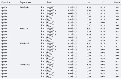
Figure 1a shows the measured gas transfer velocities of CO2plotted against the neutral 10 m wind speed. The
different dependences of thekCO2660onU10Nobserved during the four experiments are immediately
[image:4.612.172.574.124.439.2]appar-ent. While both GasEx data sets show close to cubic wind speed dependence with power lawfit exponents of 2.53 and 2.67 for GasEx-98 and SO GasEx, respectively, an exponent of 1.62 bestfits the HiWinGS data. The Knorr11 data set displays the weakest wind speed dependence with a power law exponent of 1.46. The near-cubic dependences ofkCO2660 withU10Nare in agreement with those reported in Edson et al. (2011)
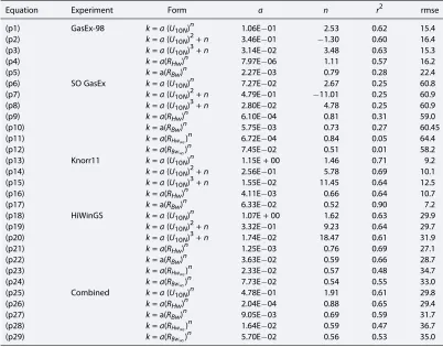
Table 1
Least Squares Fit Results of the Wind Speed and Reynolds Number Dependence of the Gas Transfer Velocity of CO2Referenced
to a Schmidt Number of 660
Equation Experiment Form a n r2 rmse
(p1) GasEx-98 k=a(U10N)n 1.06E01 2.53 0.62 15.4
(p2) k=a(U10N)2+n 3.46E01 1.30 0.60 16.4
(p3) k=a(U10N)3+n 3.14E02 3.48 0.63 15.3
(p4) k=a(RHw)n 7.97E06 1.11 0.57 16.2
(p5) k= a(RBw)n 2.27E03 0.79 0.28 22.4
(p6) SO GasEx k=a(U10N)n 7.27E02 2.67 0.25 60.8
(p7) k=a(U10N)2+n 4.79E01 11.01 0.25 60.9
(p8) k=a(U10N)3+n 2.80E02 4.78 0.25 60.9
(p9) k=a(RHw)n 6.10E04 0.81 0.31 59.0
(p10) k= a(RBw)n 5.75E03 0.73 0.27 60.45
(p11) k=a(RHwws)
n
6.72E04 0.84 0.05 64.4
(p12) k=a(RBwws)
n 7.45E02 0.51 0.01 58.2
(p13) Knorr11 k=a(U10N)n 1.15E + 00 1.46 0.71 9.2
(p14) k=a(U10N)2+n 2.56E01 5.78 0.69 10.1
(p15) k=a(U10N)3+n 1.55E02 11.45 0.64 12.5
(p16) k=a(RHw)n 4.11E03 0.66 0.64 10.7
(p17) k= a(RBw)n 6.33E02 0.52 0.90 7.2
(p18) HiWinGS k=a(U10N)n 1.07E + 00 1.62 0.63 29.9
(p19) k=a(U10N)2+n 3.32E01 9.23 0.64 29.7
(p20) k=a(U10N)3+n 1.74E02 18.47 0.61 31.9
(p21) k=a(RHw)n 1.25E03 0.76 0.69 27.1
(p22) k= a(RBw)n 3.63E02 0.59 0.66 28.7
(p23) k=a(RHwws)
n 2.33E02 0.57 0.48 34.7
(p24) k=a(RBwws)
n
7.73E02 0.54 0.55 33.0
(p25) Combined k=a(U10N)n 4.78E01 1.91 0.61 29.8
(p26) k=a(RHw)n 2.04E04 0.88 0.65 29.4
(p27) k= a(RBw)n 9.05E03 0.69 0.59 31.7
(p28) k=a(RHwws)
n 1.64E02 0.59 0.47 36.7
(p29) k=a(RBwws)
n
and McGillis et al. (2001) for the two GasEx data sets. Quadratic parameterizations reported in Wanninkhof (1992) or Ho et al. (2006) underpredict all but the Knorr11kCO2660.
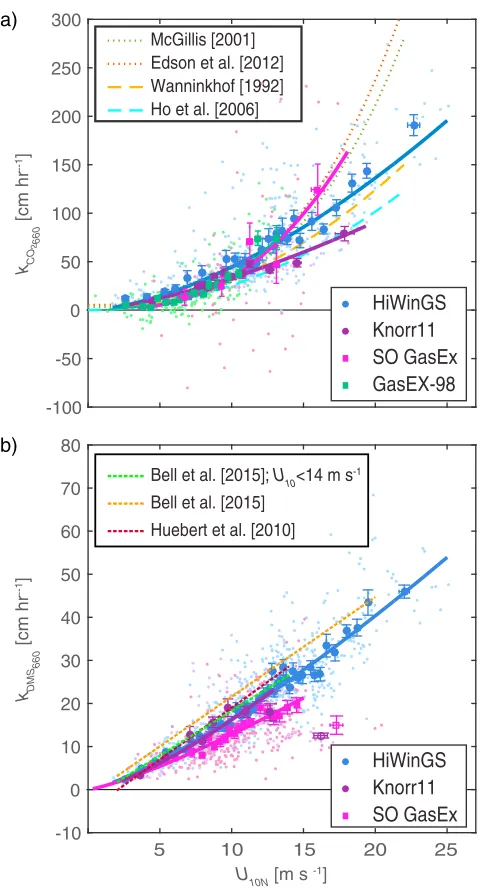
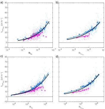
Figure 2a shows that the wave-wind Reynolds number, computed from the total wave spectrum, collapses the observations from all four experiments to a single curve with reduced scatter:
kCO2660¼2:0410
4R
Hw0:88 (5)
withr2= 0.65 and rmse = 29.4 for all data sets combined. Thesefit statistics are slightly better than those obtained from wind-onlyfits (Table 1, equation (p25)). Equation (5) captures 58%, 31%, 63%, and 69% of the observed variability in the GasEx-98 (rmse = 16.4), SO GasEx (rmse = 59.2), Knorr11 (rmse = 13.9), and HiWinGS (rmse = 27.8) measurements, respectively. A wind speed-only power law parameterization based on the combined data set captures 60%, 25%, 70%, and 64% of the observed variability in the GasEx-98 (rmse = 16.3), SO GasEx (rmse = 61.6), Knorr11 (rmse = 16), and HiWinGS (rmse = 30.1) measurements, respectively.
Note that not only were more measurements taken during HiWinGS than during the other experiments, but they were also spread over a wider range of wave and wind conditions. These combinedfits are therefore mostly driven by the HiWinGS data. Nevertheless,fits to individual data sets also demonstrate improved inter–data set agreement with wave-wind Reynolds number compared to wind only. Power law exponents of thesefits, ranging from 0.66 (Knorr11) to 1.11 (GasEx-98), show less spread than those of wind speed power laws. Again, project-specific wave-wind Reynolds numberfits suggest marginal improvement compared to the best individual wind-onlyfits in terms ofr2for HiWinGS and SO GasEx.
The breaking Reynolds number (Figure 2c) also collapses the data sets, with power law exponents ranging from 0.52 (Knorr11) to 0.79 (GasEx-98). However, scatter is increased in comparison to the wind wave Reynolds number for all experiments but GasEx-98. The bestfit obtained from the combination of the data sets is:
kCO2660¼9:0510
3R
Bw0:69 (6)
[image:5.612.172.575.125.388.2]withr2= 0.59 and rmse = 31.7 for all data sets combined. Equation (6) captures 32%, 27%, 89%, and 65% of the observed variability in the GasEx-98 (rmse = 22), SO GasEx (rmse = 60.5), Knorr11 (rmse = 19.2), and
Table 2
Least Squares Fit Results of the Wind Speed and Reynolds Number Dependence of the Gas Transfer Velocity of DMS Referenced to a Schmidt Number of 660
Equation Experiment Form a n r2 Rmse
(p30) SO GasEx k=a(U10N)n 7.31E01 1.25 0.25 5.8
(p31) k=a(U10N)2+n 8.51E02 3.95 0.20 6.4
(p32) k=a(U10N)3+n 5.69E03 6.20 0.13 7.8
(p33) k=a(RHw)n 3.75E02 0.44 0.18 5.9
(p34) k= a(RBw)n 1.91E01 0.35 0.25 5.6
(p35) k=a(RHwws)
n
8.22E01 0.21 0.08 6.1
(p36) k=a(RBwws)
n 3.72E01 0.30 0.22 5.6
(p37) Knorr11 k=a(U10N)n 6.45E01 1.40 0.38 6.0
(p38) k=a(U10N)2+n 1.40E01 2.11 0.34 6.5
(p39) k=a(U10N)3+n 1.11E02 3.78 0.26 7.3
(p40) k=a(RHw)n 7.62E03 0.56 0.20 6.8
(p41) k= a(RBw)n 7.14E02 0.44 0.39 6.3
(p42) HiWinGS k=a(U10N)n 8.23E01 1.30 0.75 5.7
(p43) k=a(U10N)2+n 1.07E01 3.78 0.73 6.2
(p44) k=a(U10N)3+n 5.53E03 6.40 0.65 8.0
(p45) k=a(RHw)n 2.28E02 0.48 0.62 7.0
(p46) k= a(RBw)n 5.73E02 0.47 0.71 6.0
(p47) k=a(RHwws)
n 2.80E01 0.32 0.54 7.0
(p48) k=a(RBwws)
n 3.22E01 0.35 0.63 6.3
(p50) Combined k=a(U10N)n 7.42E01 1.32 0.62 6.5
(p51) k=a(RHw)n 1.95E02 0.49 0.57 6.8
(p52) k= a(RBw)n 5.36E02 0.47 0.63 6.4
(p53) k=a(RHwws)
n 9.95E02 0.39 0.57 7.2
(p54) k=a(RBwws)
n
HiWinGS (rmse = 29.3) measurements, respectively. As for the wave-wind Reynolds number, the close match between the combined and data set-specific fit statistics attest to the inter–data set agreement of these Reynolds number parameterizations.
Utilizing only the wind-sea part of the spectrum to computeHsandωp
does not lead to improved inter–data set agreement based on project-specific fits (Figures 2b and 2d). Compared to full sea state Reynolds numbers, the scatter is increased forRHwws for which the bestfit (Table 1,
equation (p28)) only captures 47% of the variability and there is improve-ment forRBwws which captures 53% (Table 1, equation (p29)) of the
varia-bility of the So GasEx and HiWinGS data combined. Very few good measurements ofkCO2660 were taken during SO GasEx with wind-sea
pre-sent. Therefore, bestfits determined from both data sets are again mainly driven by the HiWinGS data set. Project-specific fits for SO GasEX have
r2≤0.05. Note that for HiWinGS,fits and statistics forRBwwsare very similar
to those forRBw.
3.2. DMS
The parameterkDMS660 measured during SO GasEx was significantly lower
than that measured during HiWinGS for a given wind speed (Figure 1b). The Knorr11 measurements agree with those from HiWinGS for
U10N<10 m s1; however, forU10N> 14 m s1they match the lower
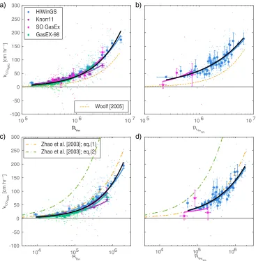
SO GasEx values. The data recorded whenU10Nexceeded 14 m s1during SO GasEx and Knorr11 appear as outliers in Figure 1b as well as in Figures 3a and 3c. They correspond to unfilled bin average data points in thosefigures. The SO GasEx outliers were measured during the return transit leg, and the Knorr11 outliers were measured at the last station under high wind and wave height conditions. No directional wave data are available to separate wind seas from swells for these outliers. They are therefore excluded from Figures 3b and 3d. Sea state, whitecap, and basic environmental conditions do not explain these outliers. They are excluded from results in Table 2. Omitting SO GasEx data taken on the return transit and Knorr11 data forU10N>14 m s1yields better overall
interproject agreement with a power law function of wind speed alone capturing 70% of the variability in the combined data and a rmse of 5.8. The parameter kDMS660 increases close to linearly with wind speed with
power law exponent ranging from 1.28 to 1.4. A power law function of
RHwcaptures 57% of the combined variability with rmse = 6.8:
kDMS660¼1:9510
2R
Hw0:49: (7)
A power law function ofRBwcan account for 63% of the variability in both data sets with rmse of 6.4:
kDMS660 ¼5:3610
2R
Bw0:47: (8)
Considering wind-seas only (Table 2, equations (p53) and (p54)) leads to divergence in the individual bestfits for the two data sets with comparable statistic to equations (7) and (8). As noted above, the high wind SO GasEx and Knorr11 observations were not included in thesefits.
When considering the data sets individually, expressingkDMS660as a function of Reynolds numbers does not
lead to betterfit statistics than wind-onlyfits. Indeed, for SO GasEX a wind speed power law dependence can capture 45% of the variability, while aRBwdependence only captures 25% when ignoring the above
mentioned outliers. For Knorr11, the wind speed andRBwperform comparably well, allowing accounting for 38% and 39% of the observed variability forU10N < 14 m s1. For HiWinGS, the wind speed-only 200 250 -100 -50 0 50 100 150 300 kCO 2660 [cm hr --1 ] a) -10 0 10 20 30 40 50 60 70 80
U10N[m s -1]
25
5 10 15 20
kDMS 660 [cm hr --1 ] b) McGillis [2001] Edson et al. [2012] Wanninkhof [1992] Ho et al. [2006]
Huebert et al. [2010]
HiWinGS
Knorr11
SO GasEx
GasEX-98
HiWinGS
Knorr11
SO GasEx
Bell et al. [2015] [image:6.612.43.284.87.532.2]Bell et al. [2015]; U10<14 m s-1
Figure 1.Measured gas transfer velocity of (a) CO2and (b) DMS, adjusted to
a Schmidt number of 660 and plotted against 10 m neutral wind speed
(U10N). The smaller dots represent individual hourly and 2-hourly estimates,
and the larger symbols are averages of equidensity bins of 15 data points.
The solid lines represent bestfits of power laws of the formk= axn. Examples
of published cubic (k=aU10N3+b) and quadratic (k=aU10N2+b)
para-meterizations derived from CO2data sets are represented by dotted and
dashed lines, respectively. Examples of published linear wind
speed-depen-dent parameterization (k=aU10N+b) derived from DMS measurements are
parameterization performs only slightly better than theRBwone with 75% compared to 71%. Power law
exponents for the fits to the individual data sets are comparably close for wind speed and both Reynolds numbers. It is possible that the potential improvement infit statistics using Reynolds number instead of wind speed is offset by the greater sampling error in determining wave statistics.
4. Discussion
Wind-onlykparameterizations display significant disagreement between different studies (Garbe et al., 2014; Goddijn-Murphy et al., 2012; McGillis et al., 2001; Wanninkhof, 1992). While implementing different wind-only parameterizations for CO2may result in comparable globally averaged gas transfer velocities, the
parameter-ization choice was shown to have significant impact on regionalfluxes (Fangohr & Woolf, 2007; Wrobel & Piskozub, 2016). In light of current efforts to include wave processes in Earth System models (e.g., Li et al., 2016; Qiao et al., 2013), it is time to update the traditional wind-only gas transfer parameterizations to sea state-dependent ones and assess uncertainties linked to the choice of parameterization.
Zhao et al. [2003]; eq.(1) Zhao et al. [2003]; eq.(2)
104 105 106
104 105 106
-100 -50 0 50 100 150 200 250 300
7
RHw ws
10 5 10 6 10 7
RHw
10 5 10 6 10
-100 -50 0 50 100 150 200 250
RBw RBw
ws
c) d)
Woolf [2005]
a) 300 b)
HiWinGS Knorr11 SO GasEx GasEX-98
kCO
2 660
[cm hr
--1
]
kCO 2 660
[cm hr
--1
[image:7.612.191.558.89.463.2]]
Figure 2.Measured gas transfer velocity of CO2adjusted to a Schmidt number of 660 plotted against (a) the wave-wind
Reynolds number based on Hs computed from the total spectrum, (b) the wave-wind Reynolds number based onHs
computed from the wind-sea partition of the wave spectrum, (c) the breaking Reynolds number computed from the total spectrum, and (d) the breaking Reynolds number computed from the wind-sea partition of the wave spectrum. The smaller dots represent individual hourly and 2-hourly estimates; the larger symbols are averages of equidensity bins of 15 data points for Figures 2a and 2c and 5 points for Figures 2b and 2d. The solid green, pink, purple, blue, and black lines represent
Parameterizations that incorporate the dependence of wind and sea state in the form of a wave-wind and breaking Reynolds number provide coherent agreement between the GasEx-98, SO GasEx, Knorr11, and HiWinGS data sets for CO2and the majority of the DMS data. This study therefore strongly suggests that expressingkas a simple function of a wave-related Reynolds number will lead to improved parameterizations for regional and global models relative to wind-only parameterizations. Globalfields of significant wave heights and peak angular velocities are routinely computed by operational wave prediction centers, making wave-wind and breaking Reynolds number-based parameterizations convenient to implement and test on a global scale. The relationships betweenkand other wave statistics such as the wave age, bulk slope, and the mean square steepness were also examined but did not reveal significant trends or yield reduced scatter between projects.
Although the current study is not a comprehensive analysis of all available eddy covariance CO2and DMS gas
transfer data, the data sets analyzed here are representative of the observed variability. They were chosen because they span a wide range of wind speeds with strongly differing dependencies. They are also, to the best of our knowledge, the only available gas transfer data sets with in situ wavefield measurements.
-10 0 10 20 30 40 50 60 70 80
104 105 106
104 105 106
7
RHwws
10 4 10 6 10 7
RHw
10 5 10 6 10
RBw RBw
ws
c)
a) b)
-10 0 10 20 30 40 50 60 70
80 d)
10 5 10 4
kDMS
660
[cm hr
--1
]
kDMS
660
[cm hr
--1
[image:8.612.195.549.88.457.2]]
Figure 3.Measured gas transfer velocity of DMS adjusted to a Schmidt number of 660 plotted against (a) the wave-wind
Reynolds number based on Hs computed from the total spectrum, (b) the wave-wind Reynolds number based onHs
computed from the wind-sea partition of the wave spectrum, (c) the breaking Reynolds number computed from the total spectrum, and (d) the breaking Reynolds number computed from the wind-sea partition of the wave spectrum. The smaller dots represent individual hourly and 2-hourly estimates; the larger symbols are averages of equidensity bins of 15 data
points. The solid pink, purple, blue, and black lines represent bestfits of power laws of the formk= axn, for SO GasEx,
Wave model hindcasts could extend this analysis to other existing CO2and DMS data sets (Bell et al., 2015;
Blomquist et al., 2006; Huebert et al., 2004; Marandino et al., 2007, 2008, 2009; Miller et al., 2009). However, these data sets span a more limited and lower range of wind speeds and may not add much additional infor-mation because discrepancies inkat low wind speeds are small.
CO2and DMS have solubilities of ~1 and ~20, which strongly influence the fraction of total transfer resistance
represented by bubble-mediated and air side mechanisms. The less soluble a gas, the more its air-seaflux depends on the transfer resistance in the aqueous boundary layer and bubble-mediated mechanisms. This explains whykDMSis smaller thankCO2at high wind speeds, where wave breaking leads to generation of
bub-ble clouds and thus the need for different, single parameter models for gases of different solubilities. One could a priori expect DMS to be less sea state-dependent than CO2as its increased solubility means that its transfer velocity depends less on bubble-mediated transfer. Weaker dependence on sea state may account for the increased scatter observed in the relationship between both the wave-wind and breaking Reynolds numbers and kDMS660. Sea state, represented as either the significant wave height or wave age
β¼g=ωpu
¼RBwðgνwÞ=u3), does not reconcile outliers in the SO GasEx and Knorr11 DMS data set.
These suppressed gas transfer velocities at high wind speeds were observed in high wave height conditions; that is, highRHwand more work is needed to understand these observations. Bell et al. (2013) suggest that young, large waves may influence interfacial gas transfer by either causing airflow separation at the wave crest or by modulating the microbreaking of small-scale waves.
Early studies (Toba & Koga, 1986; Zhao & Toba, 2001; Zhao et al., 2003) which relate breaking conditions, whitecapping, and gas transfer velocities to Reynolds numbers focus on wind-sea statistics, ignoring the importance of swell. It is typically assumed that wave breaking is governed by the wind-sea component of the wave spectrum and that properties of the wind-sea partition are most relevant for air-sea processes. This study, however, suggests that consideration of swell is important for gas transfer. Indeed, considering only the wind-sea partition of the wave spectra did not reduce the scatter ink, yielding poorfits that differ substantially between data sets. Arguably, this could be due to the paucity of data collected under wind-sea conditions especially during SO GasEx or the difficulty of separating wind-sea and swell. More data are needed to verify this. However, nonbreaking wave-induced mixing has been shown to significantly contri-bute to upper ocean turbulence through Langmuir circulation (Fan & Griffies, 2014; Li et al., 2016). This sug-gests that mixing that arises from all components of the wave spectra should be considered. Furthermore, if large waves indeed inhibit interfacial gas transfer, the swell component needs to be considered. Reynolds numbers computed from the full spectrum can, however, not account for this effect.
The Reynolds number parameterizations determined in this study differ from previously published parame-terizations (Woolf, 2005; Zhao et al., 2003) using the wind-sea partition or the total spectra. This can partially be attributed to the whitecap data used to tune previous parameterizations. TheWparameterization used by Zhao and Toba (2001) overestimatesWmeasured during both experiments resulting in overestimated gas transfer velocities. The parameterization of Woolf (2005) underestimates the measured transfer velocities of CO2, though it is loosely based on the relation between Wand RHadetermined by Zhao and Toba
(2001). The issue here comes primarily from the relation used between the bubble-mediated transfer and
Wbased on Woolf (1997) but may also be attributed to the expression for nonbreaking transfer used. The coefficients of the 1997 bubble-mediated transfer model are best guess values which were tuned in Woolf (2005) to match a range of observed functions given the assumption that wave fetch is the primary control-ling parameter forW. The model may therefore not be adequate for the open ocean. Note also that we estab-lished that these earlierWdata and the parameterizations differ greatly from recent observations (Brumer et al., 2017) in part due to the different techniques employed and in part due to different wind/wave envir-onments (pure wind versus mixed seas, laboratory or fetch limited versus open ocean waves).
5. Conclusion
observed variability than the traditional wind-only ones. The comparable goodness offits for wind speed and wave-related Reynolds numbers reflects the natural high variability of individualflux estimates which does not vary much for a single set of wind/wave conditions. The important result is that the wave-related Reynolds numbers provide a dramatic improvement in reconcilingkresults from very different wind/wave regimes. Unlike previous studies that relied on the combination of unrelated data sets and approximate rela-tions between Reynolds numbers, whitecap fraction and gas transfer velocities, here we show thefirst Reynolds number parameterizations determined directly from concurrent eddy covariance measurements of gasfluxes and modeled or remotely sensed wavefield statistics.
References
Anguelova, M. D., & Webster, F. (2006). Whitecap coverage from satellite measurements: Afirst step toward modeling the variability of oceanic whitecaps.Journal of Geophysical Research,111, C03017. https://doi.org/10.1029/2005JC003158
Arora, V. K., Boer, G. J., Friedlingstein, P., Eby, M., Jones, C. D., Christian, J. R.,…Wu, T. (2013). Carbon–concentration and carbon–climate feedbacks in CMIP5 Earth System Models.Journal of Climate,26(15), 5289–5314. https://doi.org/10.1175/jcli-d-12-00494.1
Bell, T. G., De Bruyn, W., Marandino, C. A., Miller, S. D., Law, C. S., Smith, M. J., & Saltzman, E. S. (2015). Dimethylsulfide gas transfer coefficients from algal blooms in the Southern Ocean.Atmospheric Chemistry and Physics,15(4), 1783–1794. https://doi.org/10.5194/acp-15-1783-2015 Bell, T. G., De Bruyn, W., Miller, S., Ward, B., Christensen, K., & Saltzman, E. (2013). Air–sea dimethylsulfide (DMS) gas transfer in the North
Atlantic: Evidence for limited interfacial gas exchange at high wind speed.Atmospheric Chemistry and Physics,13(21), 11,073–11,087. Bell, T. G., Landwehr, S., Miller, S. D., de Bruyn, W. J., Callaghan, A., Scanlon, B.,…Saltzman, E. S. (2017). Estimation of bubbled-mediated
air/sea gas exchange from concurrent DMS and CO2transfer velocities at intermediate-high wind speeds.Atmospheric Chemistry and
Physics Discussions,2017, 1–29. https://doi.org/10.5194/acp-2017-85
Blomquist, B. W., Brumer, S. E., Fairall, C. W., Huebert, B. J., Zappa, C. J., Brooks, I. M.,…Pascal, R. W. (2017). Wind speed and sea state dependencies of air-sea gas transfer: Results from the High Wind speed Gas exchange Study (HiWinGS).Journal of Geophysical Research: Oceans,44. https://doi.org/10.002/2017JC013181
Blomquist, B. W., Fairall, C. W., Huebert, B. J., Kieber, D. J., & Westby, G. R. (2006). DMS sea-air transfer velocity: Direct measurements by eddy covariance and parameterization based on the NOAA/COARE gas transfer model.Geophysical Research Letters,33, L07601. https://doi.org/ 10.1029/2006GL025735
Brumer, S. E., Zappa, C. J., Brooks, I. M., Tamura, H., Brown, S. M., Blomquist, B.,…Cifuentes-Lorenzen, A. (2017). Whitecap coverage dependence on wind and wave statistics as observed during SO GasEx and HiWinGS.Journal of Physical Oceanography. https://doi.org/ 10.1175/JPO-D-17-0005.1
Carpenter, L. J., Archer, S. D., & Beale, R. (2012). Ocean-atmosphere trace gas exchange.Chemical Society Reviews,41(19), 6473–6506. https:// doi.org/10.1039/c2cs35121h
Charlson, R. J., Lovelock, J. E., Andreae, M. O., & Warren, S. G. (1987). Oceanic phytoplankton, atmospheric sulphur, cloud albedo and climate.
Nature,326, 655–660.
Christensen, K. H., Röhrs, J., Ward, B., Fer, I., Broström, G., Saetra, Ø., & Breivik, Ø. (2013). Surface wave measurements using a ship-mounted ultrasonic altimeter.Methods in Oceanography,6, 1–15. https://doi.org/10.1016/j.mio.2013.07.002
Cifuentes-Lorenzen, A., Edson, J. B., Zappa, C. J., & Bariteau, L. (2013). A multi-sensor comparison of ocean wave frequency spectra from a research vessel during the Southern Ocean Gas Exchange Experiment.Journal of Atmospheric and Oceanic Technology,30(12), 2907–2925. https://doi.org/10.1175/JTECH-D-12-00181.1
Edson, J. B., Fairall, C. W., Bariteau, L., Zappa, C. J., Cifuentes-Lorenzen, A., McGillis, W. R.,…Helmig, D. (2011). Direct covariance measurement of CO2gas transfer velocity during the 2008 Southern Ocean Gas Exchange Experiment: Wind speed dependency.Journal of Geophysical
Research,116, C00F10. https://doi.org/10.1029/2011JC007022
Fan, Y., & Griffies, S. M. (2014). Impacts of parameterized Langmuir turbulence and nonbreaking wave mixing in global climate simulations.
Journal of Climate,27(12), 4752–4775. https://doi.org/10.1175/jcli-d-13-00583.1
Fangohr, S., & Woolf, D. K. (2007). Application of new parameterizations of gas transfer velocity and their impact on regional and global marine CO2budgets.Journal of Marine Systems,66(1–4), 195–203. https://doi.org/10.1016/j.jmarsys.2006.01.012
Garbe, C. S., Rutgersson, A., Boutin, J., De Leeuw, G., Delille, B., Fairall, C. W.,…Nightingale, P. D. (2014). Transfer across the air-sea interface. In
Ocean-Atmosphere interactions of gases and particles(pp. 55–112). Berlin: Springer.
Goddijn-Murphy, L., Woolf, D. K., & Callaghan, A. H. (2011). Parameterizations and algorithms for oceanic whitecap coverage.Journal of Physical Oceanography,41(4), 742–756.
Goddijn-Murphy, L., Woolf, D. K., & Marandino, C. (2012). Space-based retrievals of air-sea gas transfer velocities using altimeters: Calibration for dimethyl sulfide.Journal of Geophysical Research,117, C08028. https://doi.org/10.1029/2011JC007535
Hanson, J. L., & Phillips, O. M. (2001). Automated analysis of ocean surface directional wave spectra.Journal of Atmospheric and Oceanic Technology,18(2), 277–293. https://doi.org/10.1175/1520-0426(2001)018<0277:AAOOSD>2.0.CO;2
Ho, D. T., Law, C. S., Smith, M. J., Schlosser, P., Harvey, M., & Hill, P. (2006). Measurements of air-sea gas exchange at high wind speeds in the Southern Ocean: Implications for global parameterizations.Geophysical Research Letters,33, L16611. https://doi.org/10.1029/ 2006GL026817
Ho, D. T., Wanninkhof, R., Schlosser, P., Ullman, D. S., Hebert, D., & Sullivan, K. F. (2011). Toward a universal relationship between wind speed and gas exchange: Gas transfer velocities measured with 3He/SF6 during the Southern Ocean Gas Exchange Experiment.Journal of Geophysical Research,116, C00F04. https://doi.org/10.1029/2010JC006854
Huebert, B. J., Blomquist, B. W., Hare, J. E., Fairall, C. W., Johnson, J. E., & Bates, T. S. (2004). Measurement of the sea-air DMSflux and transfer velocity using eddy correlation.Geophysical Research Letters,31, L23113. https://doi.org/10.1029/2004GL021567
Jähne, B., Munnich, K. O., Bosinger, R., Dutzi, A., Huber, W., & Libner, P. (1987). On the parameters influencing air-water gas exchange.Journal of Geophysical Research,92, 1937–1949. https://doi.org/10.1029/JC092iC02p01937
Jähne, B., Wais, T., Memery, L., Caulliez, G., Merlivat, L., Münnich, K. O., & Coantic, M. (1985). He and Rn gas exchange experiments in the large wind-wave facility of IMST.Journal of Geophysical Research,90, 11,989–11,997. https://doi.org/10.1029/JC090iC06p11989
Jeffery, C. D., Robinson, I. S., & Woolf, D. K. (2010). Tuning a physically-based model of the air–sea gas transfer velocity.Ocean Modelling,
31(1–2), 28–35. https://doi.org/10.1016/j.ocemod.2009.09.001
Acknowledgments
Komori, S., Nagaosa, R., & Murakami, Y. (1993). Turbulence structure and mass transfer across a sheared air-water interface in wind-driven turbulence.Journal of Fluid Mechanics,249, 161–183.
Li, Q., Webb, A., Fox-Kemper, B., Craig, A., Danabasoglu, G., Large, W. G., & Vertenstein, M. (2016). Langmuir mixing effects on global climate: WAVEWATCH III in CESM.Ocean Modelling,103, 145–160. https://doi.org/10.1016/j.ocemod.2015.07.020
Liss, P. S., & Merlivat, L. (1986). Air–sea gas exchange rates: Introduction and synthesis. In P. Buat-Ménard (Ed.),The role of air–sea exchange in geochemical cycling(pp. 113–127). Dordrecht, Holland: D. Reidel.
Lund, B., Zappa, C. J., Graber, H. C., & Cifuentes-Lorenzen, A. (2017). Shipboard wave measurements in the Southern Ocean.Journal of Atmospheric and Oceanic Technology,34, 2113–2126. https://doi.org/10.1175/JTECH-D-16-0212.1
Marandino, C. A., De Bruyn, W. J., Miller, S. D., & Saltzman, E. S. (2007). Eddy correlation measurements of the air/seaflux of dimethylsulfide over the North Pacific Ocean.Journal of Geophysical Research,112, D03301. https://doi.org/10.1029/2006JD007293
Marandino, C. A., De Bruyn, W. J., Miller, S. D., & Saltzman, E. S. (2008). DMS air/seaflux and gas transfer coefficients from the North Atlantic summertime coccolithophore bloom.Geophysical Research Letters,35, L23812. https://doi.org/10.1029/2008GL036370
Marandino, C. A., De Bruyn, W. J., Miller, S. D., & Saltzman, E. S. (2009). Open ocean DMS air/seafluxes over the eastern South Pacific Ocean.
Atmospheric Chemistry and Physics,9(2), 345–356. https://doi.org/10.5194/acp-9-345-2009
McGillis, W. R., Edson, J. B., Hare, J. E., & Fairall, C. W. (2001). Direct covariance air-sea CO2fluxes.Journal of Geophysical Research,106, 16,729–16,745. https://doi.org/10.1029/2000JC000506
Miller, S. D., Marandino, C., De Bruyn, W., & Saltzman, E. S. (2009). Air-sea gas exchange of CO2and DMS in the North Atlantic by eddy covariance.Geophysical Research Letters,36, L15816. https://doi.org/10.1029/2009GL038907
Norris, S. J., Brooks, I. M., & Salisbury, D. J. (2013). A wave roughness Reynolds number parameterization of the sea spray sourceflux.
Geophysical Research Letters,40, 4415–4419. https://doi.org/10.1002/grl.50795
Qiao, F., Song, Z., Bao, Y., Song, Y., Shu, Q., Huang, C., & Zhao, W. (2013). Development and evaluation of an Earth System Model with surface gravity waves.Journal of Geophysical Research: Oceans,118, 4514–4524. https://doi.org/10.1002/jgrc.20327
Sweeney, C., Gloor, E. M., Jacobson, A. R., Key, R. M., Mckinley, G., Sarmiento, J. L., & Wanninkhof, R. (2007). Constraining global air-sea gas exchange for CO2with recent bomb
14
C measurements.Global Biogeochemical Cycles,21, GB2015. https://doi.org/10.1029/ 2006GB002784
Toba, Y., & Koga, M. (1986). A parameter describing overall conditions of wave breaking, whitecapping, sea-spray production and wind stress. In E. Monahan, & G. Niocaill (Eds.),Oceanic whitecaps(pp. 37–47). Netherlands: Springer.
Wanninkhof, R. (1992). Relationship between wind speed and gas exchange over the ocean.Journal of Geophysical Research,97, 7373–7382. https://doi.org/10.1029/92JC00188
Wanninkhof, R. (2014). Relationship between wind speed and gas exchange over the ocean revisited.Limnology and Oceanography: Methods,12(6), 351–362. https://doi.org/10.4319/lom.2014.12.351
Wanninkhof, R., & McGillis, W. R. (1999). A cubic relationship between air-sea CO2exchange and wind speed.Geophysical Research Letters,
26(13), 1889–1892.
Wanninkhof, R., Asher, W., & Monahan, E. (1995). The influence of bubbles on air-water gas exchange: Results from gas transfer experiments during WABEX-93, paper presented at Selected Papers from the Third International Symposium on Air–Water Gas Transfer.
Woolf, D. K. (1997). Bubbles and their role in air–sea gas exchange. In P. S. Liss, & R. Duce (Eds.),The sea surface and global change
(pp. 173–206). Cambridge, UK: Cambridge University Press.
Woolf, D. K. (2005). Parameterization of gas transfer velocities and sea-state-dependent wave breaking.Tellus,57B, 87–94.
Wrobel, I., & Piskozub, J. (2016). Effect of gas-transfer velocity parameterization choice on air–sea CO2fluxes in the North Atlantic Ocean and the European Arctic.Ocean Science,12(5), 1091–1103. https://doi.org/10.5194/os-12-1091-2016
Yang, M., Blomquist, B. W., Fairall, C. W., Archer, S. D., & Huebert, B. J. (2011). Air-sea exchange of dimethylsulfide in the Southern Ocean: Measurements from SO GasEx compared to temperate and tropical regions.Journal of Geophysical Research,116, C00F05. https://doi.org/ 10.1029/2010JC006526
Yang, M., Blomquist, B. W., & Nightingale, P. D. (2014). Air-sea exchange of methanol and acetone during HiWinGS: Estimation of air phase, water phase gas transfer velocities.Journal of Geophysical Research: Oceans,119, 7308–7323. https://doi.org/10.1002/2014JC010227 Zhao, D., & Toba, Y. (2001). Dependence of whitecap coverage on wind and wind-wave properties.Journal of Oceanography,57(5), 603–616.
https://doi.org/10.1023/A:1021215904955