This is a repository copy of Valuation of preference-based measures: Can existing
preference data be used to select a smaller sample of health states?.
White Rose Research Online URL for this paper:
http://eprints.whiterose.ac.uk/132955/
Version: Accepted Version
Article:
Kharroubi, S. and Rowen, D.L. orcid.org/0000-0003-3018-5109 (2018) Valuation of
preference-based measures: Can existing preference data be used to select a smaller
sample of health states? European Journal of Health Economics. ISSN 1618-7598
https://doi.org/10.1007/s10198-018-0991-1
[email protected] https://eprints.whiterose.ac.uk/ Reuse
Items deposited in White Rose Research Online are protected by copyright, with all rights reserved unless indicated otherwise. They may be downloaded and/or printed for private study, or other acts as permitted by national copyright laws. The publisher or other rights holders may allow further reproduction and re-use of the full text version. This is indicated by the licence information on the White Rose Research Online record for the item.
Takedown
If you consider content in White Rose Research Online to be in breach of UK law, please notify us by
[1]
Valuation of preference-based measures: Can existing preference data be used to select a smaller sample of health states?
Samer A Kharroubi1 BSc, MSc, PhD Department of Nutrition and Food Sciences
Faculty of Agricultural and Food Sciences American University of Beirut
P.O.BOX: 11-0236 Riad El Solh 1107-2020
Beirut, Lebanon. Tel: 961 1 350 000 Ext 4541
Email: [email protected]
ORCID ID: 0000-0002-2355-2719
Donna Rowen, BSc, MSc, PhD Health Economics and Decision Science
School of Health and Related Research The University of Sheffield Regent Court, 30 Regent Street
Sheffield, S1 4DA Tel: 0114 222 0715 Email: [email protected]
ORCID ID: 0000-0003-3018-5109
Abstract
Background: Different countries have different preferences regarding health, and there are different value sets for
popular preference-based measures across different countries. However, the cost of collecting data to generate country-specific value sets can be prohibitive for countries with smaller population size or low and middle income countries (LMIC). This paper explores whether existing preference weights could be modelled alongside a small own country valuation study to generate representative estimates. This is explored using a case study modelling UK data alongside smaller US samples to generate US estimates. Methods: We analyze EQ-5D valuation data derived from representative samples of the US and UK populations using time trade-off to value 42 health states. A nonparametric Bayesian model was applied to estimate a US value set using the full UK dataset and subsets of the US dataset for 10, 15, 20 and 25 health states. Estimates are compared to a US value set estimated using US values alone using mean predictions and root mean square error. Results: The results suggest that using US data elicited for 20 health states alongside the existing UK data produces similar predicted mean valuations and RMSE as the US value set, while 25 health states produces the exact features. Conclusions: The promising results suggest that existing preference data could be combined with a small valuation study in a new country to generate preference weights, making own country value sets more achievable for LMIC. Further research is encouraged.
Keywords: preference-based health measures; nonparametric Bayesian methods; time trade-off; EQ-5D.
JEL classification: C1; I1.
Acknowledgements: The leading author would like to thank the University Research Bureau (URB) at the
American University of Beirut, Lebanon for funding this study. The authors would particularly like to thank Prof John E Brazier for all his continual support and useful guidance during their time working on this manuscript.
[2]
Valuation of preference-based measures: Can existing preference data be used to select a
smaller sample of health states?
Abstract
Background: Different countries have different preferences regarding health, and there are different value sets for
popular preference-based measures across different countries. However, the cost of collecting data to generate
country-specific value sets can be prohibitive for countries with smaller population size or low and middle income
countries (LMIC). This paper explores whether existing preference weights could be modelled alongside a small
own country valuation study to generate representative estimates. This is explored using a case study modelling UK
data alongside smaller US samples to generate US estimates. Methods: We analyze EQ-5D valuation data derived
from representative samples of the US and UK populations using time trade-off to value 42 health states. A
nonparametric Bayesian model was applied to estimate a US value set using the full UK dataset and subsets of the
US dataset for 10, 15, 20 and 25 health states. Estimates are compared to a US value set estimated using US values
alone using mean predictions and root mean square error. Results: The results suggest that using US data elicited for
20 health states alongside the existing UK data produces similar predicted mean valuations and RMSE as the US
value set, while 25 health states produces the exact features. Conclusions: The promising results suggest that
existing preference data could be combined with a small valuation study in a new country to generate preference
weights, making own country value sets more achievable for LMIC. Further research is encouraged.
[3]
1. Introduction
Health resource allocation is becoming increasingly important in an economic climate of increasing demands on
healthcare systems with constrained budgets. Economic evaluation using cost-utility analysis is becoming a widely
popular technique internationally to inform resource allocation decisions. Cost-utility analysis measures benefits
using Quality Adjusted Life Years (QALYs), a commonly used measure that multiplies a quality adjustment for
health by the duration of that state of health [11]. The quality adjustment weight is generated using utility values
where 1 represents perfect health and 0 represents dead, and is most often generated using an existing
preference-based measure. A preference-preference-based measure consists of a classification system used to describe health (patients
report their own health and this is assigned to a health state using a classification system) and a value set that
generates a utility value for every health state defined by the classification system.
Currently, a number of preference-based measures of health-related quality of life (HRQoL) are available, including
EQ-5D [1], HUI2 and 3 [2, 3], AQoL [4], QWB [5], and SF-6D [6], though there are an increasing number of
condition-specific measures available [7]. The EQ-5D has become a popular measure of HRQoL and there are many
different value sets available for two reasons. First, different countries can have different preferences. Different
countries have different population compositions, different types of work, different cultures, and these can all impact
on the relative values given to different dimensions of health (for example, self-care and anxiety/depression) as well
as where on the 1-0 full health-dead scale each health state lies. The ordering of health states can vary across
countries, as well as the position on the scale in relation to dead. Although Badia et al. [8] reported quite small and
unimportant differences in EQ-5D valuations between UK, US and Spain, it is shown in Johnson et al. [9] that
differences between the US and UK were potentially important. Second, international agencies that review
cost-utility analyses in order to inform resource allocation decisions typically prefer QALYs to be generated using their
own country value set (see Rowen et al. [10] for an overview). This is related to the first reason, as if different
countries have different preferences it is important to take into account the country’s own citizens views when making resource allocation decisions. However, the cost of collecting data to generate country-specific value sets
can be prohibitive for countries with smaller population size or low and middle income countries (LMIC). For
example, if valuation data is collected via face-to-face interview this can be costly and time consuming and the
number of interviews would be in the hundreds. Although valuation data can be collected online, making the data
collection quicker and cheaper, this is not feasible for all countries. For some LMIC the use of an online survey may
be impractical and may not achieve a representative sample of the general population by sociodemographic
characteristics. In addition, understanding of valuation tasks cannot be monitored in an online environment which is
a disadvantage for data collection in countries where valuation tasks have not been undertaken previously. This can
[4]
There is now an increasing number of datasets of preference data, where preferences have been elicited for the same
measure for different countries. In Kharroubi et al [11] a nonparametric Bayesian method is used to model the
differences in EQ-5D valuations between the US and UK as an alternative approach to the parametric
random-effects model of Johnson et al. [9]. Recently, this model has also been applied to the joint Hong Kong and
UK-Japan SF-6D data set ([12], [13]).
Such a model offers a major added advantage as it permits the utilization of the already existing results of one
country to improve those of another, and as such generated utility estimates of the second country will be more
precise than would have been the case if that country’s data was collected and analyzed on its own. Such an analysis (drawing extra information from country 1) may allow a reduction in the sample size in country 2 in order to attain
the same precision as achieved with a complete valuations in that country.
The aim of the paper is to determine whether an accurate value set can be generated for a country using only a small
sample of data collected in that country, through jointly modelling the data with data collected for another country.
This is explored using a case study for US and UK data, where a range of subsets of the health states valued in the
US study are modelled alongside the full UK dataset, and the estimates are compared to the estimates generated
modelling US data alone.
First the US and UK EQ-5D valuation studies as well as the datasets used here are summarised. Second the
Bayesian non-parametric model is described and third the results are presented. Finally, the results are discussed,
including limitations and suggestions of possible directions for future research.
2. EQ-5D data set
The EQ-5D is a descriptive system defined by five health dimensions: mobility, self-care, usual activities,
pain/discomfort and anxiety/depression. Each is assigned to three levels of health-related problems: “no problem” (level 1), “moderate or some problem” (level 2) and “severe problem” (level 3). Different combinations result in 243 possible health states, which are associated with a five-digit descriptor ranging from 11111 for perfect health
and 33333 for the worst state possible. For example, state 13232 translates into no problems in mobility, severe
problems in self-care, moderate problems in usual activities, extreme pain or discomfort and moderate anxiety or
depression [15].
For EQ-5D to be used as a preference-based measure of HRQoL, a single utility value is assigned to each health
state; by convention, utility value of 1 designates full health with all the rest having values less than one. Immediate
death is conventionally assigned the utility zero and is considered as a baseline against the different health states that
[5]
valuation survey undertaken by the Measurement and Valuation of Health (MVH) group at York, using the time
trade off (TTO) technique [16]. A representative sample of 3395 members of the UK general population were
interviewed in their own homes, where they were asked to value 12 health states. The valuation did not include all
243 states defined by the EQ-5D and chose to value a sample of 42 states. Further details on this study are provided
elsewhere [17].
The US valuation study valued an identical set of states using the same UK valuation methods. However a different
approach was used to sample respondents, where a 4-stage clustering sampling strategy was used, that focused on
the Hispanics and non-Hispanic blacks [18]. One further difference was that respondents were interviewed in
English in the UK whereas in the US respondents had the choice of being interviewed in either English or Spanish.
The UK study interviewed a sample of 3395 respondents (response rate: 64%) whereas a sample of 4048 (response
rate 59.4%) respondents were interviewed in the US study. However, respondents were not included due to missing
and/or inconsistent responses. This results in a total of 2997 UK respondents and 3773 US respondents. Both
samples represented their populations in regard to sociodemographic characteristics [17, 18].
Both studies elicited TTO valuations for the 42 EQ-5D health states [17-18]. Briefly, respondents were first asked
whether an impaired health state is better or worse than immediate death. For health states regarded as better than
dead, respondents were asked to choose between living full health for x, years (x≤10) or 10 years spent in the
impaired health state. For states regarded as worse than being dead, respondents were provided the choice of living
in that state for (10-x) years. This is followed by living in perfect health for x years (x<10) or immediate death. The
valuation scores were then transformed using the equation x/10, if states considered as better than death, and in the
UK study -x/10, if states regarded worse than death, in order to bound them on the [-1, 1] scale [19], and in the US
study (-x/(10-x))/-z where z is the worst value produced by -x/10, which is -39 in this case [18].
The UK and US valuations studies also differed in procedures for assigning health states (i.e. 12 states for each
respondent). The US individuals were randomized to receive 1 of 5 groups of pre-defined health states, where 4
groups included 33333 in addition to 2 randomly selected very mild states and 9 states randomly selected from the
remaining 36 EQ-5D states. The 5th group included 33333 and 11 health states selected randomly from the remaining 41 states. In the UK, however, 41 health states (excluding 33333) were stratified into 4 classes according
to severity of problems, where each individual was randomly assigned 2 very mild, 3 mild, 3 moderate, and 3 severe
[6]
3. Modelling
The modelling approach is described in Kharroubi et al. [11], where a nonparametric Bayesian model was used to
model the differences between the US and UK EQ-5D health state valuations, providing an alternative approach to
the conventional parametric model. Using the full US and UK data, Kharroubi et al. [11] found potentially important
differences between the US and UK valuations of EQ-5D. In particular, Kharroubi et al. [11] found that US
individuals give bigger utility values on all of the 42 health states. Because the covariates and respondent random
effects enter the nonparametric Bayesian model multiplicatively, the difference between the two countries was
shown to be minor for good and moderate health states and at its major for the worst health state. In addition, there
seemed to be a substantial interaction between nationality and gender. Kharroubi et al. [11] found that the tendency
to give bigger utilities is stronger for females than for males in the UK, while this is not the case for the US
respondents. Finally, Kharroubi et al. [11] showed that the US respondents are more sensitive to poor health in
mobility and self-care, but less sensitive in the dimensions of usual activities, pain and anxiety. A detailed
description of the analysis is provided in Kharroubi et al. [11].
In this article, we follow on from this work to examine whether the adoption of a range of sample sizes of US health
states (10, 15, 20, 25 states), while borrowing extra evidence from the UK study, generates the same valuations as
analyzing the full US data by itself. The model is estimated using a restricted sample of the US health states (10, 15,
20 and 25) alongside the full UK sample. These estimates are compared to those estimated using all US data
excluding the UK data using different prediction criterion, including predicted versus actual mean health states
valuations, mean predicted error, root mean squared error and an out-of-sample prediction.
For combined analysis, data from the US and UK studies were combined as being derived from one study with
m=6770 respondents. For i = 1, 2, …,
n
j and j = 1,2, …, m, xij is the i thhealth state valued by respondent j and the
dependent variable yij is the TTO valuation given by respondent j for that health state. Finally, let tj be a vector of covariates for respondent j. In particular, tj includes a dummy variable to differentiate respondents’ national identity, but it also includes the respondent’s age and sex.
Kharroubi et al. [11] model the ith valuation by respondent j as
c ij
ij jj
ij
h
u
y
1
exp(
'(
t
)
)
1
(
x
)
, (1)where
h t
(
j)
being a vector of functions of covariates tj and is a vector of unknown coefficients,
j is a random individual effect,
ijis the usual random error,u
c(x
)
is the base utility for the health state vector x and the[7]
is in the UK sample.. It is perhaps easier to understand (1) by writing it in terms of disutilities and
as exp h i.e. simply a multiplicative model with zero
intercept. Then we see that the observed disutility is modelled as the base disutility for the respondent’s
country c, multiplied by the respondent’s effect and then with random error applied. For perfect health,
i.e. and all respondents value it as such apart from the random elicitation errors . For poorer health
states, is larger and respondent covariate and random effects produce larger variations in the elicited values,
thereby accounting for the observed greater variability in respondents’ utilities for poorer health states.
The interpretation of the base utility for country c is that this is the utility function for a respondent from that
country with respondent effect exp h . A respondent with > 1 will exhibit greater disutility
and hence lower utility than the base utility for all states x. The differential is greater for states with low utility than
for those with higher utility (and is zero for perfect health). Conversely a respondent with < 1 will have higher
utilities than the base function for all x, also with increasing differential the lower the base utility of x. This is a key
feature of model (1) that is observed in valuation data, and is one way in which it better represents reality than that
of previous analysis (see Kharroubi et al. [11] for more details).
Kharroubi et al [11] formally assumed normal distributions for the random terms,
j
(
0
,
)
2
N
and
ij N
(
0
,
v
2)
.where
2andv
2are further parameters to be estimated. The distribution of is then log-normal, resulting in askewness that is also typically observed in valuation data.
.
Note that t`s are centred to ensure that they have zeromeans, and hence that the value of for a typical person is 1.
Kharroubi et al. [11] model the relationship between the two base utility functions through
u
0(
x
)
0
0
x
d
(
x
)
, (2))
(
)
(
)
(
)
(
0 11
x
x
d
x
u
0
1
. (3)where
0,
1, 0 and 1 are unknown coefficients andd
(x
)
denotes a shift of the utility function from the[8]
in (3) modifies (2) with additional coefficients 1 in order to reflect dimension-specific differences between the US
and UK [11], but notice they share the same
d
(x
)
function. Hence, we suppose that the utility functions for thetwo nationalities have the same basic shape but can nevertheless differ in important respects.
The term
d
(x
)
is dealt with as an unknown function and so in Bayesian context it will be treated as a randomvariable. Kharroubi et al. [11] assign independent normal distribution to
d
(x
)
as)
(x
d
N
(
0
,
2)
for all x and
,
}
)
(
exp{
))
(
cov(
d
x),
d
(x
'
b
dx
d
x
d' 2 (4)where for d = 1, 2, …, 5,
x
d andx
d' are the levels of dimension d in the health states x andx
, respectively, and bd is a roughness parameter that controls how closely the true utility function is expected to adhere to a linear form in dimension d [14]. The effect of this function is to assert that if x andx
describe very similar, their utilities willbe almost the same, and so the preference function varies smoothly as the health state changes. The key point about
this model is that it allows
d
(x
)
to take any values and hence the utility functions are not constrained in the waythat they are with parametric regression models. It is in this sense that we describe our model as nonparametric, and
we believe that this is another way in which our model is more realistic than that of previous analysis. For more
details on this part of the model see Kharroubi et al. [14].
Subsets of the US sample were selected using systematic random sampling. The sample of 10 US health states was
chosen using systematic random sampling as follows: we first sorted the 42 US health states in increasing order,
then, we selected one health state from the list at random. Every 4th health state from then on has been selected. The systematic random sampling method was adopted in order to make sure that each sampled health state is a fixed
distance apart from those that surround it.
The sampling technique of the 15 US health states is similar selecting each 3rd health state, with a randomly selected health state as starting point. The sampling of the 20 US health states uses the same approach, but with each 2nd health state selected. The sample of 25 US health states was selected as above; that is, with every other health state
being chosen starting from the random selection (baseline).
Given the overall aim of the models is to predict health state valuations, model performance is assessed using
predictive ability, presented using plots of predicted to actual values, calculations of the mean predicted error, root
[9]
4. Results
4.1. 10 US health states
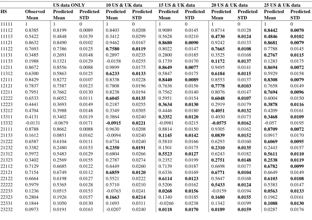
Column 2 of Table 1 displays the actual mean health state utility values of the US data. Columns 3 & 4 show the
predicted mean health state utility values and standard deviation for the US population on its own, while columns 5
& 6 show the predicted population mean health state utility and standard deviation using the 10 health states valued
in the US (in bold font) and UK data (which we shall referred to henceforth as US/UK). As can be seen, the
predicted mean valuations ranged from -0.3082 (33333) to 1 (11111) for the US and from -0.3426 (33333) to 1
(11111) for the (US/UK) population. Figure 1 presents the estimated mean valuations (pink line) for the US
population alone and the observed (blue line) along with the yellow line reflecting the difference between both
values. Figure 2(a) presents the corresponding plots for US/UK population. As depicted from Figure 2(a), the
predicted valuations by employing only 10 health states from the US population, while adopting all the UK data do
not fall in agreement with the observed US valuations. It also shows obvious fluctuations in the predicted US/UK
valuations which in turn justifies the non-steady trend of the difference line. Additionally, the observed RMSE for
the US population by itself is 0.0576, whereas the US/UK achieves a 0.1021, which is almost of double size. Based
on these results, we believe that a sample of 10 US health state is too little and hence more US states are required in
order to get results that are in agreement with those attained with the complete US valuations.
4.2 15 US health states
Columns 7 & 8 of Table 1 show the estimated population mean valuations and standard deviation using the 15
health states valued in the US/UK (in bold font) data. The predicted mean valuations varied from -0.3337 (33333) to
1 (11111) for the (US/UK) population. Figure 2(b) presents the estimated valuations (pink line) for the US/UK
population and the observed mean valuations of the US population (blue line), along with the difference between the
two valuations (yellow line). In comparison with Figure 2(a), the results presented in Figure 2(b) show a little
improvement, although there is still some fluctuations in the predicted US/UK valuations. This is also the case with
RMSE of 0.0883 for the US/UK valuations compared to 0.0576 for the US only. This suggests that 15 US health
state is still a small sample and hence more US states are required in order to get results that are in agreement with
those attained with the complete US valuations.
4.3 20 US health states
Columns 9 & 10 of Table 1 show the estimated population mean valuations and standard deviation using the 20
health states valued in the US/UK (in bold font) data. The predicted mean valuations varied from -0.3105 (33333) to
1 (11111) for the (US/UK) population. Figure 2(c) represents the estimated valuations (pink line) for the US/UK
population and the observed mean valuations of the US population (blue line) as well as the difference between the
[10]
states. In comparison with Figure 1, the predicted valuations by employing only 20 health states from the US
population, while adopting all the UK data are in good agreement with those obtained with the full US sample.
Additionally, the observed RMSE for the US/UK is 0.0665, which is very close to the one obtained using the US
data only (0.0576). Based on these results, we believe a sample of 20 US health states in addition to the whole UK
data might be sufficient to get results that are in quite good agreement with those attained with the complete US
study.
4.3 25 US health states
To be more cautious, we take a step further and look at 25 US health states together with the 42 UK health states.
This is to ensure we get good answers (or even better) as those obtained with the full US study. Columns 11 & 12 in
Table 1 show the predicted population mean valuations and standard deviation using the 25 health states valued in
the US/UK (in bold font) data. The predicted mean valuations varied from -0.3242 (33333) to 1 (11111) for the
(US/UK) population. Figure 2(d) represents the predicted valuations (pink line) for the US/UK population and the
observed mean valuation of the US population (blue line). The yellow line represents their difference. We see from
Figure 2(d) that both valuations are very close for most of the 42 health states. In comparison with Figure 1, the
predicted valuations by employing 25 health states from the US population, while adopting all the UK data are in
perfect agreement. Additionally, the observed RMSE for the US/UK achieves 0.0554, which is very similar to the
one obtained using the US data only (0.0576). This implies that a sample of 25 US health states in addition to the
whole UK data is the ideal scenario needed to adopt in order to obtain results that are in excellent agreement with
those obtained with the full US sample.
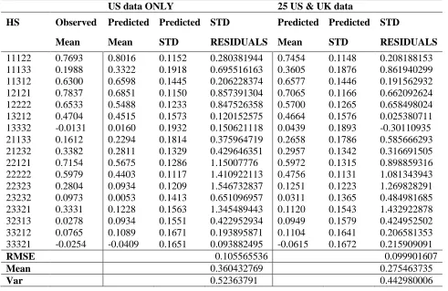
Another comparison of the two approaches is to conduct an out of sample prediction for the remaining health states
that were included in the US valuation survey but not included in the model. Given that 25 US health states were
used for model fitting, we make use of this model to prediction for the remaining 17 health states. Table 2 displays
the true sample means for these 17 missing states, together with the posterior means and standard deviations for
these means in the (US/UK) as well as the US valuations only. It is clear that both estimated value sets are close
most of the health states. However, the predictive performance for the US/UK model is slightly better since the
mean and variance of the standardised prediction errors are 0.275 and 0.443 respectively for US/UK versus 0.3604
and 0.524 for the US only. Additionally, RMSE are slightly better as well, with 0.099 for the US/UK data and
0.1055 for the US only. The better predictions may be observed because the Bayesian model is able to borrow
strength from the UK data (as informative priors), and as such better estimation of the US population utility function
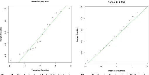
are obtained. For visual checking, Figure 3 shows the standardised prediction errors in two Q-Q normal plots. Panel
(a) plots the errors for estimating the 17 sample means using the US data only, while panel (b) shows the
corresponding errors using the US/UK data. In each case the solid line represents the theoretical N (0,1) distribution.
In theory we would expect the quantiles of the standardised predictive errors to lie roughly on the theoretical line i.e.
[11]
slightly better. This implies that the results obtained are in line with our hypothesis and that there is no need to adopt
more than 25 health states from the US data to obtain the results we are seeking in health states valuations studies.
5. Discussion
Here we have applied a non-parametric Bayesian method to the existing US-UK EQ-5D valuations in an attempt to
determine what size sample in the US EQ-5D health states, while also borrowing extra strength from the UK data, is
needed in order to get answers that are as well as those attained with the full US study. We have shown that, with the
increased number of states considered, we were able to develop a higher accuracy of the results obtained for all
criterion used, including predicted versus actual mean health states valuations, mean predicted error, root mean
square error and an out of sample prediction. Furthermore, we have concluded that a sample of 25 (or even 20) US
health states as well as the whole UK data is the ideal scenario needed to adopt in order to obtain results that are in
excellent agreement with those obtained with the full US sample, based on predictive ability of the models. This is a
promising approach that suggests that existing preference data could be combined with a small valuation study in a
new country to generate preference weights, making own country value sets more achievable for LMIC.
The novelty of the analysis presented here was to use the pooled data when we have a large quantity of observations
on one country and limited observations on another. In the analysis presented here we have shown that drawing
extra information from the first country allows us to reduce the sample size in the second country, and for this to
attain the same precision as we would obtain with a complete data in that country. This kind of analysis could be
extremely important in countries without the same ability to conduct large evaluation studies.
The nonparametric Bayesian model offers a major added advantage: In the existence of lots of observations on one
country and limited on another, it permits the utilization of results of country 1 to improve the results of country 2,
and as such generated utility estimates of the second country may be better than would have been the case if that country’s data was collected and analyzed on its own. This in turn would reduce the need for undertaking large surveys in every country using costly and more often time-consuming face to face interviews with techniques such
as SG and TTO. To our knowledge, this concept hasn’t been investigated properly yet, but clearly it has a lot of
potential value. Further research is underway to assess this.
Limitations of this study include the use of only two datasets as a case study. Value sets can differ across countries
both in terms of the ordering of health states due to differences in relative preferences of the dimensions, and the
location of states on the 1-0 full health-dead scale. Different population compositions, types of work, cultures and
languages can all have an impact, suggesting that this approach may not always produce accurate estimates. The UK
and US populations have different population compositions, yet may be more culturally similar than, for example,
high income and low income countries. This approach may be of most benefit where the samples that are combined
[12]
resources to generate value sets for each individual country generated by combining data collected across different
countries with cultural similarities. The accuracy of estimates may not be at an acceptable level for countries where
there may be larger differences in their health valuations to the larger country whose data is modelled alongside.
Further research is encouraged to examine whether this approach is appropriate using countries which have greater
cultural differences, where relative preferences across different dimensions may differ leading to a different ordering
of mean valuations of health states. This will be useful for informing under what circumstances one country’s values
may be qualified to be modelled alongside the country of interest to generate their value set. In addition, the location
of dead may be a limiting factor, where even if the ordering of states is similar there may be differences in where
these states are located on the 1-0 full health to dead scale. Further research is underway to assess this. In particular,
ongoing research on exploring whether using the UK data might help with the design and analysis of a valuation
study for SF-6D in Hong Kong has preliminary results that are very promising.
One limitation of the approach used to select health states is that the selection was not restricted to the subsample of
states valued by a small sample of people. In the US study there were 5 groups that each valued a different set of
states, and hence here states could have been selected using one group alone, two groups, and then three groups.
However, this should not impact on the results since if new data was being collected with the aim of being analysed
using the Bayesian approach reported here, health state selection could be informed by these analyses.
An additional limitation is that the approach does not explore whether the same results could have been achieved
through keeping the same number of health states and reducing the sample size. However, it is not anticipated that
this would impact on the results, though this can be explored in future research. Furthermore, the Bayesian
non-parametric value sets reported here differ to non-parametric value sets generated for the EQ-5D that are commonly used
to generate QALYs [17, 18], though it is possible that a similar approach could be used to generate parametric
estimates.
Furthermore, as many international agencies recommend the use of country own value sets to generate QALYs, it is unclear whether a value set generated using own country data modelled alongside another country’s dataset would be acceptable. However, this may not be a concern if the estimates are accurate and the ordering of health states and
location on the 1-0 full health-dead scale is similar to those achieved using a large scale valuation study.
In conclusion, the simple idea of pooling the US and UK data proves to be significant in terms of reducing the need
for EQ-5D to be valued separately in each country. The model used in this article could be applied to other
preference-based measures such as SF-6D, 15D and HUI-II, in addition to disease-specific measures where this
[13]
Compliance with Ethical Standards:
Funding: This study was funded by the University Research Bureau (URB) at the American University of Beirut,
Lebanon
Conflict of Interest: The authors declare that they have no conflict of interest.
Ethical approval: This article does not contain any studies with human participants or animals performed by the
[14]
References
1. Brooks R. EuroQol: the current state of play. Health policy. 1996; 37: 53(72).
http://dx.doi.org/10.1016/0168-8510(96)00822-6
2. Torrance GW, Feeny DH, Furlong WJ, et al. Multi-attribute utility function for a comprehensive health
status classification system: Health Utilities Index Mark 2. Medical Care. 1996; 34(7); 702-22.
http://dx.doi.org/10.1097/00005650-199607000-00004
3. Feeny DH, Furlong WJ, Torrance GW, et al. Multi-attribute and single-attribute utility function for the
Health Utility Index Mark 3 system. Medical care. 2002; 40(20): 113(128).
4. Hawthorne G, Richardson G, Atherton_Day N. A comparison of the Assessment of Quality of Life (AQoL)
with four other generic utility instruments. Annals of Medicine. 2001; 33: 358-70.
http://dx.doi.org/10.3109/07853890109002090
5. Kaplan RM, Anderson, JP. A general health policy model: update and application. Health Services
Research 1988; 23: 203–235.
6. Brazier JE, Roberts J, Deverill M. The estimation of a preferencebased measure of health from the SF-36.
Journal of Health Economics. 2002; 21: 271(292). http://dx.doi.org/10.1016/S0167-6296(01)00130-8
7. Rowen DL, Brazier J, Ara R & Azzabi Zouraq I (2017) The Role Of Condition-Specific Preference-Based
Measures In Health Technology Assessment. PharmacoEconomics, 35(Suppl 1), 33-41.
8. Badia X, Roset M, Herdman M. et al. A comparison of United Kingdom and Spanish general population
time trade-off values for EQ-5D health states. Medical Decision Making. 2001; 20: 7-16.
http://dx.doi.org/10.1177/0272989X0102100102
9. Johnson JA, Luo N, Shaw JW, et al. (2005). Valuations of EQ-5D Health States; Are the United States and
United Kingdom Different. Medical Care. 2005; 43: 221-8. http://dx.doi.org/10.1097/0
0005650-200503000-00004
10. Rowen DL, Azzabi Zouraq I, Chevrou-Severac H & van Hout B (2017). International regulations and
recommendations for utility data for health technology assessment. PharmacoEconomics, 35(Suppl 1),
11-19.
11. Kharroubi SA, O’Hagan A, Brazier JE. A comparison of United States and United Kingdom EQ-5D health
state valuations using a non-parametric Bayesian method. Statistics in Medicine. 2010; 29: 1622-34.
http://dx.doi.org/10.1002/sim.3874
12. Kharroubi SA, Brazier J, McGhee S. A comparison of Hong Kong and United Kingdom SF-6D health
states valuations using a non-parametric Bayesian method. Value in Health. 2014; 17(4): 397-405. PMid:
24969000. http://dx.doi.org/10.1016/j.jval.2014.02.011
13. Kharroubi SA. A comparison of Japan and United Kingdom SF-6D health states valuations using a
non-parametric Bayesian method. Applied Health Economics Policy. 2015; 13: 409-20. PMid: 25896874.
[15]
14. Kharroubi SA, O’Hagan A, Brazier JE. Estimating Utilities from individual health state preference data: a
nonparametric Bayesian approach. Applied Statistics. 2005; 54: 879-95.
http://dx.doi.org/10.1111/j.1467-9876.2005.00511.x
15. EuroQol--a new facility for the measurement of health-related quality of life. The EuroQol Group. Health
Policy. 1990; 16(3): p. 199-208.
16. Brazier JE, Ratcliffe J, Tsuchiya A, Solomon J. Measuring and Valuing Health for Economic Evaluation.
Oxford University Press: Oxford, 2007. 19.
17. Dolan P. Modeling valuation for Euroqol health states. Medical Care. 1997; 35:351–363.
18. Shaw JW, Johnson JA, Coons SJ. US valuation of the EQ-5D health states: development and testing of the
D1 valuation model. Medical Care. 2005; 43(3):203-20.
19. Patrick DL, Starks HE, Cain KC, Uhlmann RF, Pearlman RA. Measuring preferences for health states
[16]
Figure 1: Actual (blue line) and predicted (pink line) estimates
[17]
Figure 2: Actual (blue line) and predicted (pink line) estimates and their difference (yellow line) for: (a) 10 US &
UK health states; (b) 15 US & UK health states; (c) 20 US & UK health states; (d) 25 US & UK health states.
(a)
(b)
[18]
Figure 3b: Standardized residuals Q-Q plot for the
US/UK data (25 US health states)
Figure 3a: Standardized residuals Q-Q plot for the
[19]
Table 1: Posterior estimates for various sampled US health states, in addition to the whole US data
US data ONLY 10 US & UK data 15 US & UK data 20 US & UK data 25 US & UK data HS Observed Predicted Predicted Predicted Predicted Predicted Predicted Predicted Predicted Predicted Predicted
Mean Mean STD Mean STD Mean STD Mean STD Mean STD
11111 1 1 0 1 0 1 0 1 0 1 0
11112 0.8385 0.8199 0.0089 0.8403 0.0208 0.9089 0.0145 0.8714 0.0128 0.8442 0.0070
11113 0.5422 0.4848 0.0139 0.3412 0.0299 0.5628 0.0210 0.4730 0.0124 0.4846 0.0102
11121 0.8632 0.8490 0.0102 0.9462 0.0167 0.8680 0.0090 0.9242 0.0133 0.8681 0.0079
11122 0.7693 0.7386 0.0125 0.7580 0.0119 0.8022 0.0147 0.7665 0.0108 0.7788 0.0145
11131 0.3485 0.2691 0.0148 0.2897 0.0235 0.2800 0.0185 0.3525 0.0168 0.2767 0.0115
11133 0.1988 0.1321 0.0129 -0.0158 0.0255 0.1739 0.0170 0.1172 0.0137 0.1283 0.0175
11211 0.8672 0.8556 0.0088 0.9899 0.0175 0.8649 0.0077 0.9495 0.0141 0.8694 0.0072
11312 0.6300 0.5863 0.0125 0.6233 0.0133 0.5847 0.0175 0.6184 0.0115 0.5929 0.0158
12111 0.8429 0.8272 0.0107 0.8338 0.0228 0.8440 0.0089 0.8553 0.0137 0.8308 0.0079
12121 0.7837 0.7587 0.0123 0.7808 0.0196 0.7636 0.0156 0.7778 0.0103 0.7658 0.0149
12211 0.7951 0.7662 0.0130 0.8238 0.0194 0.7562 0.0140 0.8076 0.0147 0.7694 0.0096
12222 0.6533 0.6052 0.0111 0.6045 0.0135 0.5951 0.0154 0.6048 0.0107 0.6004 0.0150
12223 0.4441 0.3693 0.0149 0.2187 0.0255 0.3634 0.0130 0.2919 0.0179 0.3878 0.0116
13212 0.4704 0.3988 0.0148 0.3349 0.0305 0.4446 0.0180 0.4051 0.0132 0.4209 0.0161
13311 0.4131 0.3402 0.0119 0.3864 0.0240 0.3352 0.0120 0.4030 0.0173 0.3468 0.0109
13332 -0.0131 -0.0679 0.0171 -0.0915 0.0221 -0.0981 0.0215 -0.0575 0.0162 -0.057 0.0195
21111 0.8788 0.8662 0.0088 0.9630 0.0208 0.8814 0.0150 0.9305 0.0162 0.8709 0.0072
21133 0.1612 0.0851 0.0162 -0.0094 0.0240 0.1145 0.0142 0.0839 0.0152 0.0917 0.0170
21222 0.6587 0.6104 0.0111 0.6734 0.0240 0.5810 0.0166 0.6293 0.0160 0.6069 0.0095
21232 0.3382 0.2480 0.0153 0.2350 0.0191 0.1501 0.0175 0.2310 0.0135 0.2443 0.0157
21312 0.5972 0.5483 0.0129 0.6804 0.0266 0.5523 0.0127 0.6243 0.0182 0.5611 0.0110
21323 0.3402 0.2569 0.0155 0.2787 0.0274 0.2352 0.0199 0.2751 0.0148 0.2538 0.0119
22112 0.7129 0.6685 0.0122 0.6449 0.0260 0.7139 0.0187 0.6698 0.0177 0.6782 0.0099
22121 0.7154 0.6749 0.0112 0.6859 0.0120 0.6336 0.0169 0.6771 0.0104 0.6649 0.0149
22122 0.6664 0.6198 0.0127 0.5521 0.0222 0.6114 0.0123 0.5647 0.0168 0.6103 0.0108
22222 0.5979 0.5365 0.0128 0.5710 0.0210 0.5206 0.0162 0.5433 0.0124 0.5383 0.0147
22233 0.1236 0.0515 0.0153 -0.0763 0.0241 0.0268 0.0156 -0.0159 0.0194 0.0563 0.0133
22323 0.2804 0.1926 0.0157 0.1663 0.0214 0.1340 0.0185 0.1680 0.0155 0.1962 0.0161
22331 0.1844 0.1050 0.0130 0.1693 0.0311 -0.0266 0.0238 0.1342 0.0199 0.1088 0.0130
[20]
23313 0.1569 0.0814 0.0134 -0.0493 0.0293 0.0536 0.0211 0.0192 0.0200 0.0630 0.0121
23321 0.3331 0.2539 0.0126 0.2549 0.0173 0.1040 0.0203 0.2448 0.0131 0.2449 0.0170
32211 0.2408 0.1783 0.0160 0.2302 0.0254 0.1576 0.0152 0.2438 0.0187 0.1676 0.0120
32223 0.0558 -0.0203 0.0158 -0.1042 0.0229 -0.0284 0.0202 -0.0464 0.0201 -0.0199 0.0130
32232 0.0051 -0.0677 0.0165 -0.048 0.0260 -0.0877 0.0170 -0.0423 0.0167 -0.0457 0.0135
32313 0.0278 -0.0331 0.0152 -0.0612 0.0208 -0.0545 0.0227 -0.0360 0.0171 -0.0312 0.0166
32331 -0.0895 -0.1269 0.0169 -0.020 0.0366 -0.2410 0.0260 -0.0580 0.0210 -0.1259 0.0144
33212 0.0765 0.0097 0.0170 -0.0288 0.0272 0.0190 0.0171 0.0247 0.0154 0.0179 0.0169
33232 -0.1263 -0.1662 0.0169 -0.2106 0.0248 -0.2128 0.0220 -0.1733 0.0199 -0.1733 0.0147
33321 -0.0254 -0.0692 0.0144 0.0154 0.0276 -0.1425 0.0234 -0.0039 0.0198 -0.0752 0.0172
33323 -0.1999 -0.2184 0.0172 -0.2601 0.0276 -0.2311 0.0192 -0.2184 0.0216 -0.2142 0.0153
33333 -0.3460 -0.3082 0.0121 -0.3426 0.0259 -0.3337 0.0186 -0.3105 0.0186 -0.3242 0.0135