An analysis of serial correlation in the errors of linear econometric models

THE ERRORS OF LINEAR ECONOMETRIC MODELS

BY

Athol Kevin Maritz

A thesis submitted to the Australian National University

for the degree of

Master of Economics in Econometrics

Unless otherwise stated, the work in this thesis is the authors own.

TABLE OF CONTENTS

Page

1. HISTORICAL NOTE 1

2. INTRODUCTORY NOTE 2

2a. An Introductory section in which is contained a discussion on the adequacy of the first order

autoregressive model (A R (1))- 3

3. A Section in which we discuss Durbin's test for

serial independence 10

4. In which we apply Durbin's test to Alternative

Models. 21

4a. In which we present a simulation study of the

power of Durbin's test. 27

5. A section in which the admirable findings of

one Michio Hatanaka are presented. 35

5a. In which we look at two other methods used for

estimation of the serially correlated model. 41

PART TWO OF THIS THESIS IN WHICH IS CONSIDERED THE PROBLEM OF SERIAL CORRELATION IN THE CONTEXT OF MULTIPLE EQUATION SYSTEMS

6. A short section in which the model to be studied

is presented. 47

7. A section in which we describe a test for serial independence in the context of simultaneous

equations models. 50

7a. A subsection to note in which are defined

estimators of Type I, II and III. 51

7b. A subsection just preceding the climax in which we present the admirable Guilkey estimator of R,

the matrix of serial correlation parameters. ^5 7c. The climax in which the correct distribution of

the Guilkey estimator is derived and a valid

test deduced. 5 3

APPENDIX 71 72

8. In which we describe an alternative test for serial independence in simultaneous equations

Page 8a. In which we derive the distribution of R. 80 8b. In which the covariance matrix derived in the

previous subsection and written in (8a.6) is

84 evaluated.

8c. Which contains a short discussion comparing

the two tests for serial independence. 87 9. A brief section in which we present Hatanaka's

method for efficient estimation of the dynamic simultaneous equations model with autoregressive

disturbances. 89

10. A section in which we try to reduce the

computational burden to a manageable one. 81 10a. In which we extend the analysis to the

serially correlated model. 188

10b. An extension. H O

APPENDIX 10 I 116

APPENDIX 10 II 119

APPENDIX 10 III 121

11. A concluding section : validity of the model. 123

§1. HISTORICAL NOTE

In the beginning Durbin and Watson gave us the test, Which was then often used when it was not best, To rescue us all from this foolish behaviour, James Durbin again appeared as our saviour.

... for in 1970 he produced a paper containing a test for serial independence valid in the presence of lagged endogenous variables. The basic statistic of the Durbin Watson test is

/\ A " lut-i U k P — 7S. Jk

Eut-1*

where [Ut] is the series of ordinary least squares residuals. In the

/\

absence of lagged endogenous variables p is an asymptotically efficient estimator of p. But not so in their presence. Till Durbin, this had not been fully realized. An incorrect distribution had been assumed and a test with misleading probability of Type I error derived therefrom.

/\

The derivation of the correct distribution for p was merely an application of a more general theory. This thesis consists, in

§2. INTRODUCTORY NOTE

It may validly be asked why we should worry about serial correlation. The following paragraphs give one reason for such a preoccupation.

Consider the familiar linear regression model

Y = X3 + U

Where each element Ut of U has arisen from a distribution with mean 0 and variance 0. If the covariance matrix of U is scalar, it is well known that ordinary least squares is the optimal strategy for estimation of 3. On the other hand, if the covariance matrix is non-scalar,

generalized least squares is the best strategy.

I

The cause of concern is the set of covariances [E (Ut Ut )]. How does one decide whether they are large enough to have to worry about generalized least squares? Because one can extract a scalar constant from the covariance matrix without affecting the value of the generalized least squares estimator, it is clear that it is the size of the

covariances relative to the diagonal term, most easily quantified in terms of the correlation coefficient, that is important. Weight is lent to this conclusion in view of the fact that whereas the covariance is not scale invariant, the correlation coefficient is.

Since T observations is insufficient data to yield meaningful information on the values of T - 1 independent correlation coefficients, we need to specify a relationship between these correlation coefficients involving only a relatively small number of unknown parameters. A reasonable way of doing this is to specify a relationship between the errors [Ut] themselves which will in turn imply a relationship between the correlation coefficients. The most common such relationship is the first order autoregressive model. If [Et] is a white noise process, this model is

§2 a. An introductory section in which is contained a discussion on the adequacy of the first order autoregressive model (AR(1))

Perhaps the major source of serial correlation in the errors of regression models is the omission from explicit consideration of significant variable s that are themselves serially correlated. To see the effect of such an omission consider the case where the true regression equation is

Yt = aYt-1 + ßiXit +32X2t + Et; Et ~ n (O,02)

£

But we omit X2t and try to fit the model

Yt = dYt-1 + 3iXit + Ut

Then Ut = 02X2t + Et. If X2t is serially correlated then so is Ut. In fact if X 2t = 0X2t-l + p t , then the serial correlation induced into the errors of the model we try to fit is

Ut = Et + Ut ( (2a.1)

How well does the simple model Ut = pUt-1 + Et act as a proxy with

respect to (i) detection of the presence or absence of serial correlation and (ii) explanation of the nature of the serial correlation?

Assuming X21 independent of X ^ , its omission, from an estimation viewpoint, is only a cause for concern if it results in the errors being serially correlated to a significant extent. More specifically we can say that the ommission of X2 t will only be a cause for concern if 32

and 0 are of such a size as to cause a significant correlation between Ut and Ut—1 (all other correlations necessarily being smaller if 0 < 1). But under the (mistaken) belief that Ut = put-1 + Et is the true model; p is equal to the correlation between Ut and Ut-1. This model focuses

fortuitous is immaterial. The fact remains that we will use an

estimator of the true correlation coefficient as our estimator of p.

That, under the true model (2a.1), p is not the correlation coefficient

does not harm us. Therefore the model Ut = pUt-1 + Et is likely to

at least do well in detecting the serial correlation induced.

The ability of the AR(1) model Ut = put-1 + Et to act as an

adequate proxy for (2a.1) as far as explanation of the serial correlation

is concerned is another matter. If it is to be adequate than at least

it should predict adequately. We indicate that one could not be confident

that this would be so.

To this end, note that

Ut = Et + I ^ L

=> (I-0L)Ut = (I-0L)Et + B2ht.

But Zt = (1-0L) Et +02t|t, being the sum of two independent moving average

series of order 1 (MA(1)), has a representation as a single MA(1) series

(I-AL)Ct (see for instance the paper by O.D. Anderson [2]). So we have

(I-0L)Ut (I-AL)^t (2a.2)

Ut = (I-AL) (1+0L +02L2 + — ) £t

= (I + (0—A)l + 0(0—A)l2 + — ) ^t

E {utut} = e{ (I + (0-A)L + 0 (0-A) L2 + — ) £t}2 = (I + (0-A)2 + 02 (0-A)2 + — ) a 2

n

= (I + (0-A)2 (1 + 02 + 04 + — )) ay

[I +

0- A)

1- 02

]

y

E(utUt-1} = E [ (1+(0-A)L + 0(0-A)L2 H— )£t) (1+(0-X)L+0(0-X)L2 +-)£t-l)]

= ((0-X) + 0 (0-X)2 + 0 3 (0-A)2 + — )

= ((0-X) + 0 (0-X)2 (I + 02 + — ) a2

= [(0-X) + 0 (0-X)2 ] G2

"ITe*“

n

Hence Corr(Ut,Ut-1) E{UtUt-1} EiutUt}

(0-X) (1-A0) 1 - 20X + Xz

A

Now given Ut, Ut-1, — and an estimate for p, p say, the AR(1)

model would predict Ut+1 via the equation

Ut+1 = put.

Following from the discussion above indicating that p will be an estimate

of the true correlation coefficient, here calculated to be (0-X) (1-A0)

1-20 +

X2-prediction is in effect via the equation

Ut+1 = (an estimate of (0 —X) (1—X0)) Ut /0

” 2 0 - “ F - ( 2 a ' 3 )

From (2a.2) , the proper prediction should be

/\ A A A A A A A A

Ut+1 = (0-A)Ut +X(0-X) Ut-1 + X2 (0-A)Ut-2 + -- (2a.4)

/\ /\

where 0 and X are estimates of 0 and X.

In comparing the two predictions a general statement is not possible;

except, perhaps, to say that it does not seem possible, over the range

of values of 0 and X and {ut-1, Ut-2, — } to show that the predictions

given in (2a.3) and (2a.4) will be the same or even close. One could

not be confident that the AR(1) model will predict well enough. Even if

only because of this shortcoming, one can safely assert that the AR(1)

model will not be an adequate proxy for explanation of the true serial

correlation described in (2a.1).

We have indicated that if X2t = 0 X2t-1 + pt is omitted then the model

This is more likely if (X2t) represents a series of quarterly measure­

ments on the series X2. The serial correlation induced is then

ut = Et + 3i nt 1-0

But according to this model Corr (Ut, Ut-1) = 0 so that the model

Ut = fJUt-1 + Et will tend to accept the hypothesis of serial

independence when correlation does exist. In this case an alter­

native error model Ut = P i+Ut-4 + Et will do a better job of detection.

The two examples given above are very simple. In fact it is likely

that more than one significant variable will be omitted. It is always

possible, though, to derive the serial correlation model induced.

For example, if Xit = OiXit-1 + Ut and X2t = 6 4X21-4 + £t were both

omitted the model induced would be

TTi- - ^2 -rj- £t + Ut + Et I-04L^ s 1-0iL

with an alternative representation as an ARMA(5,5) series. Again either

(I- piL)Ut = Et or (I-p4L 4)Ut = Et is quite likely to detect the

correlation, but neither to explain it.

We have established that the omission of significant variables that

are themselves significantly autocorrelated will probably lead to sig­

nificant autocorrelation in the errors; probably^because it is possible

to obtain a configuration of significant parameters which will yield a small

correlation coefficient .

For example consider again the case of a first order autocorrelated

variable being omitted. From (2a.1), this induces the following

correlation model

Et + $2 I-0L ut

So E(UtUt) = E[(Et + 32(1+ 0L+02L2 + -) Ut)* ]

= a 2 +32 2 (1+02 + 0'*+ - ) a 2

e u

assuming Et and Ut serially uncorrelated and independentof each other.

- 2

Similarly E(UtUt-l) = E [(Et+02 (1+0L+02L2+-)nt)(Et-l+02 (1+0L+02l3~)nt-1)] = 022 (0+03+0 5+ — ) Ü 2

n

It follows that the correlation coefficient is 2 2

corr (Ut, Ut-1 ) = T i-e!) a % n+

0 (1-02 ) + 1 ß2 V 2

2 G 2 2

where r2 = — ^ is the signal to noise ratio. If r2 is very small, ° E

the correlation induced by the omission of X2t will be small irrespective of the magnitude of 0 and 02.

On the other hand, a more serious possibility arises. It is possible that even with a small 02 , the correlation may be large.

Evidently the correlation must be less than or equal to 0. But if r2 is very large, it could offset a small 02 to the extent that the

correlation is very close to 0. If we start with the model Yt = ßiXit + 02 X2t + Et

2

with X21 = 0X2t-l + r|t, and if we let r approach infinity by letting Op approach 0, in the limit we obtain the deterministic model

Yt = BiXit +

02x2t

If X2t is omitted, the error induced is Ut = 02X2t The serial correlation in the error is then

Ut = 0Ut-l + 02nt

The correlation between Ut and Ut-1 is then 0 irrespective of the value of 02 •

The practical implication of this is that when one is working with the type of variable that tends to be serially correlated, as one

typically is in econometrics, one should naturally allow for serial correlation. That is, it should be usual to incorporate serial cor­ relation into the errors of the regression model rather than vice versa.

Consider the other reasonably easily quantifiable source of serial correlation; namely measurement error. This is also particularly likely to occur in an econometric context since economic variables are difficult to measure exactly. Let the true relationship be

Yt = ßxt + Et

But we cannot observe Yt directly. Instead we observe

Y t 1 = Yt + £t (2a.4)

and perform the analysis with this Yt1. Then the actual regression is Y t 1 = ßXt + Et + £t

and the actual regression error is Ut = Et + £t. Now it is eminently possible that we will consistently (under) overestimate Yt. Then serial correlation will be induced into the E,t and hence the Ut.

We propose to suggest a model to explain the time series behaviour Yt and conjecture on a reasonable model to explain the time series behaviour of Yt1. Since (2a.4) in effect defines £t as Yt1 - Yt we can then derive a model for the time series behaviour of £t and hence for the regression errors Ut.

If the time series behaviour of Yt is described by

Yt = 0Yt-l + nt (2a.5)

one might conjecture that the consistent overestimates Yt1 behave similarly. Assume

Yt1 = 0Yt-l1 +At (2a.6)

It follows from (2a.4) that the serial correlation induced into the £t is

£t = Y t 1 - Yt

= OYt-i1 + At - 0Yt-i - nt = ecYt-i1 - Yt) + At - nt

So

Ct = 0^t-i + At - nt

Thus Ut, being the sum of an autoregressive series and an independent series, has a representation as an ARMA series.

§3. A Section in which we discuss

Durbin's test for serial independence

So it is eminently possible for serial correlation to be present in the errors of regression models. A good analyst will therefore concern himself, once confronted by a set of data, with whether serial correlation is actually present. The standard test for serial

independence (in the presence of lagged endogenous variables) is Durbin's test, described in Durbin [8], and briefly reproduced here.

The model is

Yt = a Yt-1 + ßxt + Ut (3.1)

Ut = put-1 + Et ; Et h/ N(0,a2) (3.2)

A

We wish to test Ho : p = 0. If {ut} is the series of residuals resulting from OLS on (3.1), then the estimator of p used is

~ _ Eut-l U t

Z ut-1

Let U be the n.w. element of

(3.3)

j- p lim 1

1> - > oo td 2

w e- 1 » * » r 1

where ^ is the T dimensional vector (X1...XT ) and ^-1 is the T dimensional vector (Yo ...YT-1).

Then under Ho /r p is Ho, T p 2 has a

1 - U

asymptotically N(0,1-U). it follows that under

A

distribution. Substituting an estimator U of

U which is consistent under Ho, this allows us to test Ho.

/N

Durbin's breakthrough was not so much the estimator p used - it had always been used; rather the derivation of its correct distribution. And to do this, Durbin considered the problem rather more generally. A model has two sets of parameters denoted 9^ and J^. The likelihood is

A

L ,^). if oo is some prespecified value of ^ and J3 is the maximizer of

/s

, what is the distribution of that estimator ^ of ^ obtained as /\

In the remainder of this section, we look at the method used by

Durbin to obtain this distribution, remark on the result and finish with

a brief discussion of the power of Durbin's test.

The crucial step in Durbin's derivation is an expansion via the

mean value theorem. Consider such an expansion about the true value

(XT ) of (x , 3) .

/\ /s

0 = 3£(gto,,g ) = 3 £|xt ,Jj*r ) + (£-jgr )32Ity* ,%*) + (ao-ar) 32 £(40*,^*)

(3.4)

0

3£^,jg)

A

= 9A #(gr ) + (£-£x)32£(^**,^**) + ( ^ y )32 £(w**,Z**)

(3.5)

where £ is the log-likelihood and

3|F(Xo) _ 3|F(X) (a)

3x

3x

(b) (i) (^*, j^*) lies between j^to, J3) and (XT , ]3r ) A A

(ii) (^**,7,**) lies between (x , J3) and )

The indeterminateness of (^)*, Z*) and(^f*, ^**) clearly makes it impossible, /\

via this method anyway, to find the distribution o f g e n e r a l l y . The A exceptional case is when ^otT = ao. It can easily be shown that both ^

/\

and 3 are, then, consistent estimators. It follows that asymptotically

%

both (j^3*, ^*) and (üj**, ^**) are equal to the true values ) .

Fortunately, this is all we need to be able to test the hypothesis

^ T = Q\o.

In apparent contradiction to what has been said above, Durbin has

stated that under the hypothesis that otT = a o + - ^ > f°r fixed ^ [si -c(©

has an asymptotic distribution which is N( -A lC'y,A 1 (A-CB 1C I)A x) r \J

where I = [^,^] is the information matrix corresponding to (^).

The reason for the conflict has to do with the peculiarities of

asymptotic theory. It is clear that when D u r b i n [8] reduces the equation

J<J + C'^ ~ B /T (£ - $ ) = 0 (3.6)

he has used the fact that (t)*, Z*) equals (£XX , j^r ) . In effect he A

has used the fact that asymptotically (g^o, J3) = fxx , ) . This is

+ true since OtT

%

y

Y

equals qsymptotically. Durbin has ~7t

assumed that 't is zero asymptotically.

/t

y

On the other hand, when Durbin substitutes ^ for Jtxr - j^o)

V

t

in equation (3.4) to arrive at (3.6), he is using the fact that in

Y

practice T is always finite and so ^ non-zero (though admittedly ✓ T

small). The mere appearance of in (3.6) testifies to this implicit

assumption.

The point is that neither is wrong. But if Durbin was to be Y

consistent in deciding whether % was zero or just small, the apparent

TT"

conflict would not arise.

This sort of thing is done again by Durbin later in his paper [8].

In section 3, when using elements of the information matrix in calculating

the test statistic, some of the quantities used are the calculated

probability limits and others finite sample estimates. For example, the

off diagonal terms of the information matrix are expressed partly in _ pJLim 1 Y-i E and p.lim 1 x'e . ,

terms of t, — % x 'v ^ . These clearly

T— >oo t T — >oo t are zero.

Other elements are expressed in terms o f ^ , ^ ™ ^ ^ - 1 ^ - 1 ' ^ ~ - l ^

. p.lim 1 X ’X. _

and ^ — % % These do not have such an obvious numerical value.

•p— >00 p1

Rather than evaluate them as is done with the term p.lim 1 Y * x E T — >00 rp

instance, the consistent estimates ^ ^-1 etc., are used. The

logical difference in the treatments of the two terms is clear. It

is this that may be the reason for Durbin's h statistic sometimes not

being calculable due to having to take the square root of a negative

number.

Another view of what Durbin has done is that for large T,

X,

ax

approximation to the distribution of ^ .

A

At any rate the point is that the distribution of ^ is exact for Q(T = Q(o and closely approximate for close to^o. Arguably the latter

clause is somewhat trivial. One does not know the distribution of ^

/\

generally. One does not know the distribution of p (defined in

(3.3)) under the alternative hypothesis p = 1. There is a temptation to argue that if we have a thousand observations we need only let

Y = /1000 and then we have the distribution under the alternative ax = ao + 1. But the argument in the previous paragraphs clearly

shows that this cannot be done. It is the size of ^ that is important /t

- T must be large relative to

/N.

If we do not know the distribution of under any alternative

hypothesis how can one, as does Durbin, talk of the power of a test based

-A.

on ^ ? Durbin claims that his test has the same asymptotic power as the likelihood ratio test. How do we reconcile this with the previous discussion?

The likelihood ratio (LR) test is the most powerful test of one simple hypothesis against another. If the alternative is composite and no uniformly most powerful test exists, the likelihood ratio test might be preferred on the grounds that it is locally most powerful. Against one sided alternatives this is tantamount to having out of all tests at ^ocr = £jto the maximum slope of the power function (See Cox & Hinkley [4]).

Since consideration of local power is consideration of alternatives in a very small neighbourhood around the null hypothesis, one can

How attractive this property makes a test is somewhat questionable.

The consequences of rejecting Ho in favour of an alternative in such a

small neighbourhood around <^o are surely not too great. Far more

important is greater power in rejecting consequential alternatives which

may be false.

Consider the Durbin estimator more generally. Using an argument

very similar to Durbin's, equation (3.4) and (3.5) will yield the result

that for scalar a and 3

/ T ( a-ax ) n ( c**c* /t (do -ax ) , 1

a**b* a * * 2

(a** C * * )2

b* (3.7)

a * c

< c „b * > “ d I**

a**c'

( c **k** ) are 1 evaluated at (oo*,Z*) where I*

and (U)**,Z**) respectively.

We compare the estimator with one that is known to be good.

Hence consider the maximum likelihood estimator (M.L.E.) described by

/t ( a

MLE - a x ) ^ N o, (ax - cx 2 ) - 1

where I (

ax cx ÖT

The relative variance is

b X

) is I evaluated at (ax, 3t ) .

(3.8)

v (a)

v(tW

(a**

-*2 _X’

( T - b X >

3 **2

Under the hypothesis ax = ao, this reduces to

X (^ - bx )2

ax 2

(3.9)

or (1 - Fr )

where Ft is the correlation between a and 3.,TT-, under the hypothesis

MLE MLE

car = a o .

The first point to note is that this is less than one, possibly

greatly so. This may appear to contradict the m i n imum variance p r o ­

perty of the MLE. But the MLE is minimum varianced only in the class A

of unbiased estimators: and a is far from unbiased. In fact the most /\

notable characteristic of a is its bias. True that under Ho : ax = a o

the bias is zero (asymptotically). But saying that for some value of a

unbiased-In the latter case the bias is zero for all possible values of a. As one deviates from ax = ao, it becomes unclear as to whether the variance ratio is still Less than one. It depends somewhat on the relative sizes of a** and . One may conjecture, though, that in the case where T is substantial, it is likely that the variance ratio will be less than one.

Let us say that it is not surprising that Durbin's test is locally as powerful as the likelihood ratio test. At OCX = a o , the Durbin

/v /\

estimator a has a smaller variance than a and zero bias. MLE

As one deviates from OtX = ao, even significantly, it is likely that the variance V(a) remains smaller than V(0l ). On the other hand the

MLE A

bias of /t o. certainly increases. In fact the bias becomes very

significant relative to the variance because, as is obvious from (3.7), it is inflated by the ^T factor. However, the impact on power is not immediately obvious.

The question of power is of primary importance to us. Unfortunately, it is not one that I have been able to give a definitive answer to.

However in specific cases one may be able to make an educated guess at whether Durbin's or a test based on the ML estimate will be more powerful.

Actually our aim should be to decide whether the Durbin test is

sufficiently powerful relative to the ML test for it to be worthwhile. The following discussion indicates how one could go about making an educated guess. I emphasize indicate because no definitive answer is obtained. First we obtain a result on power generally. We then use this for a specific model to examine the relative merits of the Durbin and ML test.

Consider the case of testing the null hypothesis Ho : OX = ao against the alternative Hi : ax = a-i. We base the test on an estimater

/s

a of a which n (]i (0) , CT2 (o) ) under Ho and N (y ( i ) , cf2 (i) ) under Hi.

A /\

Y = /

1 (X - y (o))

cr (o)/ai e 2a (o)

d X

/

'ka- y(o)

a(o)

l

/2

t

T

I *2

e 2 d X

Then k = kx} - y (o) is a constant determined only by the significance

0( o)

/\

level independently of a . Power is

1

<x - U(D)2 dx

/s --- e 2 (1)

kx a(i)/27r

00 1 o

1 - X2 d,X

/v --- e 2

ka - y d ) /2tt

a ( i )

“ 1 - i X2 dx

= / --- e 2 p / 2tt

(3.10)

where p = ka - y (1)

a (l)

ka (o) + y (o) - y(l) a (1)

In our case we find that if we use Durbin's estimator a, or since

/\

we are in the asymptotic context, /t a

y (o) = /t a o

y d ) = /t (ao - ( V + / r a t

a 2(o) = 1 (ao - co 2)

ao2 bo

a 2 (1)

1 (a** - c**2 )

I**2 b*

where (w*, Z*) lies between (ao,3) and (a: ,3r ) and (u)**,Z**) lies between

/\

(a, 3), and (a, ,30 and Io = ( . ) is I evaluated at (ao,3 0.

So the P v a l u e c o r r e s p o n d i n g tc/Tot is

P (a) k a** ( ao - Co^/bo)

(a** - c**2 /b*) / 1-r

/ä** /T(l-r**) txo-al)

(3.11)

w h e r e

a* * b * a n d F ** a **b*

On the o t h e r h a n d it is e v i d e n t f r o m (3.8) t h a t the p v a l u e c o r r e s p o n d i n g

A

to /t a %Mr „ is M L E P (cW

where Il

(a, - c r / b l ) (ao - Co"1 /bo)

/t ( a o - a i ) (3.12) ai (1-ri)

( a i ) is I e v a l u a t e d at ( a i , ßr ) a nd Ti

ci b1

ci

ai bi

F r o m (3.10) w e d e d u c e t hat the e s t i m a t o r w i t h the s m a l l e r p v a l u e w ill p r o v i d e the m o r e p o w e r f u l t e s t of Ho : a T = a o a g a i n s t Hi : ai = al .

On c o m p a r i n g (3.10) a nd (3.12) o ne is t e m p t e d to suggest, in v i e w of D u r b i n ' s c o n c l u s i o n on the e q u a l i t y of the p o w e r of t ests b a s e d

Y A

on a a nd ot „ t h a t if we let a , - a o e q u a l --- , t h e n p (a) s h o u l d

M L E , /T

be e q u a l to p ( a £ ) . In fact this w i l l n o t be s t r i c t l y a c c u r a t e in Y v i e w of the p r e v i o u s d i s c u s s i o n s u r r o u n d i n g e q u a t i o n (3.6). If — is

/t large, p(a) and p ( a ^ ) w i l l l i k e l y be s i g n i f i c a n t l y different. If /t

is very small so that a j is very close to ao, then P(a) will be

v e r y c l o s e to R emember, D u r b i n ' s c o n c l u s i o n of e qual p o w e r is o n l y for a l t e r n a t i v e s 'a! c l o s e to the n u l l a o a n d is o nly

A A

a p p r o x i m a t e anyway. T hat be c l°se to P(°0 is clear f rom the fact t h a t in d e f i n i n g (3.10) we use

p(a) k a(o) + y(o) - y(l) a ( i ) 0(1)

a- k x 1 + 0

since if a is c lose to a o , 0(1) ^ cf(o) a n d h(o) a. y(l). S i m i l a r l y for p ( a ). It is a l s o a p p r o x i m a t e l y e q u a l to k. For a i = a o ,

p (a)

Generally, it is difficult to say anything definite about the

/\ /\

relative values of P p ) and P(a ). This is partly because of MLE

the indeterminate nature of (03*, Z*) and (03**, Z**) and partly because the relative p values will undoubtedly vary according to the true

values of unknown parameters. The first terms of p, that is the ratio of standard errors under Ho and , do not depend on whether the

variances themselves are high or low. We would prefer an estimator whose variance under Ho is low relative to its variance under Hj . We

/s

know that V(ot) is low under Ho but it is difficult to say anything definite about the relative sizes of the two variance ratios.

Although the first terms might conceivably be large, one would expect the second terms to be the crucial ones because of the large /t factor.

a* * 1

The comparison is essentially between -— — (1 - T**) a n d — _ . .

1 — I ä 1 (1~1 1 )

The larger of the two leads to greater power since fcxo - 0^) is negative (we are considering a one-sided test with > a o ) . So the

(i_r * *) a**

Durbin test is less powerful if --- — a^ (1 - 1^) is less then one. Granted that T* and T** are different, it would seem that the size of this ratio is going to depend largely on whether a ^ l - T' ) and a**(l - T**) are greater or less than one. We can see this by writing the ratio as

i

-

r**

a**

(i - r**).

a

(i - r )

0.13)

g _ p * *

Although general conclusions on a comparison between ot and a are difficult to make, we can get further with specific examples. Consider the model

MLE

$Yt-l + Ut (3.14)

Ut = aut-l + Et Et % N(0,02 ) (3.15)

It is, in essence, no different to the model we started with in (3.1) and (3.2). Then in Maddala[17] it is shown that

l-OC2 /

P .lint I (Yt-1 - aYt-2):

Furthermore, in Maddala and Rao [18] it is shown that

E(Yt2 ) = g ;

(l-a2) (1-3 T(l-a3)

E (YtYt-l) G2 (a +B )

(l-a2 ) (1-3") (l-a $)

From whence we have that b 1

I^ß2 - so

r

(l-a2 ) (1-32 )

( l - a ß )

7-Consider the quantity a(l-F) which, we have hinted, is likely to

play a crucial role in deciding on the relative merits of the two tests.

In terms of the parameters of the model (3.14) and (3.15), we can express

a(l-T) as

1 , _ ( l ^ x 2 ) ( 1 - 3 2 )

1KX2 [ (l-a 3)2

This is less than one if

(1- a 3)2 - (1-B2) (l-a 2 ) < (1-a2) (l-a 3) 2 (3.16)

iff

2a2 + 32 - l - a 2 32 - 2Dt33 + a 432< o

So the question is whether the function

z = 2 a 2 + B 2 - l - a 232 - 2 a 33 + a 432 (3.17)

is predominantly positive or negative. The easist way of seeing this

is by expressing Z as a quadratic in 3

z - 32 (i - a 2 + a 4) + ß(-2 a 3) - 1 + 2a2

a = -2~> z = ß2 (1 ~ h + + 3 ( - H ) - 1 + h

z = o => 3 =

1 1 I 2 6

4 — ^ I 6_____ 1_6 ZJ>

1 6

=> 3 = 0.95 (since we only admit positive 3). So Z is

negative for all {(a,3) = (^,3), 3 < 0.95.} A similar argument

shows that if a is 1, 3/4 , h and 0 then z is negative for 3 less

than 1, 0.94, 0.98 and 1 respectively. So a ( l - D will almost certainly

j1* *

be less than one. Despite the factor and the fact that a**(l-T**)

is not exactly a(l-T) evaluated at some point, one could be reasonably

On the other hand for 01 = h, the minimum value of Z is about

for ß = 2/1 3- If we let X denote the LHS of the inequality (3.16)

and Y the right, then Z = X - Y and the relevant quantity a(l-F) is X/Y. At worst Z = - F o r a = h, ß = 2/l3, Y = 1 1/i 7. So X -Y =

/2 2Y => /Y = /22 • This gives an idea of how small a(l-T) is and thus a quantitative as well as qualitative indication of the difference in power.

A further indication of the sort of information we can glean despite

A

the inherently non-determinate context is the following. Let ß be the

A A

OLS estimate of ß in (3.14). Let Ut be the residual and a be the OLS estimate of a from Ut = aut-1 + r|t. So a is the Durbin estimate of a. Then it is shown in Malinvaud [19] that and

1*— >00 _L T* pt

Uk-/\ L

p.lim a _ aTßr(ßr + ax)

rj1 -- > 0 O _{1 + ßrax} If ax and ßr are both greater than zero, then in the limit ß > ßr and a < 0^ . Now since w** lies between a and ax it follows that (j o* * • In our example a = /1 -a is an

increasing function of a so that a** <_ a • As fate would have it, this does not allow us to say anything definite about the variance ratio

§ 4 In which we apply Durbin's test to Alternative Models

In the introductory section 2a it was suggested that the first order Markov alternative to serial independence was often not adequate. It was shown that under fairly reasonable assumptions, the actual serial correlation model was likely to be either autoregressive with higher order lags or autoregressive moving average.

Given the specific nature of the behaviour of the omitted variables, it is easy to determine the appropriate error model to use. Unfortunately we can never be sure of exactly what variables were omitted or their

behaviour. We need, therefore to specify a general alternative to serial independence which will do a reasonable job of detecting and explaining the serial correlation, no matter what it actually is. For instance if we use an alternative like Ut = p Ut-k + Et, how

K.

do we decide what k to choose. On the one hand if k is too small we may not detect higher order serial correlation (for example if second order correlation exists, there is no reason why we should detect first order correlation - i.e. no reason why Pi should be significant). On the other hand if we make k too large we may also not detect the true correlation since if first order correlation exists then for example, third will too, but not as significantly.

In view of this, and the moving average nature which seems to characterize the true error models, an obvious improvement over

r

Ut = Ut—1 + Et would be models of the form Ut = • £..p.Ut-i + Et

1=1 i

hoping that a significant correlation between Ut and Ut-i would be

/s

reflected pretty well in a significant p_^.

Therefore, with some justification we follow up the suggestion in Durbin [8] and apply the test set forth in section 3 to these more general Markov alternatives. We wish to test Ho : p i = p2 = . . . =

Yt = E ct Yt-x + E B.Xti + Ut

t . 1 l

T = 1 1=1

(4.1)

Ut = E p. Ut-i + Et , Et ~ N(QCT) i=l 1

(4.2)

Let the number of observations be t = 0, . ., T and let {ut ; t = m

be the residuals resulting from OLS applied to (4.1). Let p =

,T}

(pi, . ., p r ) be the estimators obtained by applying OLS to

^ r /s

Ut = E p Ut-i + Et i=l L

(4.3)

For the last stage there are only T - (m + r) observations over which to

sum (see (4.4)). Although the test is asymptotic so that T is assumed

very large, in practice this is often not so. Therefore there may be

some restriction on the size of- m and r so as to keep the number

T - (m + r) large enough to make the test at least approximately valid.

Then p is the 'Durbin' estimator of

l Let aa = (0t ! ,

• • ' V

3 = (3i,

_{• • V}

P = (Pi, ..,pr )’

(P',

i _ I i

a ,3 ) and 6

and Y = (p , a , 3 ) and 6 = (x ' , 3' ) ' . Let L (Y) be the likelihood

function for the basic random variables {Et} and let the associated

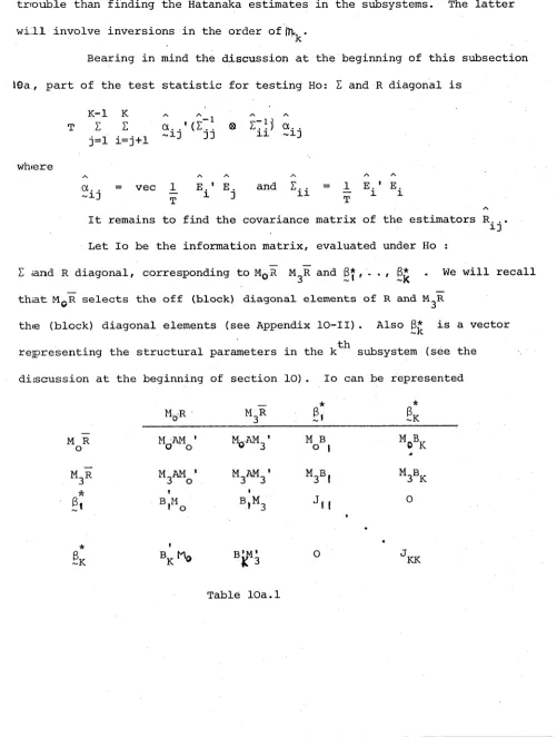
information matrix be

A B C B'D E C'E'F

^ p.lim - 1_ 3 ~ logL (Y) T ->°° T 9 "y9 Y'

where A i s r x r , D i s m x m and F is k x k. Then under Ho the

asymptotic covariance matrix of p is

-1 -1

A a - [b; c] D e'-1"b''

. E'F. C 1

it follows that if Io = I evaluated under Ho, then under Ho

-1 (T - (m+r) )p ' A - [B ; C ] ‘d e - l 1 B '

o o ' o o o o

e'f C '

- o o , L o

Ao P~

i s ’^ 2r. Since Io will in general be a function of the unknown

under Ho the OLS estimates a ,

3

and G 2 = 1 £ Ut2 will be consistent T t=m

/ v

/s /\

estimates of a, 3 and G 2. If Io = Io with the consistent estimates

mentioned above substituted for unknown parameters then under Ho

A. /\

(T - (m+r)) p ' A

/\ - A A

- 1 /s

A A - [B ;c ] D E B

o o o' o o o o

/s /\

e'f C

L o o J o

1-1 ✓s /\

A p O

is asymptotically

if)

r (by the extended Cramer convergence theorem) .

The likelihood function associated with the model described in

equations (4.1) and (4.2) is given by

L(Y)

(/ 2 TT' G )

T-(m+r) exp.

T-(m+r) - 1

2G t=l

(4.4)

a s s u m i n g Et ^ N 0 , G )

=> log L( Y;h2) = k (G2) - 1 2 G :

T-(m+r)

Z

t=l

(Ut - p . U t - 1 - .. p fUt-r)

Noting that Ut = Ut ,

3

) , the log-likelihood is easily differentiated with respect to Y*

In Durbin [8] it is shown that if Y-i is the (T -

f > \ )

x 1 vector

Y . m-i

f 1

for i = 1, . . , m, and Xk is the (T -hl.) x 1 vector

a' ,m,k

V

. V i

for

Z = [Y-l I .... ! Y-mJ XiJ... J Xk] is the (T -»71) x (I'A + K) d a t a m a t r i x , 'N/

then

(i) A

o Ir

(ii) D E o o e'f l o o .

= p . 1 i m . T->°°

1 (T-m) G 2

(iii) C is

o the (r x k) z e r o m a t r i x (iv) B is the (r x m) m a t r i x

1 Yi

^2

0 0

0 0 0 0

Y ,

Y Y

-r-1 r-2 r-3

where Hh is the coefficient of ZJ in the power series expansion of (1 - a,z - ... - a zm ) 1

1 m

A

C = 0 reflects the fact that each p . is asymptotically

o l ,MLE

A

uncorrelated under Ho with each 3, • The form of B means that

k ,MLE o

A /\

p. „ „ „ i s correlated asymptotically under Ho only with a forCT <i.

l , MLE * * 2 j T >MLE _

It is this fact which accounts for Durbin's assertion that with a first order Markov alternative (to serial independence) the introduction of further lags on the endogenous variable does not essentially complicate his test. p .„ is only correlated with a . . On the other hand

l ,MLE i ,MLE

the form of shows that this desirable property does not hold when the error model has higher order lags.

Given the general formulation of Durbin's test and bearing in mind that we have already recommended that r be as large as possible, since attention was originally drawn to the need to consider error models other than Ut = Ut-1 + Et because of the increasing use of quarterly data, the specific examples of Durbin's test to be given will concentrate on the case of r = 4

For r = 4, B is the (4 x m) matrix o

10

1 0 0 0 .. . . 0

[B10 '

Ot 1 1 0 0 .. . . 0

1 2+ 0i2 1 0 .. . . 0

3 + l a p . z + ot 3 a i 2 + c t2 a i 1 .. . . 0

(T - (m + r))P 1 (I4 - Bi q j B ' ) P ^ <p2 (4)

where J is the upper LH ( 4 x 4 ) submatrix of

1

(Z’Z)

(T - (m + 4)cT

- 1

with 0 2

T-m

Ut and

T - m t=l

is with the ax 's replaced by the OLS estimator.

In practice some of the 's and p.'s will be specified a priori

to be zero. In this case the relevant columns and rows respectively

are omitted from B So in general the dimensions of B are as o

follows: number of p ^ 's not specified a priori zero by number of a T 's

not specified a priori zero. For instance, if the alternative is

Ut = p .U t — 1 + p.Ut-4 + Et, the second and third rows of B are

l 4 o

omitted to yield

B 0 0 0 0 0 . . . 0

Ot j 3 + 2 Ot i0t 2 + Ot 3 0tj2+ 0t2 Ot i 1 Q . . . 0

J is as before - the upper LH (4 x 4) submatrix

If, as well, a 3 is specified zero and Yt-3 is not included in the

regression, then we omit the third column of B^ to obtain

a i3 +2ctia2 a j2+ a2 1

0 0

0

(zero has been substituted for ot 3 in the general expression for B ).

In this latter case Z = [Y-l, Y-2, Y-4 ...

and J is the upper LH (3 x 3) submatrix of

Y-m; X! ... Xk ]

(Z'Z) (T - (m + 4)Cb

-1

T-m

with O’" 1 Ut as before.

T -m t=l

A further case sure to be used in practice when confronted with

quarterly data is the alternative Ut = p^Ut-4 + Et. For the regression

B = [oil3 + 2aioi2 + a 3, a !2 + a 2 , a i 1,0 ___ o 1

o

The t est s t a t i s t i c is then

A

(T - (m + 4) P 4 2 ^

p

2 (1) (4.5)

A

1 - U

w h e r e if J is the u pper LH ( 4 x 4 ) s u b m a t r i x of JL________ (Z'Z) andA (T - (m +

4'fj

Q 2 is the O LS e s t i m a t e of the i e l e m e n t of Bq , then

4 4

U =

Z

Z

X. J. .X.

. . ... i id 3

i=l 3=1

F i n a l l y w h e n t e s t i n g for se r i a l i n d e p e n d e n c e of the e r r o r s of the k

r e g r e s s i o n m o d e l Yt = a Y t - 1 +

Z

ß X + Ut a g a i n s t the a l t e r n a t i v e k=l k tk

Ut = put-4 + Et, the a p p r o p r i a t e test s t a t i s t i c is (T - 5)

p z

„

1 - (T-5)V(tt)

OL

"u p 2 (1)

w h e r e V (a) is the v a r i a n c e of the OLS e s t i m a t e of a w i t h A

3 s u b s t i t u t e d for a a nd ß.

~ (JLo ~

OLS a nd

It is i n t e r e s t i n g to c o m p a r e this to the t est d e r i v e d by D u r b i n for the a l t e r n a t i v e Ut = put-1 + Et. F or this case the a p p r o p r i a t e test s t a t i s t i c w a s

(T - 2) p2 ^ 1 - (T-2) V (a )a 0

^ P 2

(1)

G e n e r a l l y for the a l t e r n a t i v e Ut s t a t i s t i c w i l l be

A

(T - (r + 1) p 2

7s 7T Al(r-l)

p U t - r + E t , the a p p r o p r i a t e t e s t

§4a In which we present a simulation study of the power of Durbin's test.

In section 3 we attempted to investigate the power of Durbin's test by analytical means. Another possibility is by an empirical study. In this section we report the results of such a study using artificially generated data.

The model looked at is Yt = CXYt-1 +

ßxt

+ Ut Xt

Ut

A x t - i + n t f v ( n t ) =

put-4 + Et

, V

(Et)

= a

2

(4a.1) (4a.2) (4a.3) Specifically, we have investigated the performance of Durbin's test of Ho : p = 0. The test statistic is as in (4.5) with m = 1.

Following the reasoning of Maddala and Rao [17], we will assume that

2

O 2 2

it is through T = U that 0 and O may have an effect on the

a2 n e

e

probability of making Type I and Type II errors. Also we assume that 3 will have no effect on the probability of making these errors. For the duration of the study we let ß = 2.

The parameters, the effects of which we will investigate, are then

r, A, ot,

p and the number of observations T. We let T take the high value 25 and the low value 5. We let

A,

a and p take the values 0.3, 0.6 and 0.9 in turn. We let T take the high value 100

representing 25 years of quarterly data and the low value 20. We have not looked at what happens when there are further lags on Yt in

(4a.1) and Xt in (4a.2). It is quite possible that if the auto­ regressive model (4a.2) were fourth order the conclusions regarding the effects of

A

would be different.

Firstly consider the probability of making a Type I error. We let p= 0 and look at the proportion of times the hypothesis Ho :

3.84 in 100 r e p l i c a t i o n s . If X d i s t r i b u t i o n , the n P r (X < 3.84)

2 is a r a n d o m v a r i a b l e w i t h a (1)

95 100

T =

A

= 0 . 3

A

= O.i

a = 0 . 3 97 96

r = 5 a = 0 . 6 92 93

0i = 0 . 9 9 5 96

a = 0 . 3 93 9 6 T= 25 a = 0 . 6 94 93

CL = 0 . 9 94 9 4

Ta ble

20 T = 100

A

= 0 . 9 A = 0 . 3

A = 0.6

ii o

94 96 96 96

95 95 95 95

95 96 96 95

95 95 97 95

93 96 96 93

95 96 95 94

4a. 1

Fo r a g iven

A, a, T

a nd T, if the t est s t a t i s t i c a c t u a l l y h as a

’p 2

(1) d i s t r i b u t i o n on e w o u l d e x p e c t an e n t r y of 95 in Table 4 a . 1. S t r i c t l y s p e a k i n g this w o u l d n o t be s u f f i c i e n t to p rove that the test s t a t i s t i c a c t u a l l y has a

ip

(1) d i s t r i b u t i o n but we do not p u r s u e this point.

The firs t p o i n t to no te is t hat for T = 100 the res u l t s are as expected. For T = 20 it w o u l d n ot have b e e n s u r p r i s i n g to find the e n t r i e s

s i g n i f i c a n t l y d i f f e r e n t fro m 95 b e c a u s e for T = 20 one c ould h a r d l y expect the tes t s t a t i s t i c to be

'{

j (1). Yet, we are p l e a s a n t l y s u r p r i s e d to find the e n t r i e s no t m a r k e d l y d i f f e r e n t from 95. F r o m the p o i n t of v i e w of the 0.05 p e r c e n t a g e point, e v e n for T = 20, the test s t a t i s t i c se e m s to be n e a r l y

'j)

(1).

S i n c e the c o r r e c t s i g n i f i c a n c e level seems a p p r o x i m a t e l y to have b een a t t a i n e d for b o t h T = 20 an d T = 100, we can i n t e r p r e t 1

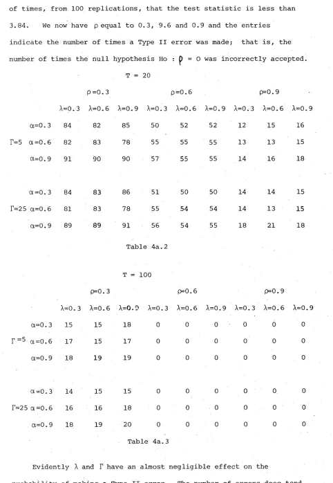
In the following two tables the entries again represent the number

of times, from 100 replications, that the test statistic is less than

3.84. We now have p equal to 0.3, 9.6 and 0.9 and the entries

indicate the number of times a Type II error was made; that is, the

number of times the null hypothesis Ho : p = 0 was incorrectly accepted.

T = 20

f}=0. 3 P=0.6 p=0.9

A=0.3 A=0.6 A=0.9 A= 0 .3 A=0.6 A=0.9 A=0.3 A =0.6 A=0.9

ot=0.3 84 82 85 50 52 52 12 15 16

F=5 Ot =0.6 82 83 78 55 55 55 13 13 15

a=o.9 91 90 90 57 55 55 14 16 18

a=o. 3 84 83 86 51 50 50 14 14 15

r=25 a=0.6 81 83 78 55 54 54 14 13 15

p II o vo 89 89 91 56 54 55 18 21 18

Table 4a.2

T =: 100

p=0. 3 p=0.6 p=0.9

A=0. 3 A=0.6 A=0.9 A=0.3 A=0.6 A= 0 .9 A =0.3 A= 0 .6 A=0.9

a=0. 3 15 15 18 0 0 0 0 0 0

r = 5 a =0. 6 17 15 17 0 0 0 0 0 0

p II o VO 18 19 19 0 0 0 0 0 0

a = 0 . 3 14 15 15 0 0 0 0 0 0

T=25 a =0.6 16 16 18 0 0 0 0 0 0

P ii o VO 18 19 20 0 0 0 0 0 0

Table 4a.3

Evidently

A

and

T

have an almost negligible effect on the

[image:34.556.43.525.62.760.2]

to increase with increasing a though this effect is not terribly pronounced. The variables with by far the greatest effect on power

are, not surprisingly, p and T. In fact the most striking aspect of the two tables 4a.2 and 4a.3 are on the one hand the atrocious per­

formance of the test when T = 20 and p = 0.3 and on the other its

seeming infallibility when T = 100 and p = 0.6. The extreme difference in performance between the cases when T = 20 and T = 100 is a little surprising in view of the fact that for T = 20 the correct significance level was very nearly obtained. Perhaps the latter aspect is the more surprising.

In view of the fact that T = 20 is very low and T = 100 is very high and that the performance of the test differs markedly between these two values, it would be of interest to investigate values of T in between these two extreme values. Hence contemplate Table 4a.4. For it we have kept A = 0.6, ot = 0.6 and F = 15. Again the entries are the number of times, from 100 replications, that the test statistic is less than 3.84.

T = 20

p = 0.0 93

p = 0.3 83

p = 0 . 6 55

p = 0.9 13

Table 4a.4

= 40 T = 60 t = :

94 97 95

59 45 15

11 1 0

0 0 0

We have assumed that the values for T = 15 are about the average of the values for F = 5 and T = 25. This is not a strong assumption because the values for

T

= 5 and

T

= 25 (with a = A = 0.6) are as close as can be anyway.

The most pleasing aspect of Tables 4a.2, 4a.3 and 4a.4 is the almost infallible performance of the test for T = 60 and P =0.6. One further small table is of interest. Let a =

X

= 0.6,

T

= 15 and T = 100. The entries in the following table are the number of times the test statistic, from 100 replications, is less than 3.84.

p = 0.3 15

p = 0.4 3

p = 0.5 0

p = 0.6 0

Table 4a.5

The most disturbing aspect of the results presented in Table 4a.4 is that for T less than about 50 and p less than about 0.4, we can expect to incorrectly accept the null hypothesis more than half the time.

Because we know the distribution of the ML estimator of P under any hypothesis, we can, for large samples, give the power of a test based on the ML estimator by analytical means. We know that if the parameters are divided into two sets a and 3 with corresponding information matrix

, then the asymptotic distribution of the ML estimator ot

of Ot is given by

/

v

,

— —

i

/t (a - a) ^ N(0,

{

a

-

c 'b ) (4a.4)

MLE

(compare with equation (3.8))

We intend only to look at the model

Yt = aYt-1 + Ut (4a. 5)

Ut = pUt-4 + Et , V(Et) =

o2

(4a.6)

We conjecture that the exclusion of an exogenous variable will not significantly affect power. For the simulation study of Durbin's test we implicitly assumed that ß (defined in 4a.1) has little effect

A C C 'b

A

a nd

F

h ad no s i g n i f i c a n t e f f e c t on the p o w e r of D u r b i n ' s test. Let the i n f o r m a t i o n m a t r i x c o r r e s p o n d i n g to / p\ be /a c\

l o t / l c b /

T hen a = p . l i m 1 £ (Yt-4 - a Y t - 5 ) ^ T ->°° T 0 ?

w h i c h e q u a l s (using r e s u l t s in W a l l i s [27])

(1 + a 1 (1 + a 4p) - 2g. g (1 -to2p )

( 1 - a 2 ) ( l - p 2 ) ( 1 - g 4 p) ( l " - g 2 ) ( l - p 2 ) ( l - g 4p )

w h i c h in tu rn e q u a l s 1

l - p 2 (4a.7)

A l s o b = p . l i m 1 £ (Yt-1 - p Y t - 5 ) 2 T ->°° T O 2

A g a i n u s i n g r e s u l t s in W a l l i s [27] w e find that thi s equ als

(1 + p2 ) (i -tg4p ) - 2 p. (a 44p ) (1 + a 4p )

(1-a2 ) (1- p2 ) (1-a4 p) l+ a 4p (1-a2 ) (l-p 2 ) (1-a 4p )

w h i c h eq u a l s

1 -a" (4a. 8)

L a s t l y c p . l i m 1 T- >°° TO ‘

£ (Yt-4 - a Y t - 5 ) ( Y t - l - pYt-5) Thi s equ a l s

a (a2 4p ) pa (1 -na2p ) a ( a f+p )

(1-a2 ) (l-p*) (1-a4 p) (1-a2 ) (l-p2) (1k x4p) (1-a2 ) (l-p2 ) (l-<x4 p )

+ ap(l +a p)

(1-a2 ) (l-pz ) (l-g 4 p)

w h i c h eq u a l s

1 - g p (4a.9)

A g a i n let N( y (o),G2 (o)) and N ( y (1) ,02 (1)) be the d i s t r i b u t i o n s of /r a un der Ho a nd Hj. A s s u m i n g a = 0 . 6 and T = 100, c o n s i d e r

ML E

tes t i n g Ho : p = O a g a i n s t Hi : p = 0.3. T h e n u s i n g e q u a t i o n s 4 a . 4, 4 a . 7, 4 a . 8 a nd 4 a . 9, w e h a v e that

P(o) = 0

y (i) = /t

p

= 1 0 x 0 . 3 = 1

4

a

2(o)

a

2

(i)

/ 5

kO (o) +0 (o) - yi (1) = k x 1 + 0 - 3

0(1) 0.9

For a test with significance level 0.05, k = 1.64. So P =

-1.51. The power of the test is then (see equation (3.10)).

oo -i^x2

f

-- 7 dx = 0.93

-1.51 /2r

The first entry of Table 4a.5 indicates that the power of Durbin's test for p = 0 when p actually equals 0.3 is 0.85. Although the tests have the same local power, it appears that p = 0.3 is not in the locality of p = O. On the other hand the powers of the two tests is pleasingly close.

The results on the power of Durbin's test for T = 50 andp = 0.4 are more disturbing than one at first realizes. We would always like the probability of making a Type II error to be small. But usually this is not our primary concern in hypothesis testing. Within the Neymann-Pearson theory ones preoccupation is with Type I error. It is this that we can control and keep rare. Implicit in the whole theory is the assumption that to make a Type I error (rejecting the null hypothesis when it is true) is more serious than to make a Type II error (accepting the null hypothesis when it is false). Yet this is clearly not the case when we are testing for serial independence. Accepting the fact that we have an adequate theory for analysing the serially correlated model, it is preferable to incorrectly reject the null hypothesis rather than to incorrectly accept it. This is because if the null hypothesis is incorrectly rejected, this is likely to show through in subsequent analysis. On the other hand if the null hypothesis is incorrectly accepted subsequent analysis is much less likely, at

It follows that in cases for which the Durbin test does not have good power its usefulness is highly questionable. This statement can be