fog/cloud computing systems
.
White Rose Research Online URL for this paper:
http://eprints.whiterose.ac.uk/136368/
Version: Accepted Version
Article:
Du, J., Zhao, L., Chu, X. orcid.org/0000-0003-1863-6149 et al. (3 more authors) (2018)
Enabling low-latency applications in LTE-A based mixed fog/cloud computing systems.
IEEE Transactions on Vehicular Technology. ISSN 0018-9545
https://doi.org/10.1109/TVT.2018.2882991
© 2018 IEEE. Personal use of this material is permitted. Permission from IEEE must be
obtained for all other users, including reprinting/ republishing this material for advertising or
promotional purposes, creating new collective works for resale or redistribution to servers
or lists, or reuse of any copyrighted components of this work in other works. Reproduced
in accordance with the publisher's self-archiving policy.
[email protected] https://eprints.whiterose.ac.uk/ Reuse
Items deposited in White Rose Research Online are protected by copyright, with all rights reserved unless indicated otherwise. They may be downloaded and/or printed for private study, or other acts as permitted by national copyright laws. The publisher or other rights holders may allow further reproduction and re-use of the full text version. This is indicated by the licence information on the White Rose Research Online record for the item.
Takedown
If you consider content in White Rose Research Online to be in breach of UK law, please notify us by
Enabling Low-Latency Applications in LTE-A
Based Mixed Fog/Cloud Computing Systems
Jianbo Du, Liqiang Zhao
Member, IEEE
, Xiaoli Chu
Senior Member, IEEE
, F. Richard Yu
Fellow, IEEE
, Jie
Feng, and Chih-Lin I
Senior Member, IEEE
Abstract—In order to enable low-latency computation-intensive applications for mobile user equipments (UEs), com-putation offloading becomes critical necessary. We tackle the computation offloading problem in a mixed fog and cloud computing system, which is composed of an LTE-A small-cell based fog node, a powerful cloud center, and a group of UEs. The optimization problem is formulated into a mixed-integer non-linear programming (MINLP) problem, and through a joint optimization of offloading decision making, computation resource allocation, resource block (RB) assignment, and power distribution, the maximum delay among all the UEs is minimized. Due to its mixed combinatory, we propose a low-complexity iterative suboptimal algorithm called FAJORA to solve it. In FAJORA, first, offloading decisions are obtained via binary tailored fireworks algorithm (FA); then computation resources are allocated by bisection algorithm. Limited by the uplink LTE-A constraints, we allocate feasible RB patterns instead of RBs, and then distribute power among the RBs of each pattern, where Lagrangian dual decomposition is adopted. Since one UE may be allocated with multiple feasible patterns, we propose a novel heuristic algorithm for each UE to extract the optimal pattern from its allocated patterns. Simulation results verify the convergence of the proposed iterative algorithms, and exhibit significant performance gains could be obtained compared with other algorithms.
Index Terms—Computation offloading, fireworks algorithm, fog computing, LTE-A, resource allocation.
I. INTRODUCTION
With the proliferation of smart user equipments (UEs) and the popularity of low-latency applications [1], the current mobile networks have been pushed to their limits. Mobile cloud computing (MCC) [2] has appeared as a potential way to cope with the above challenges by offloading computations to powerful cloud servers. More recently, fog computing [3] (or mobile edge computing (MEC) [4]) has been put forwarded as an effective complement to MCC and has been deemed as an important paradigm and scenario in 5G [5].
*This work was supported in part by National Natural Science Founda-tion of China (61771358), NaFounda-tional Natural Science FoundaFounda-tion of Shaanx-i ProvShaanx-ince (2018JM6052), Intergovernmental InternatShaanx-ional CooperatShaanx-ion on Science and Technology Innovation (2016YFE0123200), the Fundamental Research Funds for the Central Universities, and the 111 Project (B08038).
J. Du, L. Zhao, J. Feng are with State Key Laboratory of ISN, Xidian University, No.2 Taibainan-lu, Xi’an, 710071, Shaanxi, China. (Email: [email protected]; [email protected]; [email protected]).
X. Chu is with Department of Electronic and Electrical Engineering, The University of Sheffield, Mappin Street, Sheffield, S1 3JD, UK. (Email: [email protected]).
F. R. Yu is with the Dept. of Systems and Computer Eng., Carleton University, Ottawa, ON, Canada (e-mail: [email protected]).
C.-L. I is with the Green Communication Research Center, China Mobile Research Institute, Beijing 100053, China. (e-mail: [email protected]).
By setting up a virtualized platform between UEs and cloud centers, fog computing can provide computation, storage, and networking services [6], [7] to nearby UEs, and thus to further enhance network performance in energy conservation or delay reduction [5].
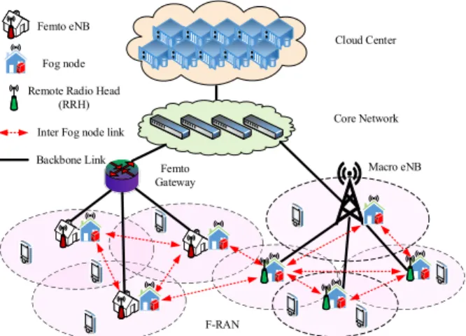
Fig.1 shows the typical architecture of a mixed fog/cloud computing system. Utilizing the computation resources of the fog nodes, such as WiFi access points (APs), base stations (BSs), or remote radio heads (RRHs), fog nodes can offer computation services at the edge of the network [3], [4]. Fog nodes can communicate directly with each other, and all the fog nodes are connected to the powerful cloud server through high-speed wired links [3], [4]. The cooperation between the cloud server and the fog nodes can provide users with more efficient and appropriate computation offloading services. However, this new architecture brings many new problems, e.g., how does the fog cooperate with the cloud, i.e., where should computation be offloaded to, and how the resource be allocated, etc., so as to bring the advantages of the new architecture into full play.
In this paper, in order to enable low-latency compute-intensive user applications with fairness among UEs guaran-teed, we propose to minimize the maximum delay consump-tion among all UEs in an LTE-A based mixed fog/cloud com-puting system by jointly optimizing computation offloading, computation resource allocation, uplink RB assignment and transmit power allocation. Since in the LTE-A uplink, if a UE is assigned with multiple RBs, they must be adjacent RBs [8], [9], so we allocate feasible RB patterns to UEs. Each UE then picks out the optimal pattern from all the assigned feasible RB patterns and then perform power allocation on the RBs of the selected pattern. As the joint optimization problem is a mixed integer non-linear programming (MINLP) problem, we devote to develop low-complexity suboptimal algorithms to decouple it into several subproblems to solve.
The main contributions of this paper are listed as follows. • We propose a novel general iterative algorithm framework
called binary tailored fireworks algorithm based joint computationoffloading andresourceallocation algorithm (FAJORA) to solve the joint optimization problem, where offloading decisions are first decoupled from the rest of the problem and obtained through binary tailored fireworks algorithm.
• We develop a bisection algorithm for computation re-source allocation, which is nested in FAJORA.
decomposition, and sub-gradient projection methods, to obtain the optimal UE and power allocation for each feasible RB pattern, where each UE may be allocated with multiple feasible patterns.
• We then develop a novel heuristic algorithm to extract the optimal pattern for each UE from all its feasible patterns, taking the exclusiveness required by RB allocation and higher RB utilization into consideration, and thus to obtain more performance gains.
The remainder of this paper is organized as follows. Related works are presented in Section II. Section III introduces the system model and problem formulation. In Section IV, we illustrate the procedure and general structure of FAJORA. The computation resource allocation algorithm is detailed in Section V. In Section VI, we first present the RB pattern and power allocation algorithm, and then detail the heuristic pattern extracting algorithm. Complexity analysis is presented in Section VII. Simulation results are provided in Section VIII. Finally, the paper is concluded in Section IX.
Cloud Cloud Center
Core Network
Femto Gateway
Macro eNB
F-RAN Femto eNB
Fog node
Remote Radio Head (RRH)
Backbone Link Inter Fog node link
Fig. 1:System architecture of a mixed fog/cloud computing system.
II. RELATEDWORKS
In single-UE case [10], [11], task partitioning and offloading decision is usually optimized in order to maximize energy savings [10] or to minimize energy consumption [11]. In the most general multi-user scenarios, computation resources and communication resources (e.g., bandwidth, resource blocks, and subcarriers) are shared among UEs. Therefore, except for offloading decisions, resource allocation is another important issue needs to be investigated. In [12], game theory was utilized in an MCC environment. According to other UEs’ de-cisions, each UE optimized its offloading decision and thus to minimize its weighted cost. In [13], offloading decisions were optimized for all UEs to minimize the network energy con-sumption in an MCC system. The authors in [14] investigated transmit power optimization under given offloading decisions, in order to minimize the system energy consumption. The formulation in [15] combined task level offloading decision optimization and transmit power allocation in multiuser MCC and MEC scenarios, respectively, to minimize a weighted system cost of delay and energy consumption. In [16], except
for optimizing offloading decisions and transmit power allo-cation, the authors extended computation resource allocation into the optimization framework to further reduce latency and energy consumption of all the UEs in an MEC network. The following references optimized the allocation of other forms of radio resources instead of transmit power. The authors in [17] formulated a joint optimization of the offloading decision making, resource block (RB) allocation, and computation resource allocation in the MEC server, with transmit power given as a constant, to minimize the total weighted cost of delay and energy consumption of all UEs. In [18], in order to minimize system energy consumption, the authors performed a joint optimization of computation offloading, sub-carrier assignment, and computation resource allocation in a fog computing system. The authors in [19] formulated a system energy consumption minimization problem with the required delay tolerance satisfied in an MCC system, by a joint optimization of beamformer designing, computation resources allocation and offloading decision making. The authors in [20] first proposed to jointly optimize the offloading decision making, computation resource allocation, and radio transmit rate allocation pioneeringly in an MCC system, in order to conserve energy while satisfying user delay constraints, while radio resources were allocated in a coarse-grained unit of bit/s. To summarize, [12], [13] only optimized offloading de-cisions, [14] only optimized transmit power allocation, [15] combined the two aspects for further optimization, and [16]– [19] integrated computation resource allocation into the op-timization framework besides offloading decision optimiza-tion and radio resource allocaoptimiza-tion. However, in [14]–[20], radio resource allocation only covered a certain dimension of radio resources, such as transmit power, RB, or subcarrier allocation, without a joint optimization of multidimensional wireless resources for further performance gains. What’s more, applications were offloaded either to the cloud server [12]– [15], [19], [20] or to the fog node [16]–[18], without a cooperation between the both for providing much stronger offloading services. Moreover, the above related works [13]– [20] concerned the system-level performance, without consid-ering that of individual UEs. Consequently, UEs with higher transmit rate will benefit from computation offloading, but at the expense of a performance decline of the UEs with lower transmit rate, giving rise to unfairness among UEs.
III. SYSTEMMODEL ANDPROBLEMFORMULATION
In this section, we first describe the concerned scenario, then discuss the delay consumption in local, fog, and cloud processing modes, respectively, and finally we formulate our optimization problem under the concerned scenario.
A. Description of the Concerned Scenario
We consider a system comprisingN UEs, an LTE-A small cell based fog node, and a distant cloud server. The fog node and the cloud are jointed by a fiber link, while all theN UEs are connected to the fog node through wireless links sharing
the small cell [8], [9], [21]. We consider a quasi-static scene where all UEs and the wireless channels keep still within an offloading period (usually several seconds [12], containing several thousands of TTIs). The assumption holds for many actual applications such as face recognition, natural language processing, and so on, where the input is not so large that computation offloading could be accomplished within a short time less than the time duration of UEs’ mobility and wireless channels’ variation. Thus, in the following, we consider the offloading period as the time unit where the optimization is performed [11], [12], [14], [16], [22], [23], and all the TTIs in the same offloading period adopt the same optimization results.
Each UE has only one inseparable application may be executed locally or remotely in application-level through the following process. Firstly, it sends an offloading request (in-cluding the information about the application and the UE itself) to the manager in the fog node [23]. The manager collects the information about wireless channel states and the available resources in the fog node, together with the offload-ing requests, it determines the offloadoffload-ing decision (where the application be processed, i.e., in the UE locally, in the fog, or in the cloud) and the associated resource allocation for each UE. The offloading decisions are then sent back to all the UEs, and the corresponding resources will be allocated to them in offloading. As an offloading request is usually very tiny, we suppose that no buffer is needed for queueing the computation requests [22]. Also, the delay in decision making is not considered to enable tractable analysis [23].
Denote the UE set as N, and the offloading decision of UEn asxn, yn, zn. Letxn= 1, yn = 1, zn= 1 represent that
the application is processed by UEnitself, by the fog node, or
by the cloud, respectively; otherwise,xn= 0, yn= 0, zn= 0.
Consequently, we have
xn+yn+zn= 1, ∀n∈ N. (1)
The offloading decisions of all UEs is collected in the offloading matrix Π, which is given by Π =
x1, ..., xN y1, ..., yN z1, ..., zN
3×N
, where thenth column is the
offload-ing decision of UEn.
The fog node has the ability to process applications, sub-jecting to its computation capability. When multiple UEs choose fog-processing, the fog node will allocate computation resources (in CPU cycles/s) to them. When cloud-executing is selected by multiple UEs, their applications will firstly be transmitted from the UEs to the fog node through a shared wireless access link, and then be forwarded by the fog node to the cloud server through a wired fiber link. Since the computation resources in the cloud server is sufficient, and the capacity of the wired link is large enough, the allocation of those resources (the decisions are made at the cloud server) will not be discussed and these resources allocated to each UE is given as known quantities [20]. However, the limited radio resource needs to be assigned among all the remote-executing UEs (including all the UEs with yn = 1 or zn = 1). Since
the output of remote processing is usually very tiny, only the uplink is discussed [11], [12], [16].
The application of UEn can be denoted as Λn =
{Dn, λn}, n∈ N, where Dn represents the input data size
(in bits), and λn denotes processing density or computation
complexity (in CPU cycles/bit) of the application [1]. The number of CPU cyclesCn(aka.computation load) required to
complete executing the application is modeled asCn =Dnλn,
which increases with both the input data Dn and the
pro-cessing density λn. Using program profilers [10], [16], the
manager can obtain Dn, Cn and λn beforehand easily. For
each UE there is a clone in the fog node, and the program of Λn is backed up in the clone [6], [7], [11], [23], and can
be downloaded easily by the cloud server through the wired link [10], [14], noting that the overhead for setting up and synchronize the clone is neglected similar to many existing works [6], [7], [11], [23]. Hence, only the input data with size
Dn bits will be transmitted from UEn when offloading.
Feasible RB allocation pattern matrix Wn = {wn k,j} of
sizeK×J can be constructed for each UEn, wherewnk,j= 1
indicates that RB k is allocated to UEn in the jth pattern,
otherwise wn
k,j = 0. For example, assuming there are K= 4
RBs, the feasible pattern matrix for UEn is given by
Wn=
0 1 0 0 0 1 0 0 1 0 1 0 0 1 0 0 1 1 0 1 1 1 0 0 0 1 0 0 1 1 1 1 1 0 0 0 0 1 0 0 1 0 1 1
K×J
, n∈ N,(2)
whereJ is the total number of feasible patterns given byJ =
1
2×(K2+K)+1[8]. The uplink RB pattern allocation matrix
is formed asS={sn,j}N×J, where the binary variablesn,j= 1indicates that UEnselects patternj, and otherwisesn,j = 0.
If pattern j is assigned to UEn, using Shannon’s formula,
the maximum achievable transmit rate for UEn on RB k in
patternj can be expressed as
rn,k(j)=W0log2
(
1 + pn,k(j)hn,k(j)
σ2
)
=W0log2
(
1 +pn,k(j)gn,k(j)
)
, (3)
whereW0 is the bandwidth of an RB (in Hz); pn,k(j) is the
transmission power of UEn on RB k in pattern j; hn,k(j)
is channel gain, which is assumed to be known at UEn and
remain constant but may change at the boundary of each offloading period [21];gn,k(j)=hσn,k2 , andσ2 is the power of
additive white Gaussian noise. Thus, the maximum achievable transmit rate and power of UEn on patternj are given by
rn,j= K
∑
k=1
rn,k(j), (4)
pn,j = K
∑
k=1
pn,k(j), (5)
and the total achievable transmit rate and power of UEn are
given by
rn= J
∑
j=1
sn,jrn,j = J
∑
j=1
K
∑
k=1
pn = J
∑
j=1
sn,jpn,j= J
∑
j=1
K
∑
k=1
sn,jpn,k(j), (7)
where pn should be less than the maximum transmit power pmax
n of UEn. It should be noted that in equations (3), (4),
and (6), we assume the wireless channel gain of each RB to be a random value, without specifically considering the impact of the number of antennas.
In the following we will discuss the delay consumption of local, fog and cloud processing, respectively.
B. Delay Under Different Offloading Scenarios
Denote the local processing capability (in CPU cycles/s) of UEn asfnloc, then the delay of local processing is
Tloc
n =
Cn floc
n
. (8)
If fog-processing is selected for UEn, then, it needs to
transmit the input data of size Dn to the fog node. Assume
fog processing only starts when all the input data has been received, and denote the computation resource allocated to UEn byfnf og (in CPU cycles/s), then the delay of UEn under
fog processing is given by
Tf og
n =
Dn rn
+ Cn
fnf og
. (9)
If the application of UEn is offloaded to the cloud server,
the input data is first transmitted to the fog node, and then sent to the cloud server by the fog node. Given the rate of the high-speed wired fiber link and the cloud processing capability for UEn asRf cn (in bit/s) andfnc (in CPU cycles/s), respectively,
then the wired transmit delay and processing delay in the cloud are given by Tf c
n =Dn/Rnf c andTnc =Cn/fnc, respectively.
Thus the total delay of UEn for cloud processing is given by
Tcloud
n =
Dn rn
+Tf c
n +Tnc. (10)
A summary of the mainly used notations are presented in TABLE I.
C. Problem Formulation
We then formulate the joint optimization of computation offloading and resource allocation and show its NP-hardness.
Based on (8)-(10), the delay of UEn is given by
Tn =Tnlocxn+Tnf ogyn+Tncloudzn. (11)
We intend to minimize the maximum delay consumption among all UEs, by jointly optimizing the offloading decision
Π, the RB pattern allocation S = {sn,j}N×J, the transmit
power allocation P={pn,k(j)}N×K×J, and the computation
resource assignment ff og = {f1f og, ..., f
f og
N }. The
computa-tion resources in the fog node will be allocated only to the fog-executing UEs, the set of which is denoted as N1. RBs
will be assigned among all the remote-processing (including fog-processing and cloud-processing) UEs, the set of which is
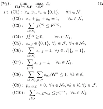
denoted asN2. The joint optimization problem is formulated
as
(P1) : min
Π,ff og,S,P maxn∈N Tn (12)
s.t.(C1) : xn, yn, zn∈ {0,1}, ∀n∈ N, (C2) : xn+yn+zn= 1, ∀n∈ N, (C3) : ∑
n∈N1 ff og
n ≤Ff og,
(C4) : fnf og≥0, ∀n∈ N1,
(C5) : sn,j ∈ {0,1}, ∀j∈ J, ∀n∈ N2,
(C6) : ∑ n∈N2
sn,j = 1, ∀j∈ J |{j= 1},
(C7) : ∑ j∈J
sn,j= 1, ∀n∈ N2,
(C8) : ∑ n∈N2
∑
j∈J
sn,jWn≤1, ∀k∈ K,
(C9) : pn,k(j)≥0, ∀n∈ N2,∀k∈ K,∀j∈ J,
(C10) : ∑ j∈J
sn,jpn,j ≤pmaxn , ∀n∈ N2.
TABLE I: Notation Definitions
Symbol Definition
Tloc
n ,Tnf og, Delay of UEnin local/fog/cloud processing
Tncloud
fnloc,fnf og, Processing ability of UEn
fnc in local/fog/cloud processing
Dn,Cn,λn Data size/computation load/processing
density of the application of UEn
Ff og Total computation capability of the fog node
pmaxn The maximum transmit power of UEn
gn,k(j) Power gain of UEnon RBkin patternj
sn,j Indicator whether patternj is allocated to UEn
rn, pn Wireless transmit rate/power of UEn
Rf c
n Wired link rate of UEnbetween fog and cloud
rn,j, pn,j Transmit rate/power of UEnon patternj
rn,k(j) Transmit rate/power of UEn
pn,k(j) on RBkin patternj
S,P RB Pattern/power allocation matrix
xn,yn,zn Offloading decisions of UEn
Π Matrix of all UEs’ offloading decisions
N,N The set/number of all UEs
N1,N1 The set/number of fog-executing UEs
N2,N2 The set/number of remote-executing UEs
K, K The set/number of RBs
J,J The set/number of all feasible patterns
Wn Feasible RB pattern matrix for UE
n
I,M,γ Number of fireworks/total explosion sparks/
mutation sparks
L Number of iterations of FA
In problem(P1), (C1) and (C2) give each UEnthe restraints on its offloading decisions; (C3) shows that the total allocated computation resource should be less than the total computation capability Ff og in the fog node; (C4) indicates that the
computation resource allocated to each fog-processing UEn
be assigned to any UE that is not allocated with RB; (C7) requires that each UE can only be assigned with one pattern; (C8) guarantees that each RB is allocated to only one UE; (C9) requires the power on each RB is nonnegative; (C10) is the maximum transmit power constraint of each UE.
Proposition 1:Problem(P1)is NP-hard.
Proof: See Appendix A.
IV. BINARYTAILOREDFIREWORKSALGORITHMBASED
JOINTCOMPUTATIONOFFLOADING ANDRESOURCE
ALLOCATIONALGORITHM
Since problem (P1) is hard to solve, in this section, we decouple it into two subproblems, i.e., offloading decisions making and resource allocation, which are solved by the proposed algorithm FAJORA.
When a firework is ignited, a burst of sparks will fill the surrounding space around the firework. Inspired by the phenomenon, the authors in [24] proposed a new kind of heuristic algorithm called fireworks algorithm (FA), and have verified that it performs well in convergence speed and global searching, compared with other heuristic algorithms such as genetic algorithm (GA) [25] and particle swarm optimization algorithm (PSO) [26]. As good candidates for solving MINLP problem, heuristic algorithms have been used widely in many fields such as radio resource allocation [26] and fuzzy control [27], etc. However, to the best understanding of us, seldom have they been used efficiently in computation offloading, especially fireworks algorithm. In the following we will intro-duce Binary Tailored Fireworks Algorithm(BTFA) firstly, then we propose the general framework of our proposed FAJORA for the considered scenario.
A. Some Concepts
1) Fireworks and Sparks: Fireworks and the newly gener-ated sparks represent feasible solutions in the solution space. Specifically, a firework/spark indicates an offloading decision matrix Πin the considered problem.
2) Fitness Function and Fitness Value: Fitness values are employed to evaluate the performance of feasible solutions. We take the objective function in (P1)as the fitness function to obtain the fitness value of each firework.
3) Binary Matrix Distance: Binary matrix distance means the Manhattan distance of two binary matrixes, i.e., the sum of the distance between each element of the two matrixes. Suppose two matrixes X andY are m×n-dimensional, the distance between the two matrixes is
d(X, Y) = m
∑
i=1
n
∑
j=1
|Xi,j−Yi,j|. (13)
B. Overview of FA
The typical steps for solving a problem with FA can be summarized as follows: First, initialize a swarm of fireworks and obtain their fitness values according to the specified fitness function. Then each firework performs explosion operator to generate some explosion sparks around the firework within a certain amplitude. The number of sparks and the explosion
amplitude are obtained according to the fitness value of each firework. The better fitness value of a firework, the more explosion sparks it will produce, and the smaller amplitude will be, and vice versa. After that several Gaussian mutation sparks are generated in order to keep population diversity. Afterwards, from the population of fireworks and sparks, several individuals are picked out as the fireworks of the next iteration. The procedure of explosion, mutation and selection is repeated until the algorithm reaches convergence, or reaches the maximum iteration index. Finally, from the individuals obtained in the last iteration, the individual with the best fitness value is selected as the solution to the constructed problem.
C. Operations of BTFA
Given totalI fireworks, the major operations of the binary tailored FA are listed as follows.
1) Explosion: The number of the explosion sparks for the
ith fireworkΠi is given by
χi=ceil
M Ifmax−f(Πi) +ϵ
∑
i=1
(fmax−f(Πi)) +ϵ
, (14)
where ceil(·) is round up function, M is a parameter con-straining the total number of explosion sparks, fmax = max(f(Πi)), i = 1, ..., I is the worst fitness value among
all theI fireworks, andϵ is an extremely tiny number which is used to avoid zero-division-error.
To avoid that one firework may generate too less or too many explosion sparks, bounds are defined for eachχi, which
is given by
ˆ
χi =
round(aM), if χi< aM
round(bM), if χi> bM, a < b <1, round(si), otherwise
(15)
whereround(·)is the rounding off function,aandbare given constants, andχˆi is the number of actual generated explosion
sparks.
For firework Πi, each explosion spark is generated like
this: 1) choose β columns from the N columns randomly; 2) perform cyclic shift on each selected column; 3) the rest columns are kept unchanged.
2) Mutation: To improve the spark diversity and thereby to increase searching capability, mutation is introduced. From theIfireworks, we chooseγof them randomly, each of which will generate a mutation spark like this: 1) chooseβ columns from the N columns randomly; 2) for each of the selected column, reset it with a random feasible offloading decision; 3) the rest columns are kept unchanged.
3) Selection: After explosion and mutation, there exist three different kinds of individuals, i.e., fireworks, explosion sparks, and mutation sparks. The individual with the best fitness value is always kept as the first firework of the next generation. To keep diversity of the population, other I−1
According to (13), the binary matrix distance between an individual Πi and other individuals is given by
R(Πi) =∑
j∈K
d(Πi,Πj), (16)
whereKis the population of all current individuals including both fireworks and sparks.
Consequently, the selected probability of individual Πi is
given by
p(Πi) = ∑R(Πi)
j∈K
R(Πi). (17)
D. BTFABasedJoint ComputationOffloading andResource
Allocation Algorithm (FAJORA)
Applying the proposed binary tailored operators to tradi-tional fireworks algorithm, and adopting the same procedure with FA, we obtain BTFA. Using BTFA we can solve the original formulated problem (P1), i.e., the final offloading decision Π and the corresponding resource allocation can
be obtained. Detailed algorithm framework is called BTFA
based joint Computation offloading and resource allocation algorithm (FAJORA) and is summarized in Algorithm 1 as folllows.
Algorithm 1 FAJORA
Initialization:
1: SetN,K,Ff og,I,M,β,γ,aandb.
2: InitializeDn, Cn, fnloc, pmaxn , Rf cn , fnc of each UE. 3: GenerateIrandom fireworksΠ1, ...,ΠI in the searching
space, perform resource allocation under each firework, and obtain the fitness value of each firework.
Iteration:
4: while1 orl <=Ldo 5: fori <=I do
6: Obtain the number of explosion sparksχi according
to (14) and (15).
7: forp <=χi do
8: Perform explosion to generate explosion sparkp.
9: Perform resource allocation underp.
10: Calculate the fitness value ofp.
11: end for
12: end for
13: forj <=γ do
14: Generate mutation sparkj.
15: Perform resource allocation underj.
16: Obtain the fitness value ofj.
17: end for
18: The best individual is considered as the first firework
of the next iteration, and the other I −1 fireworks are chosen from the rest individuals according to the selected probability in (17).
19: end while
20: Among the fireworks selected in the last iteration, the one with the minimum fitness value is considered asΠ∗.
21: Output: Π∗ and corresponding resource allocation.
V. COMPUTATIONRESOURCEALLOCATION
Next we will tackle the resource allocation subproblem em-bedded in Steps 3, 9, and 15 in Algorithm 1, where both radio and computation resource allocation need to be determined. In this section, we describe how to obtain the computation resource allocation, while radio resource allocation will be presented in the next section.
After offloading decision Π has been obtained, problem
(P1)degrades to the joint optimization of allocating compu-tation resources, RB patterns, and transmit power as follows
(P2) : min
ff og,S,Pmaxn∈N Tn (18)
s.t. (C3)−(C10).
To reduce the computation complexity, we divide(P2)into two subproblems: computation resource allocation and radio resource assignment. For computation resource allocation a-mong UEs in N1, assuming the radio resource assignmentS
andPare given, we have
(P3) : min ff ognmax∈N1
(C
nyn
fnf og +Bn
)
(19)
s.t. (C3),(C4),
whereBn =Cfnlocxn n +(T
f c
n +Tnc)zn+Dn(yrnn+zn)= Drnn, n∈ N1
is a constant. Letting Cnyn
fnf og +Bn =
Cn
fnf og +Bn
≤τ, n∈ N1,
the non-smooth problem(P3)is converted to
(P4) : min
ff og,τ τ (20)
s.t. (C3), (C4),
(C16) : Cn
fnf og
+Bn ≤τ, ∀n∈ N1.
Since Cn
fnf og ≥0, thenτ−Bn≥0, so we have
0≤ Cn
τ−Bn
≤ff og
n , ∀n∈ N1. (21)
Consequently, we have
∑
n∈N1 Cn τ−Bn
≤ ∑
n∈N1
fnf og≤Ff og. (22)
In order to minimize the maximum delay among all the fog-executing UEs, the UE with the maximum delay (which is denoted by UE∗) needs to be allocated with more computation resources, so less computation resources will be left for all the other UEs (i.e., UEs in the setN1|U E∗), leading to an increase
in the delay of those UEs. Performing the above process iteratively, all the computation resources will be distributed evenly among all the fog-executing UEs in the end. Thus we have
∑
n∈N1 Cn τ−Bn
= ∑
n∈N1 ff og
n =Ff og. (23)
Thus problem(P4)can be converted to
(P5) : min
τ τ (24)
s.t. (C17) : ∑ n∈N1
Cn τ−Bn
Since the left-hand side of (C17) is a monotonic decreasing function about τ, bisection method can be used to solve problem(P5), which is detailed in Algorithm 2.
Algorithm 2 Bisection Method for Computation Resource
Allocation
Initialization:
1: Setτmin =max{B
n},τmax= ∑ n∈N1
(CnN1 Ff og +Bn
) .
2: Seti= 1 and the precisionε >0.
Iteration:
3: while1 do
4: τi= (τmin+τmax)/2.
5: if|τmax−τmin|≤εthen 6: τ∗=τi.
7: else
8: if ∑
n∈N1 Cn
τi−Bn > Ff og then
9: τmin=τi.
10: else
11: τmax=τi.
12: end if
13: end if
14: i=i+ 1.
15: end while
16: Letτ∗=τiand substituting it into (23),ff og∗is obtained. 17: Output: ff og∗.
VI. COMMUNICATIONRESOURCEASSIGNMENT
After computational resource allocation is obtained, prob-lem (P2) degrades to the joint optimization of RB pat-tern assignment and power allocation among all remote-executing UEs in N2. Denoting the RB pattern assignment
and transmit power allocation as S = {sn,j}N
2×J and
P = {pn,k(j)}N
2×K×J, then the radio resource allocation
subproblem is given by:
(P6) : min S,Pnmax∈N2
(D
n(yn+zn) rn
+Vn
)
(25)
s.t. (C5)−(C10),
where Vn = Cfnf ogyn
n +
Cnxn
floc n + (T
f c
n +Tnc)zn = Cfnf ogyn
n +
(Tf c
n + Tnc)zn is a constant. However, (P6) is still an NP-hard problem as proven in Appendix A. To make the problem tractable, we first relax each sn,j to a continuous
interval, i.e., 0 ≤ sn,j ≤ 1; then we define a new matrix
Φ = {ϕn,k(j)}N
2×K×J = {sn,jpn,k(j)}N2×K×J to replace
P = {pn,k(j)}N2×K×J. Noting Dn(yn+zn)
rn =
Dn
rn, n ∈ N2, and letting max
n∈N2
(
Dn
rn +Vn )
= τ1, we have Drnn +Vn ≤
τ1, n∈ N2, then(P6)can be rearranged as
(P7) : min
S,Φ,τ1 τ1 (26)
s.t. (C5) : 0≤sn,j≤1, ∀n∈ N2, ∀j∈ J,
(C6)−(C8),
(C9) : ϕn,k(j)≥0, ∀n∈ N2, ∀k∈ K,
(C10) : J
∑
j=1
K
∑
k=1
ϕn,k(j)≤pmaxn , ∀n∈ N2,
(C18) :rn ≥ Dn τ1−Vn
, ∀n∈ N2.
Proposition 2:Problem(P7) is jointly convex inSandΦ for givenτ1.
Proof:See Appendix B.
Since (P7) is convex, Slater’s condition [28] is met and 0 duality gap can be assured, so we can solve it employing Lagrangian dual decomposition and sub-gradient projection method [29]. Once the optimal solution {S∗,Φ∗} to(P7) is obtained, the optimal solution{S∗,P∗} to(P6)is obtained.
A. Lagrange Dual Decomposition Based RB Pattern and Power Allocation
To reduce the number of dual variables and thus to improve convergence speed, the partial Lagrange function of (P7) is given by (27), where µ = {µn} ≽ 0, n ∈ N2 and ω =
{ωn} ≽0, n∈ N2are Lagrange dual variables corresponding
to(C10)and(C18) in(P7), respectively. The Lagrange dual function is given by
D(µ,ω) = min
S,Φ,τ1∈{(C5)−(C9)}L(
S,Φ, τ1,µ,ω), (28)
which can be decomposed intoJ−1independent subproblems (except for pattern j = 1). The jth subproblem under given dual variables(µ,ω)is given as
(P8) : min sj,Φj,τ1Lj(
sj,Φj, τ1) (29)
s.t. (C5)−(C9),
where sj = {sn,j}T
N2∗1, Φj = {ϕn,k(j)}N2×K is the
sub-matrix ofSandΦ for RB pattern j, and
Lj(sj,Φj, τ1) =τ1−
∑
n∈N2 µn
K
∑
k=1
ϕn,k(j) (30)
+ ∑
n∈N2 ωn
K
∑
k=1
sn,jW0log2
(
1 + ϕn,k(j)gn,k(j) sn,j
)
.
From (P8) we know that sj contains only one nonzero binary entry, because every patternj can only be allocated to one UE as required in constraint (C6). For patternj, assuming
sn,j, n∈ N2,is known, we optimize power allocation for each
RB in patternj. Let
ξn,j=ωn K
∑
k=1
sn,jW0log2
(
1 + ϕn,k(j)gn,k(j)
sn,j
)
−
K
∑
k=1
L(S,Φ, τ1,µ,ω) (27)
=τ1+
∑
n∈N2 µn
pmaxn −
J
∑
j=1
K
∑
k=1
ϕn,k(j)
+ ∑
n∈N2 ωn
J
∑
j=1
K
∑
k=1
sn,jW0log2
(
1 + ϕn,k(j)gn,k(j)
sn,j
)
−Dn(yn+zn)
τ1−Vn
.
(P8)reduces to the following problem
(P9) : Γn,j= min
φn,k(j)
ξn,j (32)
s.t. (C8′) : ϕn,k(j)≥0, ∀n∈ N2, k∈ K.
Let ∂ξn,j
∂φn,k(j) = 0, the optimal power allocation for each RB
in pattern j is obtained as follows
p∗n,k(j)=
ϕn,k(j)
sn,j =
(
ωnW0
µnln 2
− 1
gn,k(j)
)+
, (33)
where x+ ,max{0, x}. By substituting p∗
n,k(j) in place of
φn,k(j)
sn,j in (31), we obtainΓn,j as
Γn,j=
(
ξn,j |pn,k(j)=p∗n,k(j)
)
. (34)
Performing the procedure (31)-(34) for each UE inN2, we
obtain Γj = {Γn,j}, n ∈ N2. The UEn with the minimum Γn,j, n∈ N2, is selected as the optimal UEn∗ for patternj.
We allocate pattern j to UE n∗, and sets∗n∗,j = 1. Thus, the optimal solutions∗
j ={s∗n∗,j} to thejth sub-problem in(P8) is given by
s∗n∗,j = {
1, n∗= arg min n {Γn,j}
0, otherwise . (35)
Performing the procedure (29)-(35) for every patternj∈ J, we obtain S∗={s∗1, ...s∗
J}.
B. Heuristic Algorithm to Extract the Optimal Pattern (HAEOP)
Note that in S∗, one UE may be allocated with more
than one pattern, while in the LTE-A uplink one UE can be allocated with at most one pattern (as in (C7)), and the patterns allocated to different UEs should not contain the same RBs (as in (C8)), otherwise conflict will occur. A conflict table of each RB in 4-RB case is listed below in Table II.
TABLE II: Conflict table in 4-RB case
Index of RB Corresponding conflicting patterns
1 2,6,9,11
2 3,6,7,9,10,11
3 4,7,8,9,10,11
4 5,8,10,11
We propose a heuristic algorithm calledheuristicalgorithm to extract the optimal pattern (HAEOP) for each UE to pick out the optimal pattern from their feasible patterns subjecting to constraints (C7) and (C8). It is given in Algorithm 3 and explained below.
In the sorting process (Step 4), we will give a higher priority to the UE with less feasible patterns, since UEs with
Algorithm 3 HAEOP
1: Input: The obtained S∗.
2: List the conflict table for each RB according toWn.
3: List the initial feasible pattern set for each remote-processing UE according to S∗.
4: Sort the N2 remote-processing UEs according to the
number of their initial feasible patterns. The less it is, the top the UE. If multiple UEs have the same number of feasible patterns, compare the minimum feasible pattern index. The smaller it is, the top the UE.
5: Start the first round of pattern selection among all the valid remote UEs. If a UE has no feasible pattern, it is deemed as an invalid UE, and allocate pattern j = 1 to it. If there’s only one remote UE, choose pattern j =J
as its final scheme, then break. Else, the first UE chooses the minimum pattern index from all its feasible patterns.
6: For the middle 2 ∼ (N2 − 1) UEs, perform pattern
selection according to the following rules. (i) First each UE obtains all patterns conflicting with any its previous UEs; (ii) take out all the conflict patterns from its initial feasible pattern set, and the rest constitutes its new feasible pattern set; (iii) chooses the pattern with the minimum index from its new feasible pattern set; if the set is empty, allocate pattern j= 1to the UE.
7: The last UE first performs the same procedure as the previous 2 ∼ (N2−1) UEs did to obtain its feasible
pattern set. If the set is nonempty, choose the maximum index from this set; else choose pattern j= 1.
8: Calculate the total number of occupied RBs according to the chosen pattern of each UE. If it is less than K, start the next round of pattern selection: the first UE chooses its next feasible pattern; then the rest valid UEs repeat the same procedure as Steps 6 and 7 above, until either of the following two terminal conditions are satisfied: (i) the total number of occupied RBs equals to K, then the patterns selected in this round are considered as the optimal pattern allocation scheme; or (ii) if any valid UE has no feasible pattern, then the patterns selected in the previous round are considered as the optimal scheme.
9: Output: The optimal patternS∗∗={s∗∗
n∗,j∗}.
more feasible patterns have a higher probability of finding a feasible pattern after all other UEs have performed their pattern selection.
According toWn, a pattern with a smaller index contains
less RBs. So in Steps 5-6, the first 1 ∼ (N2−1) UEs will
finding a feasible pattern. In Step 7, the last UE will choose the feasible pattern with the maximum index in order to maximize RB utilization. If any UE is left with no feasible pattern in the first round of selection, i.e., all its initial feasible patterns conflict with the chosen patterns of its previous UEs, then the UE is allocated with pattern j = 1 (no RBs) and is called an invalid UE (i.e., it fails in task offloading), otherwise it is called a valid UE.
Step 8 terminates under one of the two conditions: 1) someone is left with no feasible pattern, then the patterns of all remote-processing UEs selected in the previous round are considered as the optimal pattern allocation scheme; 2) all the
K RBs have been allocated, then the patterns selected in this round are considered as the optimal scheme. We denote the optimal pattern allocation matrix as S∗∗={s∗∗
n∗,j∗}.
After the optimal RB pattern allocationS∗∗is obtained, we
perform the optimal power allocation for each UE n∗ on the RBs in its selected pattern j∗ as follows
p∗∗n∗,k(j∗)=
{
p∗n,k(j), n=n∗ and j=j∗
0, otherwise . (36)
C. Lagrange Multipliers Update
After solving all subproblems in (P8), S and P can be obtained for givenµandω. The dual variablesµandωcan
be updated by resolving the dual problem of (P7), which is given by
(P10) : max
µ,ω D(µ,ω) (37)
s.t. µ≽0,ω≽0.
From (27) and (28), we know that(P10)is convex, because
D(µ,ω)is a linear function about the dual variablesµandω.
By utilizing sub-gradient projection method, we solve (P10) in an iterative manner to obtain dual optimum µ∗ andω∗.
Proposition 3: The sub-gradients of D(µ, ω) at the tth iteration are given in equations (38) and (39), where p∗n,k(j)
and s∗
n,j is the optimal solution to dual function (28) for a
given set of dual variables µandω. Proof: See Appendix C.
Based on (38)–(39), the Lagrange multipliers are updated with the sub-gradient projection method [30] as follows
µn(t+ 1) = [µn(t)−h(t)▽µn(t)]+, ∀n, (40) ωn(t+ 1) = [ωn(t)−j(t)▽ωn(t)]+, ∀n, (41)
where t is the iteration index; h(t) and j(t) are positive step sizes. In this paper we adopt square summable but not summable step sizes [30], where h(t) = 1/(10∗ t), and
j(t) = 1/(10−1∗t). The Lagrange multipliers are updated
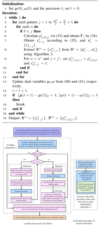
iteratively until the required precision is satisfied. The proce-dure for joint RB pattern and power allocation is summarized in Algorithm 4. For a general understanding, the work flow chart of our system is given in Fig. 2, the main body of which is our proposed FAJORA.
Algorithm 4Joint Uplink RB Pattern assignment and Power
Allocation
Initialization:
1: Set µ(0),ω(0) and the precisionδ, sett= 0.
Iteration:
2: while 1do
3: foreach pattern j= 1to K22 +K
2 + 1 do
4: foreach ndo
5: if k∈j then
6: Calculatep∗
n,k(j)via (33) and obtainΓjby (34).
7: Obtain s∗
n∗,j according to (35), and s∗j = {s∗
n∗,j}.
8: Extract S∗∗ ={s∗∗
n∗,j∗} fromS∗ ={s∗1, ...,s∗J}
using Algorithm 3.
9: Forn=n∗ andj =j∗, setp∗∗
n∗,k(j∗)=p∗n,k(j)
ands∗∗
n∗,j∗ = 1.
10: end if
11: end for
12: end for
13: Update dual variablesµ, ωfrom (40) and (41),
respec-tively.
14: t=t+ 1.
15: if ∥µ(t+ 1)−µ(t)∥2 < δ, ∥ω(t+ 1)−ω(t)∥2 < δ
then 16: break.
17: end if
18: end while
19: Output:S∗∗={s∗∗
n∗,j∗}, P∗∗={p∗∗n∗,k(j∗)}.
Initalize I offloading decision matrixes as initial fireworks
Formulate the MINLP problem of joint optimization of offloading decision, computation resource allocation, RB pattern assignment, and power allocation in a mixed fog/cloud computing LTE-A based system
Final offloading decision and the corresponding resource allocation scheme Yes
FAJORA (Algorithm 1)
Resource allocation procedure under each
firework or spark (embedded in Algorithm 1)
Bisection method based computation resource allocation (Algorithm 2)
HAEOP optimal pattern extracting for each UE (Algorithm 3, embedded
in Algorithm 4) Obtain the number of explosion
sparks of firework i according to its fitness value
Perform explosion for firework
i to generate explosion sparks
Resource allocation
i<=I ? Yes
Generate mutation sparks No
Calculate fitness value for each explosion spark
Resource allocation
Calculate fitness value for each mutation spark Iteration end?
From the set of fireworks, explosion sparks, and mutation sparks, choose I individuals as the
fireworks for the next iteration No
Among fireworks selected in the last iteration, the one with the minimum fitness value as the optimal firework (final offloading decision)
Yes
FAJORA (Algorithm 1)
i<== ?I
Yes NNo Iteration end?
No
Among fireworks selected in the last iteration, the one with the minimum fitness value as the optimal firework (final offloading decision)
Initalize I offloading decision matrixes as initial fireworks
Initialize I offloading decision matrixes as initial fireworks, perform resource allocation under each firework, and calculate the fitness value for each firework
Lagrange dual decomposition based RB
pattern and transmit power allocation
(Algorithm 4) Generate mutation sparks
Resource allocation
Calculate fitness value for each mutation spark
Mutation
From the set of fireworks, explosion sparks, and mutation sparks, choose Iindividuals as the
fireworks for the next iteration
Selection
Obtain the number of explosion sparks of firework iaccording
to its fitness value
Perform explosion for firework
ito generate explosion sparks
Resource allocation
Calculate fitness value for each explosion spark
Explosion
(a) Main framework of FAJORA
(b) Detailed procedure of resource allocation
Fig. 2:The work flow chart of our system.
VII. COMPLEXITYANALYSIS
▽µn(t) =pmaxn − J
∑
j=1
s∗n,jp∗n,j, (38)
▽ωn(t) = J
∑
j=1
s∗n,jrn,j−
Dn(yn+zn) τ1−Vn
= J
∑
j=1
K
∑
k=1
s∗n,jW0log2
(
1 +p∗n,k(j)gn,k(j)
)
−Dn(yn+zn)
τ1−Vn
, (39)
procedure is performed
I
∑
i=1
iχi times for the I
∑
i=1
iχi
explo-sion sparks, respectively. In Step 15, the resource allocation procedure is performed γ times for the γ mutation sparks, respectively. For notational simplicity, we define the total
number of explosion and mutation sparks asΞ = ∑I
i=1
iχi+γ.
In each resource allocation procedure, computation sources are allocated using Algorithm 2, and then radio re-sources are allocated employing Algorithm 4. In Algorithm 2, it requiresO(log2
(
τmax−τmin
ε
))
iterations for the bisection method to converge.
In Algorithm 4, the complexity mainly comes from the extracting of RB pattern in Step 8, i.e., Algorithm 3. The sub-gradient projection method in the outer ’while’ loop that needs O(1
δ2
)
iterations to converge [28], the K22 + K
2 + 1
iterations in the outer ’for’ loop, and the at mostN iterations in the inner ’for’ loop. The complexity of Algorithm 3 mainly comes form the pattern extracting procedure in its Steps 5– 8. Since there are at most N2 =N remote-processing UEs,
the complexity of the first round of RB pattern extracting in Steps 5–7 is O(N). Assuming that the first remote-processing UE possesCfeasible patterns, since all the remote-processing UEs are sorted according to the ascending order of their number of feasible patterns, C is far less than N, and thus the complexity of RB pattern extracting in Steps 5–8 is O(CN) = O(N). Consequently, the complexity of Algorithm 3 is O(N). Hence, the complexity of Algorithm 4 is O(1
δ2 ∗(K 2
2 +
K
2 + 1)∗N∗N
)
=O(1
δ2K2N2
) . There-fore, the complexity of each resource allocation procedure is
O(log2
(
τmax−τmin
ε
))
+O(1
δ2K2N2
)
=O(1
δ2K2N2
) . Based on the above analysis and given that the outer ’while’ loop in Algorithm 1 runs for L times, the complexity of FAJORA isO(1
δ2ΞLK2N2
) .
VIII. RESULTS ANDDISCUSSIONS
In this section, simulation results are presented to evaluate the performance of the proposed algorithms. The following parameters remain unchanged through our simulations: L = 20,K= 15[9], W0= 180KHz [9],pmaxn = 2 W [22].
The following parameters are set as default unless otherwise specified: N = 6,I = 2, M = 4, γ = 1, a= 0.2, b= 0.8,
Ff og= 5∗109cycles/s [18],fc
n= 20∗109cycles/s [16],fnloc
is uniformly distributed in [50,400] M cycles/s, and Rf c
n =
15∗106 b/s [20]. For simplicity, the wireless channel gain
gn,k(j)=
hn,k(j)
σ2 is assumed to take values in[5,14]randomly
[29]. We adopt face recognition [12] as the default application, whereDn= 0.42MB and λn = 297.62cycles/bit [12].
Next, we verify the performance gain obtained by our proposed algorithms and the following schemes are compared.
• The proposed scheme (FAJORA): The scheme obtains offloading decisions and resource allocation using FAJO-RA in Algorithm 1, where in each iteration computation resource is allocated using Algorithm 2, RB pattern and power are allocated using Algorithm 4, and each UE picks out the optimum RB pattern using Algorithm 3.
• Radio andcomputationresourceallocation optimization (RCRA): RB pattern and power are allocated using Al-gorithms 3 and 4, computation resource are allocated using Algorithm 2, and offloading decisions are obtained randomly.
• Radio resource allocation with HAEOP (RRA-H): RB pattern and power are allocated employing Algorithms 3 and 4, while offloading decisions and computation resource allocation are obtained randomly.
• Radioresourceallocation andrandom pattern extracting (RRA-R): RB pattern and power are allocated using Algorithm 4, and from the allocated patterns each UE selects one of which randomly. Offloading decisions and computation resource allocation are obtained randomly. • Local processing (Local): All UEs process their
applica-tions locally without optimization.
Moreover, in the following Figs. 8 and 9, another algo-rithm namedSDRbasedoffloadingdecision optimization and optimized resource allocation algorithm (SDR-ODRA) was considered as a benchmark to demonstrate the performance of our proposed BTFA based offloading decision making algo-rithm. In SDR-ODRA, the offloading decisions are obtained using the SDR based algorithm in [20], where in each iteration computation resource is allocated using Algorithm 2, RB pattern and power are allocated using Algorithm 4, and each UE picks out the optimum RB pattern using Algorithm 3.
Remark: SDR based offloading decision making algorithm was first novelly proposed by the authors in [20], and now has been widely used in many existing works. Similar to our previous work [23], the number of runs (i.e., randomization trails) [23] in SDR-ODRA is set as 6.
Five metrics are adopted, including: 1) three kinds of delay, i.e., the maximum, minimum and average delay of all UEs, which are denoted as Tmax (i.e., objective value),Tmin, and Tav, respectively; 2) the number of benefited UEs, where
A. Convergence of Algorithms 1, 2 and 4
0 10 20 30 40 50
3.5 4 4.5 5 5.5 6 6.5 7
Number of iterations
Objective value (s)
Fig. 3:Convergence of Algorithm 1 (FAJORA).
0 2 4 6 8 10 12
0 1 2 3 4 5 6 7 8
Number of iterations
ζ1
Ffog=1*109 Ffog=3*109 Ffog=5*109 Ffog=8*109
Fig. 4:Convergence of Algorithm 2.
0 5 10 15 20
0 5 10 15x 10
10
Dual variables
µn
µ1 µ2 µ3 µ4
0 5 10 15 20
0 2 4 6x 10
7
Number of iterations
Dual variables
ωn
ω1 ω2 ω3 ω4
Fig. 5:Convergence of Algorithm 4.
Fig. 3 verifies the convergence of the outer loop of FAJORA in Algorithm 1, from which we can see FAJORA converges fast within 10 iterations. Figs. 4 and 5 evaluate the convergence rate of the main loop of Algorithms 2 and 4, respectively, both of which are embedded in Steps 3, 9 and 15 in Algorithm 1. As discussed in Section V, τ is the maximum delay of all
fog-processing UEs, and Fig. 4 shows thatτ decreases under different Ff og after each iteration until convergence. Fig. 5
shows that the dual variables in Algorithm 4 converge fast. According to the three figures, we know that the proposed algorithms are cost-efficient in solving the NP-hard problem
(P1).
1 2 3 4 5
1 1.5 2 2.5 3 3.5
Number of UEs (a)
Objective value T
max
(s)
FAJORA Exhaustive
1 2 3 4 5
0 100 200 300 400 500 600
Number of UEs (b)
Execution time of algorithm (s)
FAJORA Exhaustive
Fig. 6:Effectiveness and complexity of FAJORA.
Fig. 6 shows the comparisons in effectiveness and com-plexity between the proposed algorithm FAJORA and ex-haustive algorithm, where offloading decisions are obtained by exhaustive search, and computation and communication resource allocation employ our proposed Algorithms 2, 3, and 4. From the Fig. 6(a), it can be known that FAJORA is slightly inferior to exhaustive search in performance, i.e., a little increase in objective value. However, the complexity comparison in Fig. 6(b) indicates that the execution time of exhaustive algorithm increases exponentially with the number of UEs, while FAJORA only takes a little execution time even with more UEs, indicating that is good in scalability.
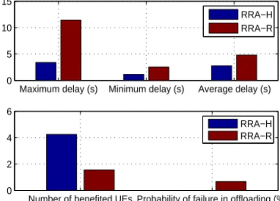
B. Effectiveness of Algorithm 3 (HAEOP)
Maximum delay (s) Minimum delay (s) Average delay (s) 0
5 10 15
RRA−H RRA−R
Number of benefited UEs Probability of failure in offloading (%) 0
2 4 6
RRA−H RRA−R
Fig. 7:Performance evaluation of Algorithm 3.
are always much shorter than that of RRA-R. The second sub-figure indicates RRA-H could benefit more UEs and reduce the probability of failures in offloading effectively.
The reason for Fig. 7 is that: in RRA-R, each UE selects a random pattern from its feasible patterns, thus its chosen pat-tern may contain the same RB with the patpat-terns chosen by its previous UEs, and consequently conflict will happen, leading to higher failure probability and less benefited UEs. While in RRA-H, since HAEOP is adopted in pattern selection, each UE picks out the optimum feasible pattern, considering exclu-siveness of RBs, thus failures could be avoided effectively, and therefore more UEs will be benefited as is shown in the second sub-figure. On the other hand, HAEOP takes RB utilization into account, thus the maximum RB utilization can be obtained under the final selected pattern allocation scheme. Consequently,Tmax,TminandTav can be reduced greatly as
shown in the first sub-figure.
C. Performance Comparisons versus Different Application parameters
0 50 100 150 200 250 300 350 400 0
2 4 6 8 10 12 14
Processing density λ
n (CPU cycles/bit)
Objective value T
max
(s)
FAJORA SDR−ODRA RRA−H RCRA RRA−R Local
Fig. 8:Objective valueTmaxcomparison under different processing
densityλn.
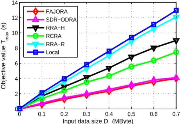
0 0.1 0.2 0.3 0.4 0.5 0.6 0.7 0
2 4 6 8 10 12 14
Input data size Dn (MByte)
Objective value T
max
(s)
FAJORA SDR−ODRA RRA−H RCRA RRA−R Local
Fig. 9:Objective valueTmaxcomparison under different input data
sizeDn.
Figs. 8 and 9 shows how application parameters including processing density λn and input data size Dn affect the
objective value Tmax, respectively. The two figures are in
accordance with our intuition that more input data Dn or
the higher computation complexity λn, higher delay will be
brought in, and consequently a lager value ofTmax. Moreover,
as a joint optimization of offloading decisions and resource allocation, FAJORA performs always the best, followed by SDR-ODRA, RCRA, RRA-H, and RRA-R successively, and Local is the worst in performance.
However, some differences exist between the two figures. In Fig. 8,Dntakes the default value 0.42 MB, which is relatively
large. When λn is very small, local processing is usually a
good choice, while offloading will consume more time in data transmission. In Fig. 9,λn = 297.62cycles/bit. When Dn is
very small, the computation workloadCnis also very small, so
all the algorithms will consumes quite less time, and therefore
Tmax is very small for all the algorithms.
It should be noted that, although SDR-ODRA can obtain almost the same performance as FAJORA, the computational complexity of SDR-ODRA is much higher than FAJORA in the offloading decision making process. In SDR-ODRA, of-floading decisions are obtained using CVX and randomization, where interior point method is adopted, leading to higher complexity. In FAJORA, the outer fireworks algorithm need several iterations to converge, and in each iteration each spark (i.e., an offloading decision) can be generated using fireworks operators with very tiny complexity.
D. Performance Comparisons versus Channel State
0.5~2 4~6 8~10 12~14 16~18 0
2 4 6 8 10 12 14
Wireless channel gain g
n,k(j)
Objective value (s)
FAJORA RRA−H RCRA RRA−R Local
Fig. 10:Objective valueTmax comparison under different different
wireless channel gaingn,k(j).
Figs. 10 and 11 display how channel state affects the objective value Tmax, including the wireless access channel
gain gn,k(j) between UEs and the fog node, and the wired
link rateRf c
n between fog and cloud, respectively. As channel
state has no influence on local processing, its objective value always keeps still. However, when the channel state gets better and better, less time will be consumed in data transmission for all other algorithms, leading to a decrease inTmax for them.
From the two figures we can also find that FAJORA always performs the best, with its objective valueTmax far less than
1 3 5 10 15 20 0
2 4 6 8 10 12
Wired rate R
n fc
between fog and cloud (Mbit/s)
Objective value (s)
FAJORA RRA−H RCRA RRA−R Local
Fig. 11:Objective valueTmaxcomparison under different different
wired rate Rf c
n between fog and cloud.
50 100 150 200 250 300 350 400 0
5 10 15 20 25
Computation capabicity fnloc of UE (M cycles/s)
Objective value T
max
(s)
FAJORA RRA−H RCRA RRA−R Local
Fig. 12: Objective value Tmax comparison under different local
processing capabilityfnloc.
E. Performance Comparisons versus the Processing Capabil-ities
The impact of local processing capability floc
n onTmax is
shown in Fig. 12, where Tmax decreases quickly with the
increase of floc
n for all the algorithms. When the value of floc
n is large, Local performs the best in delay reduction.
This is reasonable, because when the processing capability of a UE is strong enough, it is capable in processing most applications with good performance, and there’s no need to offload. However, the obtained Tmax of FAJORA is only a
little higher than Local, indicating FAJORA performs well in this case. On the other hand, when floc
n is very small,
FAJORA still performs very well, whereas the delay of all other algorithms are too long to bear.
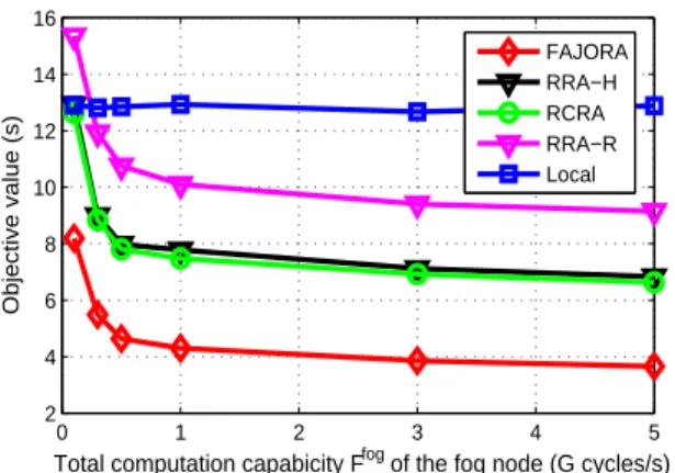
In Figs. 13 and 14, we evaluate the impact of the fog processing capability Ff og and cloud processing ability fc n
on Tmax. When either of the two parameters increase, Tmax
decrease, which is the same for all the algorithms (except for Local) and is in line with our intuition. Besides, FAJORA performs the best in delay reduction and far outdistances other algorithms.
0 1 2 3 4 5
2 4 6 8 10 12 14 16
Total computation capabicity Ffog of the fog node (G cycles/s)
Objective value (s)
FAJORA RRA−H RCRA RRA−R Local
Fig. 13:Objective valueTmax comparison under different total fog
processing capabilityFf og.
0 5 10 15 20
0 5 10 15 20
Computation capabicity f
n c
of the cloud server (G cycles/s)
Objective value (s)
FAJORA RRA−H RCRA RRA−R Local
Fig. 14: Objective value Tmax comparison under different cloud
processing capabilityfc
n.
I=1,U=2 I=2,U=4 I=3,U=6 I=4,U=8 I=5,U=10 0
0.5 1 1.5 2 2.5 3 3.5 4
Number of fireworks I and sparks U
Three different delay metrics (s)
T
max Tmin Tav
Fig. 15: Objective valueTmax comparison under different number
F. Performance Comparisons versus FA’s Parameters
Fig. 15 presents the influence of the parameters in fireworks algorithm on three different delay metrics Tmax, Tmin and Tav. For notational simplicity, we define the total number of
explosion and mutation sparks as U = ∑I
i=1
iχi +γ. As is
shown, with the number of fireworksIand sparksU increase, the three delays all decrease. This is because, as was men-tioned, each of the fireworks or sparks is an offloading decision matrix and corresponds to a resource allocation scheme. So the more fireworks and sparks, the more joint computation offloading and resource allocation schemes, consequently the better searching capabilities and the shorter obtained delays. However, the more fireworks and sparks, the more computation complexity, whereas the delay reduction is not so significantly as is shown in Fig. 15. Thus we choose I = 2 and U = 4
as the default number of fireworks and sparks, respectively, to strike a balance between searching capability and computation complexity.
IX. CONCLUSIONS
In this paper, we have proposed a framework to optimize computation offloading, computation resource allocation, RB pattern assignment, and transmit power allocation. In the optimization framework, we have considered the maximum delay reduction problem, which was modeled as an MINLP problem. We have proposed a low-complexity general al-gorithm framework FAJORA to decompose it into several subproblems, where offloading decisions was obtained within the main framework of FAJORA, and computation and radio resources allocation was solved by the embedded Algorithms 2, 3, and 4. Abundant simulation results have demonstrated the convergence and effectiveness of our proposed algorithms.
APPENDIXA
PROOF OFPROPOSITION1
Proof: In problem (P1), there are four sets of mutually coupled variables to be optimized. If the optimal offloading decision Π∗ and computation resource allocation ff og∗ are
given, then (P1) reduces to the joint optimization of RB pattern assignment and transmit power control among all the remote-processing UEs in N2. If the optimal RB pattern
assignment S∗ is also obtained, then the problem can be
further reduced to
(P1
1) : min P nmax∈N2
(D
n rn
+Vn
)
(42)
s.t. (C9) :pn,k(j)≥0,∀n∈ N2,∀k∈ K,∀j∈ J,
(C10) :∑ j∈J
∑
k∈K
pn,k(j)≤pmaxn ,∀n∈ N2,
whereVn=Cfnf ogyn
n +
Cnxn
floc n + (T
f c
n +Tnc)zn= Cfnf ogyn n + (T
f c n + Tc
n)zn is a constant, so problem (P11)is equivalent to
(P2
1) : min P nmax∈N2
Dn rn
(43)
s.t. (C9),(C10).
In the following, we show that problem(P2
1)is NP-hard. As a special case, we assume there is no max
n∈N2
operation, then
problem(P2
1)becomes
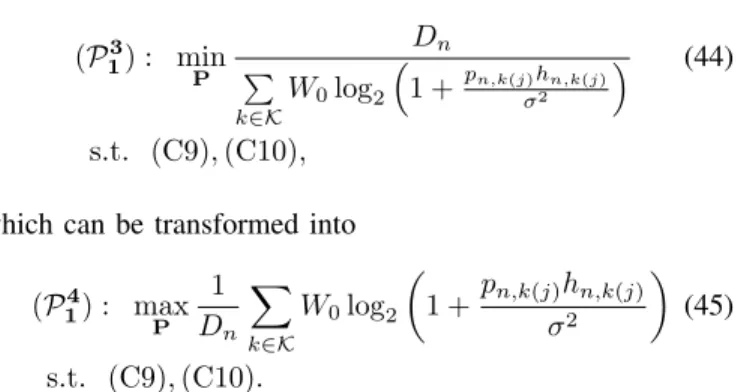
(P3
1) : min P
Dn
∑
k∈K
W0log2
(
1 + pn,k(j)hn,k(j) σ2
) (44)
s.t. (C9),(C10),
which can be transformed into
(P4
1) : max P
1
Dn
∑
k∈K
W0log2
(
1 +pn,k(j)hn,k(j)
σ2
) (45)
s.t. (C9),(C10).
We can see that the objective function in(P4
1)is a sigmoidal function.
Definition: A continuous function f[l, u] → R is defined as a sigmoidal if: either it is convex, concave, or convex for
x≤z, z∈[l, u]and concave forx≥z[31], [32]. Since all the constraints of(P4
1)are linear,(P 4
1)maximizes the sum of a set of sigmoidal functions over a convex set, which is a sigmoidal programming problem and is NP-hard [31], [32]. Consequently, problem(P1)is NP-hard, and Proposition 1 holds.
APPENDIXB
PROOF OFPROPOSITION2
Proof: When f(x) is concave, then the perspective function g(x, t) = tf(x/t) is concave, too [28]. Since
sn,jlog2(1 +
φn,k(j)gn,k(j)
sn,j ) is the perspective function of the concave function log2(1 + ϕn,k(j)gn,k(j)), it preserves
concavity, too. As the sum of several concave functions is still
concave,
J
∑
j=1
K
∑
k=1
sn,jlog2(1 +
φn,k(j)gn,k(j)
sn,j )is also concave. On the other hand, the super-level set of concave function is convex [28], so(C18) is convex. Moreover,(C5)−(C10)
are all linear constraints. Thus,(P7)is a convex optimization programming that minimize a convex function over a convex set.
APPENDIXC
PROOF OFPROPOSITION3
Proof: Observing the definition of D(µ,ω)of (28), we have
D(µ′,ω′)≥τ1+
∑
n∈N2 µ′n
pmaxn −
J
∑
j=1
K
∑
k=1
ϕ∗n,k(j)
+
∑
n∈N2 ωn′
J
∑
j=1
K
∑
k=1
W0s∗n,jlog2(1+
ϕ∗
n,k(j)gn,k(j)
s∗
n,j
)−Dn(yn+zn)
τ1−Vn