Combinatorics

(1)

Combinatorics

an upper-level introductory course

in enumeration, graph theory, and design theory

by

Joy Morris

University of Lethbridge

Version 1.1 of June 2017

(2)

[email protected]

c

2014–2017 by Joy Morris. Some rights reserved.

You are free to copy this book, to distribute it, to display it, and to make derivative works, under the following conditions: (1) Attribution. You must give the original author credit. (2) Noncommercial. You may not use this work for commercial purposes. (3) Share Alike. If you alter, transform, or build upon this work, you may distribute the resulting work only under a license identical to this one. — For any reuse or distribution, you must make clear to others the license terms of this work. Any of these conditions can be waived if you get permission from the copyright holder. Your fair use and other rights are in no way affected by the above. — This is a human-readable summary of the full license, which is available on-line at

(3)

Part II.

Graph Theory

Chapter 11. Basics of Graph Theory 86 §11A. Background . . . 86

§11B. Basic definitions, terminology, and notation - - - 87

§11C. Deletion, complete graphs, and the Handshaking Lemma . . . 90

§11D. Graph isomorphisms - - - 92

Summary . . . 98

Chapter 12. Moving through graphs 99 §12A. Directed graphs . . . 99

§12B. Walks and connectedness - - - 100

§12C. Paths and cycles . . . .102

§12D. Trees - - - 105

Summary . . . .108

Chapter 13. Euler and Hamilton 109 §13A. Euler tours and trails . . . .109

§13B. Hamilton paths and cycles - - - 113

(5)

iii

Chapter 14. Graph Colouring 119

§14A. Edge colouring . . . .119

§14B. Ramsey Theory - - - 125

§14C. Vertex colouring . . . .129

Summary - - - 133

Chapter 15. Planar graphs 134 §15A. Planar graphs . . . .134

§15B. Euler’s Formula - - - 139

§15C. Map colouring . . . .144

Summary - - - 148

Part III.

Design Theory

Chapter 16. Latin squares 150 §16A. Latin squares and Sudokus . . . .150

§16B. Mutually orthogonal Latin squares (MOLS) - - - 151

§16C. Systems of distinct representatives . . . .157

Summary - - - 162

Chapter 17. Designs 163 §17A. Balanced Incomplete Block Designs (BIBD) . . . .163

§17B. Constructing designs, and existence of designs - - - 166

§17C. Fisher’s Inequality . . . .169

Summary - - - 172

Chapter 18. More designs 173 §18A. Steiner and Kirkman triple systems . . . .173

§18B. t-designs - - - 178

§18C. Affine planes . . . .181

§18D. Projective planes - - - 187

Summary . . . .188

Chapter 19. Designs and Codes 189 §19A. Introduction . . . .189

§19B. Error-correcting codes - - - 190

§19C. Using the generator matrix for encoding . . . .193

§19D. Using the parity-check matrix for decoding - - - 195

§19E. Codes from designs . . . .199

Summary - - - 201

Index 202

List of Notation 204

(6)

(7)

Chapter 1

What is

Combinatorics?

Combinatorics is a subfield of “discrete mathematics,” so we should begin by asking what discrete mathematics means. The differences are to some extent a matter of opinion, and various mathematicians might classify specific topics differently.

“Discrete” should not be confused with “discreet,” which is a much more commonly-used word. They share the same Latin root, “discretio,” which has to do with wise discernment or separation. In the mathematical “discrete,” the emphasis is on separateness, so “discrete” is the opposite of “continuous.” If we are studying objects that can be separated and treated as a (generally countable) collection of units rather than a continuous structure, then this study falls into discrete mathematics.

In calculus, we deal with continuous functions, so calculus is not discrete mathematics. In linear algebra, our matrices often have real entries, so linear algebra also does not fall into discrete mathematics.

Text books on discrete mathematics often include some logic, as discrete mathematics is often used as a gateway course for upper-level math. Elementary number theory and set theory are also sometimes covered. Algorithms are a common topic, as algorithmic techniques tend to work very well on the sorts of structures that we study in discrete mathematics.

In Combinatorics, we focus on combinations and arrangements of discrete structures. There are five major branches of combinatorics that we will touch on in this course: enumeration, graph theory, Ramsey Theory, design theory, and coding theory. (The related topic of cryptog-raphy can also be studied in combinatorics, but we will not touch on it in this course.) We will focus on enumeration, graph theory, and design theory, but will briefly introduce the other two topics.

1A. Enumeration

Enumeration is a big fancy word for counting. If you’ve taken a course in probability and statistics, you’ve already covered some of the techniques and problems we’ll be covering in this course. When a statistician (or other mathematician) is calculating the “probability” of a particular outcome in circumstances where all outcomes are equally likely, what they usually do is enumerate all possible outcomes, and then figure out how many of these include the outcome they are looking for.

EXAMPLE 1.1.What is the probability of rolling a 3 on a 6-sided die?

SOLUTION.To figure this out, a mathematician would count the sides of the die (there are six) and count how many of those sides display a three (one of them). She would conclude that the probability of rolling a 3 on a 6-sided die is 1/6 (one in six).

(8)

That was an example that you could probably figure out without having studied enumera-tion or probability, but it nonetheless illustrates the basic principle behind many calculaenumera-tions of probability. The object of enumeration is to enable us to count outcomes in much more complicated situations. This sometimes has natural applications to questions of probability, but our focus will be on the counting, not on the probability.

After studying enumeration in this course, you should be able to solve problems such as:

•If you are playing Texas Hold’em poker against a single opponent, and the two cards in your hand are a pair, what is the probability that your opponent has a higher pair?

•How many distinct Shidokus (4-by-4 Sudokus) are there?

•How many different orders of five items can be made from a bakery that makes three kinds of cookies?

•Male honeybees come from a queen bee’s unfertilised eggs, so have only one parent (a female). Female honeybees have two parents (one male, one female). Assuming all ancestors were distinct, how many ancestors does a male honeybee have from 10 generations ago?

Although all of these questions (and many others that arise naturally) may be of interest to you, the reason we begin our study with enumeration is because we’ll be able to use many of the techniques we learn, to count the other structures we’ll be studying.

1B. Graph Theory

When a mathematician talks about graph theory, she is not referring to the “graphs” that you learn about in school, that can be produced by a spreadsheet or a graphing calculator. The “graphs” that are studied in graph theory are models of networks.

Any network can be modeled by using dots to represent the nodes of the network (the cities, computers, cell phones, or whatever is being connected) together with lines to represent the connections between those nodes (the roads, wires, wireless connections, etc.). This model is called a graph. It is important to be aware that only at a node may information, traffic, etc. may pass from one edge of a graph to another edge. If we want to model a highway network using a graph, and two highways intersect in the middle of nowhere, we must still place a node at that intersection. If we draw a graph in which edges cross over each other but there is no node at that point, you should think of it as if there is an overpass there with no exits from one highway to the other: the roads happen to cross, but they are not connecting in any meaningful sense.

EXAMPLE 1.2.The following diagram:

Fort Macleod Lethbridge Medicine Hat Calgary

Strathmore

is a graph.

(9)

1. What is Combinatorics? 3

be scheduled at the same time, or some nodes might represent students and others classes, with a line between a student and each of the classes he or she is taking).

After studying graph theory in this course, you should be able to solve problems such as:

•How can we find a good route for garbage trucks to take through a particular city?

•Is there a delivery route that visits every city in a particular area, without repetition?

•Given a collection of project topics and a group of students each of whom has expressed interest in some of the topics, is it possible to assign each student a unique topic that interests him or her?

•A city has bus routes all of which begin and end at the bus terminal, but with different schedules, some of which overlap. What is the least number of buses (and drivers) required in order to be able to complete all of the routes according to the schedule?

•Create a schedule for a round-robin tournament that uses as few time slots as possible. Some of these questions you may only be able to answer for particular kinds of graphs.

Graph theory is a relatively “young” branch of mathematics. Although some of the problems and ideas that we will study date back a few hundred years, it was not until the 1930s that these individual problems were gathered together and a unified study of the theory of graphs began to develop.

1C. Ramsey Theory

Ramsey theory takes its name from Frank P. Ramsey, a British mathematician who died in 1930 at the tragically young age of 26, when he developed jaundice after an operation.

Ramsey was a logician. A result that he considered a minor lemma in one of his logic papers now bears the name “Ramsey’s Theorem” and was the basis for this branch of mathematics. Its statement requires a bit of graph theory: givenc colours and fixed sizesn1, . . . , nc, there is

an integer r=R(n1, . . . , nc) such that for any colouring the edges of of a complete graph onr

vertices, there must be some ibetween 1 and c such that there is a complete subgraph on ni

vertices, all of whose edges are coloured with colouri.

In addition to requiring some graph theory, that statement was a bit technical. In much less precise terms that don’t require so much background knowledge (but could be misleading in specific situations), Ramsey Theory asserts that if structure is big enough and contains a property we are interested in, then no matter how we cut it into pieces, at least one of the pieces should also have that property. One major theorem in Ramsey Theory is van der Waerden’s Theorem, which states that for any two constants c and n, there is a constant V(c, n) such that if we take V(c, n) consecutive numbers and colour them with c colours, there must be an arithmetic progression of length nall of whose members have been coloured with the same colour.

EXAMPLE 1.3.Here is a small example of van der Waerden’s Theorem. With two colours and a desired length of 3 for the arithmetic progression, we can show that V(2,3) > 8 using the following colouring:

3 4 5 6 7 8 9 10

(In case it is difficult to see, we point out that 3, 4, 7, and 8 are black, while 5, 6, 9, and 10 are grey, a different colour.) Notice that with eight consecutive integers, the difference in a three-term arithmetic progression cannot be larger than three. For every three-term arithmetic progression with difference of one, two, or three, it is straightforward to check that the numbers have not all received the same colour.

(10)

We will touch lightly on Ramsey Theory in this course, specifically on Ramsey’s Theorem itself, in the context of graph theory.

1D. Design Theory

Like graph theory, design theory is probably not what any non-mathematician might expect from its name.

When researchers conduct an experiment, errors can be introduced by many factors (in-cluding, for example, the timing or the subject of the experiment). It is therefore important to replicate the experiment a number of times, to ensure that these unintended variations do not account for the success of a particular treatment. If a number of different treatments are being tested, replicating all of them numerous times becomes costly and potentially infeasible. One way to reduce the total number of trials while still maintaining the accuracy, is to test multiple treatments on each subject, in different combinations.

One of the major early motivations for design theory was this context: given a fixed number of total treatments, and a fixed number of treatments we are willing to give to any subject, can we find combinations of the possible treatments so that each treatment is given to some fixed number of subjects, and any pair of treatments is given together some fixed number of times (often just once). This is the basic structure of a block design.

EXAMPLE 1.4.Suppose that we have seven different fertilisers and seven garden plots on which to try them. We can organise them so that each fertiliser is applied to three of the plots, each garden plot receives 3 fertilisers, and any pair of fertilisers is used together on precisely one of the plots. If the different fertilisers are numbered one through seven, then a method for arranging them is to place fertilisers 1, 2, and 3 on the first plot; 1, 4, and 5 on the second; 1, 6, and 7 on the third; 2, 4, and 6 on the fourth; 2, 5, and 7 on the fifth; 3, 4, and 7 on the sixth; and 3, 5, and 6 on the last. Thus,

123 145 167 246 257 347

356

is a design.

This basic idea can be generalised in many ways, and the study of structures like these is the basis of design theory. In this course, we will learn some facts about when designs exist, and how to construct them.

After studying design theory in this course, you should be able to solve problems such as: Is it possible for a design to exist with a particular set of parameters?

What methods might we use in trying to construct a design?

1E. Coding Theory

In many people’s minds “codes” and “cryptography” are inextricably linked, and they might be hard-pressed to tell you the difference. Nonetheless, the two topics are vastly different, as is the mathematics involved in them.

(11)

1. What is Combinatorics? 5

Codes are used for many purposes in which the information is not intended to be secret. For example, computer programs are transformed into long strings of binary data, that a computer reinterprets as instructions. When you text a photo to a friend, the pixel and colour information are converted into binary data to be transmitted through radio waves. When you listen to an .mp3 file, the sound frequencies of the music have been converted into binary data that your computer decodes back into sound frequencies.

Electronic encoding is always subject to interference, which can cause errors. Even when a coded message is physically etched onto a device (such as a dvd), scratches can make some parts of the code illegible. People don’t like it when their movies, music, or apps freeze, crash, or skip over something. To avoid this problem, engineers use codes that allow our devices to automatically detect, and correct, minor errors that may be introduced.

In coding theory, we learn how to create codes that allow for error detection and correction, without requiring excessive memory or storage capacity. Although coding theory is not a focus of this course, designs can be used to create good codes. We will learn how to make codes from designs, and what makes these codes “good.”

EXAMPLE 1.5.Suppose we have a string of binary information, and we want the computer to store it so we can detect if an error has arisen. There are two symbols we need to encode: 0 and 1. If we just use 0 for 0 and 1 for 1, we’ll never know if a bit has been flipped (from 0 to 1 or vice versa). If we use 00 for 0 and 01 for 1, then if the first bit gets flipped we’ll know there was an error (because the first bit should never be 1), but we won’t notice if the second was flipped. If we use 00 for 0 and 11 for 1, then we will be able to detect an error, as long as at most one bit gets flipped, because flipping one bit of either code word will result in either 01 or 10, neither of which is a valid code word. Thus, this code allows us to detect an error. It does not allow us to correct an error, because even knowing that a single bit has been flipped, there is no way of knowing whether a 10 arose from a 00 with the first bit flipped, or from a 11 with the second bit flipped. We would need a longer code to be able to correct errors.

After our study of coding theory, you should be able to solve problems such as:

•Given a code, how many errors can be detected?

•Given a code, how many errors can be corrected?

•Construct some small codes that allow detection and correction of small numbers of errors.

EXERCISES 1.6.Can you come up with an interesting counting problem that you wouldn’t know how to solve?

SUMMARY:

•enumeration

•graph theory

•Ramsey theory

•design theory

(12)

(13)

Part I

(14)

Basic Counting

Techniques

When we are trying to count the number of ways in which something can happen, sometimes the answer is very obvious. For example, if a doughnut shop has five different kinds of doughnuts for sale and you are planning to buy one doughnut, then you have five choices.

There are some ways in which the situation can become slightly more complicated. For example, perhaps you haven’t decided whether you’ll buy a doughnut or a bagel, and the store also sells three kinds of bagels. Or perhaps you want a cup of coffee to go with your doughnut, and there are four different kinds of coffee, each of which comes in three different sizes.

These particular examples are fairly small and straightforward, and you could list all of the possible options if you wished. The goal of this chapter is to use simple examples like these to demonstrate two rules that allow us to count the outcomes not only in these situations, but in much more complicated circumstances. These rules are the product rule, and thesum rule.

2A. The product rule

The product rule is a rule that applies when we there is more than one variable (i.e. thing that can change) involved in determining the final outcome.

EXAMPLE 2.1. Consider the example of buying coffee at a coffee shop that sells four varieties and three sizes. When you are choosing your coffee, you need to choose both variety and size. One way of figuring out how many choices you have in total, would be to make a table. You could label the columns with the sizes, and the rows with the varieties (or vice versa, it doesn’t matter). Each entry in your table will be a different combination of variety and size:

Small Medium Large

Latte small latte medium latte large latte

Mocha small mocha medium mocha large mocha

Espresso small espresso medium espresso large espresso Cappuccino small cappuccino medium cappuccino large cappuccino

[image:14.612.116.479.560.628.2]

As you can see, a different combination of variety and size appears in each space of the table, and every possible combination of variety and size appears somewhere. Thus the total number of possible choices is the number of entries in this table. Although in a small example like this we could simply count all of the entries and see that there are twelve, it will be more useful to notice that elementary arithmetic tells us that the number of entries in the table will be the number of rows times the number of columns, which is four times three.

In other words, to determine the total number of choices you have, we multiply the number of choices of variety (that is, the number of rows in our table) by the number of choices of size

(15)

2. Basic Counting Techniques 9

(that is, the number of columns in our table). This is an example of what we’ll call theproduct rule.

We’re now ready to state the product rule in its full generality.

THEOREM 2.2. Product Rule Suppose that when you are determining the total number of outcomes, you can identify two different aspects that can vary. If there aren1 possible outcomes for the first aspect, and for each of those possible outcomes, there are n2 possible outcomes for the second aspect, then the total number of possible outcomes will ben1n2.

In the above example, we can think of the aspects that can change as being the variety of coffee, and the size. There are four outcomes (choices) for the first aspect, and three outcomes (choices) for the second aspect, so the total number of possible outcomes is 4·3 = 12.

Sometimes it seems clear that there are more than two aspects that are varying. If this happens, we can apply the product rule more than once to determine the answer, by first identifying two aspects (one of which may be “all the rest”), and then subdividing one or both of those aspects. An example of this is the problem posed earlier of buying a doughnut to go with your coffee.

EXAMPLE 2.3. Kyle wants to buy coffee and a doughnut. The local doughnut shop has five kinds of doughnuts for sale, and sells four varieties of coffee in three sizes (as in Example 2.1). How many different orders could Kyle make?

SOLUTION.A natural way to divide Kyle’s options into two aspects that can vary, is to consider separately his choice of doughnut, and his choice of coffee. There are five choices for the kind of doughnut he orders, so n1 = 5. For choosing the coffee, we have already used the product rule in Example 2.1 to determine that the number of coffee options is n2= 12.

Thus the total number of different orders Kyle could make isn1n2 = 5·12 = 60.

Let’s go through an example that more clearly involves repeated applications of the product rule.

EXAMPLE 2.4. Chlo¨e wants to manufacture children’s t-shirts. There are generally three sizes of t-shirts for children: small, medium, and large. She wants to offer the t-shirts in eight different colours (blue, yellow, pink, green, purple, orange, white, and black). The shirts can have an image on the front, and a slogan on the back. She has come up with three images, and five slogans.

To stock her show room, Chlo¨e wants to produce a single sample of each kind of shirt that she will be offering for sale. The shirts cost her $4 each to produce. How much are the samples going to cost her (in total)?

SOLUTION.To solve this problem, observe that to determine how many sample shirts Chlo¨e will produce, we can consider the size as one aspect, and the style (including colour, image, and slogan) as the other. There aren1 = 3 sizes. So the number of samples will be three times n2, wheren2 is the number of possible styles.

We now break n2 down further: to determine how many possible styles are available, you can divide this into two aspects: the colour, and the decoration (image and slogan). There are

n2,1 = 8 colours. So the number of styles will be eight times n2,2, where n2,2 is the number of possible decorations (combinations of image and slogan) that are available.

(16)

Putting all of this together, we see that Chlo¨e will have to create 3(8(3·5)) = 360 sample t-shirts. As each one costs $4, her total cost will be $1440.

Notice that finding exactly two aspects that vary can be quite artificial. Example 2.4 serves as a good demonstration for a generalisation of the product rule as we stated it above. In that example, it would have been more natural to have considered from the start that there were four apparent aspects to the t-shirts that can vary: size; colour; image; and slogan. The total number of t-shirts she needed to produce was the product of the number of possible outcomes of each of these aspects: 3·8·3·5 = 360.

THEOREM 2.5. Product Rule for many aspects Suppose that when you are determining the total number of outcomes, you can identify k different aspects that can vary. If for each i

between 1 and k there are ni possible outcomes for the ith aspect, then the total number of

possible outcomes will beQk

i=1ni (that is, the product asi goes from 1 to k of theni).

Now let’s look at an example where we are trying to evaluate a probability. Since this course is about counting rather than probability, we’ll restrict our attention to examples where all outcomes are equally likely. Under this assumption, in order to determine a probability, we can count the number of outcomes that have the property we’re looking for, and divide by the total number of outcomes.

EXAMPLE 2.6. Peter and Mary have two daughters. What is the probability that their next two children will also be girls?

SOLUTION.To answer this, we consider each child as a different aspect. There are two possible sexes for their third child: boy or girl. For each of these, there are two possible choices for their fourth child: boy or girl. So in total, the product rule tells us that there are 2·2 = 4 possible combinations for the sexes of their third and fourth children. This will be the denominator of the probability.

To determine the numerator (that is, the number of ways in which both children can be girls), we again consider each child as a different aspect. There is only one possible way for the third child to be a girl, and then there is only one possible way for the fourth child to be a girl. So in total, only one of the four possible combinations of sexes involves both children being girls.

The probability that their next two children will also be girls is 1/4.

Notice that in this example, the fact that Peter and Mary’s first two children were girls was irrelevant to our calculations, because it was already a known outcome, over and done with, so is true no matter what may happen with their later children. If Peter and Mary hadn’t yet had any children and we asked for the probability that their first four children will all be girls, then our calculations would have to include both possible options for the sex of each of their first two children. In this case, the final probability would be 1/16 (there are 16 possible combinations for the sexes of four children, only one of which involves all four being female).

EXERCISES 2.7. Use only the product rule to answer the following questions:

1) The car Jack wants to buy comes in four colours; with or without air conditioning; with five different options for stereo systems; and a choice of none, two, or four floor mats. If the dealership he visits has three cars in the lot, each with different options, what is the probability that one of the cars they have in stock has exactly the options he wants?

(17)

must be made in every storyline, and there are three choices the first time but two every time after that, how many endings does Candyce need to write?

3) William is buying five books. For each book he has a choice of version: hardcover, paperback, or electronic. In how many different ways can he make his selection?

2B. The sum rule

The sum rule is a rule that can be applied to determine the number of possible outcomes when there are two different things that you might choose to do (and various ways in which you can do each of them), and you cannot do both of them. Often, it is applied when there is a natural way of breaking the outcomes down into cases.

EXAMPLE 2.8. Recall the example of buying a bagelor a doughnut at a doughnut shop that sells five kinds of doughnuts and three kinds of bagels. You are only choosing one or the other, so one way to determine how many choices you have in total, would be to write down all of the possible kinds of doughnut in one list, and all of the possible kinds of bagel in another list:

Doughnuts Bagels

chocolate glazed blueberry chocolate iced cinnamon raisin

honey cruller plain custard filled

original glazed

The total number of possible choices is the number of entries that appear in the two lists combined, which is five plus three.

In other words, to determine the number of choices you have, we add the number of choices of doughnut (that is, the number of entries in the first list) and the number of choices of bagel (that is, the number of entries in the second list). This is an example of thesum rule.

We’re now ready to state the sum rule in its full generality.

THEOREM 2.9. Sum Rule Suppose that when you are determining the total number of out-comes, you can identify two distinct cases with the property that every possible outcome lies in exactly one of the cases. If there are n1 possible outcomes in the first case, and n2 possible outcomes in the second case, then the total number of possible outcomes will be n1+n2.

It’s hard to do much with the sum rule by itself, but we’ll cover a couple more examples and then in the next section, we’ll get into some more challenging examples where we combine the two rules.

Sometimes the problem naturally splits into more than two cases, with every possible out-come lying in exactly one of the cases. If this happens, we can apply the sum rule more than once to determine the answer. First we identify two cases (one of which may be “everything else”), and then subdivide one or both of the cases. Let’s look at an example of this.

EXAMPLE 2.10. Mary and Peter are planning to have no more than three children. What are the possible combinations of girls and boys they might end up with, if we aren’t keeping track of the order of the children? (By not keeping track of the order of the children, I mean that we’ll consider having two girls followed by one boy as being the same as having two girls and one boy in any other order.)

(18)

Mary and Peter have at least one child, then they have between one and three children. We’ll have to break this down further to find how many outcomes are involved.

We break the case where Mary and Peter have between one and three children down into two cases: they might have one child, or they might have more than one child. If they have one child, that child might be a boy or a girl, so there are two possible outcomes. If they have more than one child, again we’ll need to further subdivide this case.

The case where Mary and Peter have either two or three children naturally breaks down into two cases: they might have two children, or they might have three children. If they have two children, the number of girls they have might be zero, one, or two, so there are three possible outcomes (the remaining children, if any, must all be boys). If they have three children, the number of girls they have might be zero, one, two, or three, so there are four possible outcomes (again, any remaining children must be boys).

Now we put all of these outcomes together with the sum rule. We conclude that in total, there are 1 + (2 + (3 + 4)) = 10 different combinations of girls and boys that Mary and Peter might end up with.

Notice that it was artificial to repeatedly break this example up into two cases at a time. Thus, Example 2.10 serves as a good demonstration for a generalisation of the sum rule as we stated it above. It would have been more natural to have broken the problem of Mary and Peter’s kids up into four cases from the beginning, depending on whether they end up with zero, one, two, or three kids. The total number of combinations of girls and boys that Mary and Peter might end up with, is the sum of the combinations they can end up with in each of these cases; that is, 1 + 2 + 3 + 4 = 10.

THEOREM 2.11. Sum Rule for many cases Suppose that when you are determining the total number of outcomes, you can identify k distinct cases with the property that every possible outcome lies in exactly one of the cases. If for each i between 1 and k there are ni possible

outcomes in the ith case, then the total number of possible outcomes will be Pk

i=1ni (that is,

the sum as igoes from 1 to k of theni).

There is one other important way to use the sum rule. This application is a bit more subtle. Suppose you know the total number of outcomes, and you want to know the number of outcomes thatdon’tinclude a particular event. The sum rule tells us that the total number of outcomes is comprised of the outcomes that do include that event, together with the ones that don’t. So if it’s easy to figure out how many outcomes include the event that interests you, then you can subtract that from the total number of outcomes to determine how many outcomes excludethat event. Here’s an example.

EXAMPLE 2.12. There are 216 different possible outcomes from rolling a white die, a red die, and a yellow die. (You can work this out using the product rule.) How many of these outcomes involve rolling a one on two or fewer of the dice?

SOLUTION.Tackling this problem directly, you might be inclined to split it into three cases: outcomes that involve rolling no ones, those that involve rolling exactly one one, and those that involve rolling exactly two ones. If you try this, the analysis will be long and fairly involved, and will include both the product rule and the sum rule. If you are careful, you will be able to find the correct answer this way.

(19)

EXERCISES 2.13. Use only the sum rule to answer the following questions:

1) I have four markers on my desk: one blue and three black. Every day on my way to class, I grab three of the markers without looking. There are four different markers that could be left behind, so there are four combinations of markers that I could take with me. What is the probability that I take the blue marker?

2) Maple is thinking of either a letter, or a digit. How many different things could she be thinking of?

3) How many of the 16 four-bit binary numbers have at most one 1 in them?

2C. Putting them together

When we combine the product rule and the sum rule, we can explore more challenging questions.

EXAMPLE 2.14. Grace is staying at a bed-and-breakfast. In the evening, she is offered a choice of menu items for breakfast in bed, to be delivered the next morning. There are three kinds of items: main dishes, side dishes, and beverages. She is allowed to choose up to one of each, but some of them come with optional extras. From the menu below, how many different breakfasts could she order?

Menu

Mains Sides Beverages

pancakes fruit cup coffee

oatmeal toast tea

omelette orange juice

waffles

Pancakes, waffles, and toast come with butter. Coffee and tea come with milk and sugar.

Optional extras:

marmalade, lemon curd, or blackberry jam for toast; maple syrup for pancakes or waffles.

SOLUTION.We see that the number of choices Grace has available depends partly on whether or not she orders an item or items that include optional extras. We will therefore divide our consideration into four cases:

1) Grace does not order any pancakes, waffles, or toast. 2) Grace orders pancakes or waffles, but does not order toast. 3) Grace does not order pancakes or waffles, but does order toast. 4) Grace orders toast, and also orders either pancakes or waffles.

In the first case, Grace has three possible choices for her main dish (oatmeal, omelette, or nothing). For each of these, she has two choices for her side dish (fruit cup, or nothing). For each of these, she has four choices for her beverage (coffee, tea, orange juice, or nothing). Using the product rule, we conclude that Grace could order 3·2·4 = 24 different breakfasts that do not include pancakes, waffles, or toast.

(20)

waffles, she can choose to have maple syrup, or not (two choices). Using the product rule, we conclude that Grace could order 2·2·4·2 = 32 different breakfasts that include pancakes or waffles, but not toast.

In the third case, Grace has three possible choices for her main dish (oatmeal, omelette, or nothing). For each of these, she has only one possible side dish (toast), but she has four choices for what to put on her toast (marmalade, lemon curd, blackberry jam, or nothing). For each of these choices, she has four choices of beverage. Using the product rule, we conclude that Grace could order 3·4·4 = 48 different breakfasts that include toast, but do not include pancakes or waffles.

In the final case, Grace has two possible choices for her main dish (pancakes, or waffles). She has two choices for what to put on her main dish (maple syrup, or only butter). She is having toast, but has four choices for what to put on her toast. Finally, she again has four choices of beverage. Using the product rule, we conclude that Grace could order 2·2·4·4 = 64 different breakfasts that include toast as well as either pancakes or waffles.

Using the sum rule, we see that the total number of different breakfasts Grace could order is 24 + 32 + 48 + 64 = 168.

Here’s another example of combining the two rules.

EXAMPLE 2.15. The types of license plates in Alberta that are available to individuals (not corporations or farms) for their cars or motorcycles, fall into one of the following categories:

•vanity plates;

•regular car plates;

•veteran plates; or

•motorcycle plates. None of these license plates use the letters I or O.

Regular car plates have one of two formats: three letters followed by three digits; or three letters followed by four digits (in the latter case, none of the letters A, E, I, O, U, or Y is used). Veteran plates begin with the letter V, followed by two other letters and two digits. Mo-torcycle plates have two letters followed by three digits.

Setting aside vanity plates and ignoring the fact that some three-letter words are avoided, how many license plates are available to individuals in Alberta for their cars or motorcycles?

SOLUTION.To answer this question, there is a natural division into four cases: regular car plates with three digits; regular car plates with four digits; veteran plates; and motorcycle plates.

For a regular car plate with three digits, there are 24 choices for the first letter, followed by 24 choices for the second letter, and 24 choices for the third letter. There are 10 choices for the first digit, 10 choices for the second digit, and 10 choices for the third digit. Using the product rule, the total number of license plates in this category is 243·103 = 13,824,000.

For a regular car plate with four digits, there are 20 choices for the first letter, followed by 20 choices for the second letter, and 20 choices for the third letter. There are 10 choices for the first digit, 10 choices for the second digit, 10 choices for the third digit, and 10 choices for the fourth digit. Using the product rule, the total number of license plates in this category is 203·104= 80,000,000.

For a veteran plate, there are 24 choices for the first letter, followed by 24 choices for the second letter. There are 10 choices for the first digit, and 10 choices for the second digit. Using the product rule, the total number of license plates in this category is 242_·₁₀2_{= 57}_,_600.

(21)

Using the sum rule, we see that the total number of license plates is

13,824,000 + 80,000,000 + 57,600 + 576,000 which is 94,457,600.

It doesn’t always happen that the sum rule is applied first to break the problem down into cases, followed by the product rule within each case. In some problems, these might occur in the other order. Sometimes there may seem to be one “obvious” way to look at the problem, but often there is more than one equally effective analysis, and different analyses might begin with different rules.

In Example 2.14, we could have begun by noticing that no matter what else she may choose, Grace has four possible options for her beverage. Thus, the total number of possible breakfast orders will be four times the number of possible orders of main and side (with optional extras). Then we could have proceeded to analyse the number of possible choices for her main dish and her side dish (together with the extras). Breaking down the choices for her main and side dishes into the same cases as before, we could see that there are 3·2 = 6 choices in the first case; 2·2·2 = 8 choices in the second case; 3·4 = 12 choices in the third case; and 2·2·4 = 16 choices in the fourth case. Thus she has a total of 6 + 8 + 12 + 16 = 42 choices for her main and side dishes. The product rule now tells us that she has 4·42 = 168 possible orders for her breakfast.

Let’s run through one more (simpler) example of using both the sum and product rules, and work out the answer in two different ways.

EXAMPLE 2.16. Kathy plans to buy her Dad a shirt for his birthday. The store she goes to has three different colours of short-sleeved shirts, and six different colours of long-sleeved shirts. They will gift-wrap in her choice of two wrapping papers. Assuming that she wants the shirt gift-wrapped, how many different options does she have for her gift?

SOLUTION.Let’s start by applying the product rule first. There are two aspects that she can vary: the shirt, and the wrapping. She has two choices for the wrapping, so her total number of options will be twice the number of shirt choices that she has. For the shirt, we break her choices down into two cases: if she opts for a short-sleeved shirt then she has three choices (of colour), while if she opts for a long-sleeved shirt then she has six choices. In total she has 3 + 6 = 9 choices for the shirt. Using the product rule, we see that she has 2·9 = 18 options for her gift.

Alternatively, we could apply the sum rule first. We will consider the two cases: that she buys a short-sleeved shirt; or a long-sleeved shirt. If she buys a short-sleeved shirt, then she has three options for the shirt, and for each of these she has two options for the wrapping, making (by the product rule) 3·2 = 6 options of short-sleeved shirts. If she buys a long-sleeved shirt, then she has six options for the shirt, and for each of these she has two options for the wrapping, making (by the product rule) 6·2 = 12 options of long-sleeved shirts. Using the sum rule, we see that she has 6 + 12 = 18 options for her gift.

EXERCISES 2.17. How many passwords can be created with the following constraints: 1) The password is three characters long and contains two lowercase letters and one digit,

in some order.

2) The password is eight or nine characters long and consists entirely of digits.

(22)

4) The password is four characters long and consists of two characters that can be either digits or one of 16 special characters, and two lowercase letters. The two letters can be in any two of the four positions.

5) The password is eight characters long and must include at least one letter and at least one digit.

6) The password is eight characters long and cannot include any character more than once.

EXERCISES 2.18.

1) There are 8 buses a day from Toronto to Ottawa, 20 from Ottawa to Montreal, and 9 buses directly from Toronto to Montreal. Assuming that you do not have to complete the trip in one day (so the departure and arrival times of the buses is not an issue), how many different schedules could you use in travelling by bus from Toronto to Montreal? 2) How many 7-bit ternary strings (that is, strings whose only entries are 0, 1, or 2) begin

with either 1 or 01?

2D. Summing up

Very likely you’ve used the sum rule or the product rule when counting simple things, without even stopping to think about what you were doing. The reason we’re going through each of them very slowly and carefully, is because whsen we start looking at more complicated problems, our uses of the sum and product rules will become more subtle. If we don’t have a very clear understanding in very simple situations of what we are doing and why, we’ll be completely lost when we get to more difficult examples.

It’s dangerous to try to come up with a simple guideline for when to use the product rule and when to use the sum rule, because such a guideline will often go wrong in complicated situations. Nonetheless, a good question to ask yourself when you are trying to decide which rule to use is, “Would I describe this with the word ‘and,’ or the word ‘or’ ?” The word “and” is generally used in situations where it’s appropriate to use the product rule, while “or” tends to go along with the sum rule.

Let’s see how this applies to each of the examples we’ve looked at in this chapter.

In Example 2.1, you needed to choose the sizeandthe variety for your coffee. In Example 2.3, Kyle wanted to choose a doughnutand coffee. In Example 2.4, Chlo¨e needed to determine the sizeand the colour and the image andthe slogan for each t-shirt. In Example 2.6, we wanted to know the sex of Peter and Mary’s third and fourth children. So in each of these examples, we used the product rule.

In Example 2.8, you needed to choose a bagel or a doughnut. In Example 2.10, Mary and Peter could have zero or one or two or three children. So in each of these examples, we used the sum rule.

You definitely have to be careful in applying this guideline, as problems can be phrased in a misleading way. We could have said that in Example 2.8, we want to know how many different kinds of doughnutsand of bagels there are, altogether. The important point is that you aren’t choosing both of these things, though; you are choosing just one thing, and it will be either a doughnut, ora bagel.

(23)

reached the same answer if we had considered each of them separately.) Similarly, whether or not she had extra options available for her side dish depended on whether she chose toast or not, so again the sum rule applied.

In Example 2.15, the plates can be regular (in either of two ways)orveteranormotorcycle plates, so the sum rule was used. In each of these categories, we had to consider the options for the first characterand the second character (and so on), so the product rule applied.

Finally, in Example 2.16, the shirt Kathy chooses can be short-sleeved or long-sleeved, so the sum rule applies to that distinction. Since she wants to choose a shirt and gift wrap, the product rule applies to that combination.

EXERCISES 2.19. For each of the following problems, do you need to use the sum rule, the product rule, or both?

1) Count all of the numbers that have exactly two digits, and the numbers that have exactly four digits.

2) How many possible outcomes are there from rolling a red die and a yellow die? 3) How many possible outcomes are there from rolling three dice, if you only count the

outcomes that involve at most one of the dice coming up as a one?

SUMMARY:

•Product rule.

•Sum rule.

(24)

Permutations,

Combinations, and

the Binomial

Theorem

The examples we looked at in Chapter 2 involved drawing things from an effectively infinite population – they couldn’t run out. When you are making up a password, there is no way you’re going to “use up” the letter b by including it several times in your password. In Example 2.4, Chlo¨e’s suppliers weren’t going to run out of blue t-shirts after printing some of her order, and be unable to complete the remaining blue t-shirts she’d requested. The fact that someone has already had one daughter doesn’t mean they’ve used up their supply of X chromosomes so won’t have another daughter.

In this chapter, we’ll look at situations where we are choosing more than one item from a finite population in which every item is uniquely identified – for example, choosing people from a family, or cards from a deck.

3A. Permutations

We begin by looking at permutations, because these are a straightforward application of the product rule. The word “permutation” means a rearrangement, and this is exactly what a permutation is: an ordering of a number of distinct items in a line. Sometimes even though we have a large number of distinct items, we want to single out a smaller number and arrange those into a line; this is also a sort of permutation.

DEFINITION 3.1.Apermutationofndistinct objects is an arrangement of those objects into an ordered line. If 1≤r≤n(andr is a natural number) then anr-permutationof nobjects is an arrangement of r of the nobjects into an ordered line.

So a permutation involves choosing items from a finite population in which every item is uniquely identified, and keeping track of the order in which the items were chosen.

Since we are studying enumeration, it shouldn’t surprise you that what we’ll be asking in this situation is how many permutations there are, in a variety of circumstances. Let’s begin with an example in which we’ll calculate the number of 3-permutations of ten objects (or in this case, people).

(25)

3. Permutations, Combinations, and the Binomial Theorem 19

EXAMPLE 3.2. Ten athletes are competing for Olympic medals in women’s speed skating (1000 metres). In how many ways might the medals end up being awarded?

SOLUTION.There are three medals: gold, silver, and bronze, so this question amounts to finding the number of 3-permutations of the ten athletes (the first person in the 3-permutation is the one who gets the gold medal, the second gets the silver, and the third gets the bronze).

To solve this question, we’ll apply the product rule, where the aspects that can vary are the winners of the gold, silver, and bronze medals. We begin by considering how many different athletes might get the gold medal. The answer is that any of the ten athletes might get that medal. No matter which of the athletes gets the gold medal, once that is decided we move our consideration to the silver medal. Since one of the athletes has already been awarded the gold medal, only nine of them remain in contention for the silver medal, so for any choice of athlete who wins gold, the number of choices for who gets the silver medal is nine. Finally, with the gold and silver medalists out of contention for the bronze, there remain eight choices for who might win that medal. Thus, the total number of ways in which the medals might be awarded is 10·9·8 = 720.

We can use the same reasoning to determine a general formula for the number of r -permutations of nobjects:

THEOREM 3.3.The number of r-permutations ofn objects is n(n−1). . .(n−r+ 1).

PROOF.There are n ways in which the first object can be chosen (any of then objects). For each of these possible choices, there remainn−1 objects to choose for the second object, etc.

It will be very handy to have a short form for the number of permutations of nobjects.

NOTATION 3.4.We usen! to denote the number of permutations of nobjects, so

n! =n(n−1). . .1.

By convention, we define 0! = 1.

DEFINITION 3.5.We read n! as “n factorial,” sonfactorial is n(n−1). . .1.

Thus, the number ofr-permutations ofnobjects can be re-written asn!/(n−r)!. Whenn=r

this givesn!/0! =n!, making sense of our definition that 0! = 1.

EXAMPLE 3.6.There are 36 people at a workshop. They are seated at six round tables of six people each for lunch. The Morris family (of three) has asked to be seated together (side-by-side). How many different seating arrangements are possible at the Morris family’s table?

SOLUTION.First, there are 3! = 6 ways of arranging the order in which the three members of the Morris family sit at the table. Since the tables are round, it doesn’t matter which specific seats they take, only the order in which they sit matters. Once the Morris family is seated, the three remaining chairs are uniquely determined by their positions relative to the Morris family (one to their right, one to their left, and one across from them). There are 33 other people at the conference; we need to choose three of these people and place them in order into the three vacant chairs. There are 33!/(33−3)! = 33!/30! ways of doing this. In total, there are 6(33!/30!) = 196,416 different seating arrangements possible at the Morris family’s table.

(26)

[image:26.612.208.389.231.418.2]

EXAMPLE 3.7.At the same workshop, there are three round dinner tables, seating twelve people each. The Morris family members (Joy, Dave, and Harmony) still want to sit at the same table, but they have decided to spread out (so no two of them should be side-by-side) to meet more people. How many different seating arrangements are possible at the Morris family’s table now?

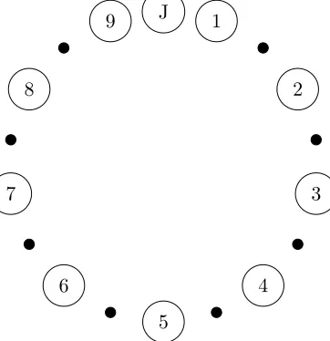
SOLUTION.Let’s begin by arbitrarily placing Joy somewhere at the table, and seating everyone else relative to her. This effectively distinguishes the other eleven seats. Next, we’ll consider the nine people who aren’t in Joy’s family, and place them (standing) in an order clockwise around the table from her. There are 33!/(33−9)! ways to do this. Before we actually assign seats to these nine people, we decide where to slot in Dave and Harmony amongst them.

J ₁

2

3

4

5 6

7 8

9

(In the above diagram, the digits 1 through 9 represent the nine other people who are sitting at the Morris family’s table, and the J represents Joy’s position.) Dave can sit between any pair of non-Morrises who are standing beside each other; that is, in any of the spots marked by small black dots in the diagram above. Thus, there are eight possible choices for where Dave will sit. Now Harmony can go into any of the remaining seven spots marked by black dots. Once Dave and Harmony are in place, everyone shifts to even out the circle (so the remaining black dots disappear), and takes their seats in the order determined.

We have shown that there are 33!/24!·8·7 possible seating arrangements at the Morris table. That’s a really big number, and it’s quite acceptable to leave it in this format. However, in case you find another way to work out the problem and want to check your answer, the total number is 783,732,837,888,000.

EXERCISES 3.8. Use what you have learned about permutations to work out the following problems. The sum and/or product rule may also be required.

1) Six people, all of whom can play both bass and guitar, are auditioning for a band. There are two spots available: lead guitar, and bass player. In how many ways can the band be completed?

2) Your friend Garth tries out for a play. After the auditions, he texts you that he got one of the parts he wanted, and that (including him) nine people tried out for the five roles. You know that there were two parts that interested him. In how many ways might the cast be completed (who gets which role matters)?

(27)

the password. You are not allowed to use any character more than once. How many different passwords can you create?

4) How many 3-letter “words” (strings of characters, they don’t actually have to be words) can you form from the letters of the word STRONG? How many of those words contain an s? (You may not use a letter more than once.)

5) How many permutations of{0,1,2,3,4,5,6}have no adjacent even digits? For example, a permutation like 5034216 is not allowed because 4 and 2 are adjacent.

3B. Combinations

Sometimes the order in which individuals are chosen doesn’t matter; all that matters is whether or not they were chosen. An example of this is choosing a set of problems for an exam. Although the order in which the questions are arranged may make the exam more or less intimidating, what really matters is which questions are on the exam, and which are not. Another example would be choosing shirts to pack for a trip (assuming all of your shirts are distinguishable from each other). We call a choice like this a “combination,” to indicate that it is the collection of things chosen that matters, and not the order.

DEFINITION 3.9.Let n be a positive natural number, and 0≤r ≤n. Assume that we have

ndistinct objects. Anr-combinationof thenobjects is a subset consisting ofr of the objects. So a combination involves choosing items from a finite population in which every item is uniquely identified, but the order in which the choices are made is unimportant.

Again, you should not be surprised to learn (since we are studying enumeration) that what we’ll be asking ishow many combinations there are, in a variety of circumstances. One signifi-cant difference from permutations is that it’s not interesting to ask how many n-combinations there are of nobjects; there is only one, as we must choose all of the objects.

Let’s begin with an example in which we’ll calculate the number of 3-combinations of ten objects (or in this case, people).

EXAMPLE 3.10.Of the ten athletes competing for Olympic medals in women’s speed skating (1000 metres), three are to be chosen to form a committee to review the rules for future competitions. How many different committees could be formed?

SOLUTION.We determined in Example 3.2 that there are 10!/7! ways in which the medals can be assigned. One easy way to choose the committee would be to make it consist of the three medal-winners. However, notice that if (for example) Wong wins gold, ˇSajna wins silver, and Andersen wins bronze, we will end up with the same committee as if ˇSajna wins gold, Andersen wins silver, and Wong wins bronze. In fact, what we’ve learned about permutations tells us that there are 3! different medal outcomes that would each result in the committee being formed of Wong, ˇSajna, and Andersen.

In fact, there’s nothing special about Wong, ˇSajna, and Andersen – for any choice of three people to be on the committee, there are 3! = 6 ways in which those individuals could have been awarded the medals. Therefore, when we counted the number of ways in which the medals could be assigned, we counted each possible 3-member committee exactly 3! = 6 times. So the number of different committees is 10!/(7!3!) = 10·9·8/6 = 120.

We can use the same reasoning to determine a general formula for the number of r -combinations ofn objects:

THEOREM 3.11.The number of r-combinations of n objects is

n!

(28)

PROOF.By Theorem 3.3, there are n!/(n−r)! r-permutations ofnobjects. Suppose that we knew there are k unordered r-subsets of n objects (i.e. r-combinations). For each of these k

unordered subsets, there are r! ways in which we could order the elements. This tells us that

k·r! =n!/(n−r)!. Rearranging the equation, we obtaink=n!/(r!(n−r)!).

It will also prove extremely useful to have a short form for the number of r-combinations of nobjects.

NOTATION 3.12.We use n_r

to denote the number ofr-combinations of nobjects, so

n r

= n!

r!(n−r)!.

DEFINITION 3.13.We read n_r as “n choose r,” son chooser isn!/[r!(n−r)!]. Notice that when r=n, we have

n r

= n!

n!(n−n)! =

n!

n!0! =

n!

n! = 1,

coinciding with our earlier observation that there is only one way in which all of thenobjects can be chosen. Similarly,

n

0

= n!

0!(n−0)! = 1; there is exactly one way of choosing none of the nobjects.

Let’s go over another example that involves combinations.

EXAMPLE 3.14.Jasmine is holding three cards from a regular deck of playing cards. She tells you that they are all hearts, and that she is holding at least one of the two highest cards in the suit (Ace and King). If you wanted to list all of the possible sets of cards she might be holding, how long would your list be?

SOLUTION.We’ll consider three cases: that Jasmine is holding the Ace (but not the King); that she is holding the King (but not the Ace), or that she is holding both the Ace and the King.

If Jasmine is holding the Ace but not the King, of the eleven other cards in the suit of hearts she must be holding two. There are 11₂

possible choices for the cards she is holding in this case.

Similarly, if Jasmine is holding the King but not the Ace, of the eleven other cards in the suit of hearts she must be holding two. Again, there are 11₂ possible choices for the cards she is holding in this case.

Finally, if Jasmine is holding the Ace and the King, then she is holding one of the other eleven cards in the suit of hearts. There are 11₁

possible choices for the cards she is holding in this case.

In total, you would have to list

11 2 + 11 2 + 11 1 = 11! 2!9! + 11! 2!9! + 11! 1!10! =

11·10

2 +

11·10

2 + 11 = 55 + 55 + 11 = 121 possible sets of cards.

(29)

A common mistake in an example like this, is to divide the problem into the cases that Jasmine is holding the Ace, or that she is holding the King, and to determine that each of these cases includes 12₂

= 66 possible combinations of cards, for a total of 132. The problem with this analysis is that we’ve counted the combinations that include both the Ace and the King twice: once as a combination that includes the Ace, and once as a combination that includes the King. If you do this, you need to compensate by subtracting at the end the number of combinations that have been counted twice: that is, those that include the Ace and the King. As we worked out in the example, there are 11₁= 11 of these, making a total of 132−11 = 121 combinations.

EXERCISES 3.15.Use what you have learned about combinations to work out the following problems. Permutations and other counting rules we’ve covered may also be required.

1) For a magic trick, you ask a friend to draw three cards from a standard deck of 52 cards. How many possible sets of cards might she have chosen?

2) For the same trick, you insist that your friend keep replacing her first draw until she draws a card that isn’t a spade. She can choose any cards for her other two cards. How many possible sets of cards might she end up with? (Caution: choosing 5♣,6♦,3♠in that order, is not different from choosing 6♦,5♣,3♠ in that order. You do not need to take into account that some sets will be more likely to occur than others.)

3) How many 5-digit numbers contain exactly two zeroes? (We insist that the number contain exactly 5 digits.)

4) Sandeep, Hee, Sara, and Mohammad play euchre with a standard deck consisting of 24 cards (A, K, Q, J, 10, and 9 from each of the four suits of a regular deck of playing cards). In how many ways can the deck be dealt so that each player receives 5 cards, with 4 cards left in the middle, one of which is turned face-up? The order of the 3 cards that are left face-down in the middle does not matter, but who receives a particular set of 5 cards (for example, Sara or Sandeep) does matter.

5) An ice cream shop has 10 flavours of ice cream and 7 toppings. Their megasundae consists of your choice of any 3 flavours of ice cream and any 4 toppings. (A customer must choose exactly three different flavours of ice cream and four different toppings.) How many different megasundaes are there?

3C. The Binomial Theorem

Here is an algebraic example in which “nchoose r” arises naturally.

EXAMPLE 3.16. Consider

(a+b)4 = (a+b)(a+b)(a+b)(a+b).

If you try to multiply this out, you must systematically choose the a or the b from each of the four factors, and make sure that you make every possible combination of choices sooner or later.

(30)

of a particular termaib4−i will be the number of ways in which you can chooseiof the factors from which to take an a, taking ab from the other 4−ifactors (where 0≤i≤4).

Let’s go through each of these cases separately. By Theorem 3.11, there is 4₄

= 1 way to choose four factors from which to take as. (Clearly, you must choose an a from every one of the four factors.) Thus, the coefficient of a4 will be 1.

If you want to take as from three of the four factors, Theorem 3.11 tells us that there are 4

3

= 4 ways in which to choose the factors from which you take the as. (Specifically, these four ways consist of taking the b from any one of the four factors, and the as from the other three factors). Thus, the coefficient ofa3bwill be 4.

If you want to takeas from two of the four factors, andbs from the other two, Theorem 3.11 tells us that there are 4₂= 6 ways in which to choose the factors from which you take the as (then takebs from the other two factors). This is a small enough example that you could easily work out all six ways by hand if you wish. Thus, the coefficient ofa2b2 will be 6.

If you want to take as from one of the four factors, Theorem 3.11 tells us that there are 4

1

= 4 ways in which to choose the factors from which you take the as. (Specifically, these four ways consist of taking the a from any one of the four factors, and the bs from the other three factors). Thus, the coefficient ofab3 will be 4.

Finally, by Theorem 3.11, there is 4₀

= 1 way to choose zero factors from which to take

as. (Clearly, you must choose a b from every one of the four factors.) Thus, the coefficient of

b4 will be 1.

Putting all of this together, we see that

(a+b)4 =a4+ 4a3b+ 6a2b2+ 4ab3+b4.

In fact, if we leave the coefficients in the original form in which we worked them out, we see that

(a+b)4=

4 4

a4+

4 3

a3b+

4 2

a2b2+

4 1

ab3+

4 0

b4.

This example generalises into a significant theorem of mathematics:

THEOREM 3.17. Binomial Theorem For any aand b, and any natural number n, we have

(a+b)n=

n X r=0 n r

arbn−r.

One special case of this is that

(1 +x)n=

n X r=0 n r

xr.

PROOF.As in Example 3.16, we see that the coefficient ofarbn−rin (a+b)nwill be the number of ways of choosingr of the nfactors from which we’ll take thea(taking theb from the other

n−r factors). By Theorem 3.11, there are n_r

ways of making this choice.

For the special case, begin by observing that (1 +x)n= (x+ 1)n; then takea=xandb= 1 in the general formula. Use the fact that 1n−r = 1 for any integersnand r.

Thus, the values n_r are the coefficients of the terms in the Binomial Theorem.

(31)

COROLLARY 3.19.For any natural numbern, we have

n

X

r=0

n r

= 2n.

PROOF.This is an immediate consequence of substituting a=b= 1 into the Binomial Theo-rem.

COROLLARY 3.20.For any natural numbern, we have

n

X

r=0

r

n r

(−1)r−1= 0.

PROOF.From the special case of the Binomial Theorem, we have

(1 +x)n=

n

X

r=0

n r

xr.

If we differentiate both sides, we obtain

n(1 +x)n−1 =

n

X

r=0

r

n r

xr−1.

Substituting x=−1 gives the result (the left-hand side is zero).

EXERCISES 3.21. Use the Binomial Theorem to evaluate the following: 1)Pn

i=1

n i

2i_.

(32)

SUMMARY:

•The number of r-permutations ofnobjects is n!/(n−r)!.

•The number of r-combinations of nobjects is n_r

= _r_!(_nn₋!_r_)!.

•The Binomial Theorem

•Important definitions:

◦permutation,r-permutation

◦nfactorial

◦r-combination

◦nchoose r

◦binomial coefficients

•Notation:

◦n!

(33)

Chapter 4

Bijections and

Combinatorial

Proofs

You may recall that in Math 2000 you learned that two sets have the same cardinality if there is a bijection between them. (A bijection is a one-to-one, onto function.) This leads us to another important method for counting a set: we come up with a bijection between the elements of the unknown set, and the elements of a set that we do know how to count. This idea is very closely related to the concept of a combinatorial proof, which we will explore in the second half of this chapter.

Aside: Although we won’t explore the concepts ofP andNP at all in this course, those of you who have studied these ideas in computer science courses may be interested to learn that most of the techniques used to prove that a particular problem is in P or in NP are related to the techniques discussed in this chapter. Usually a problem X is proven to be in NP (for example) by starting with a problem Y that is already known to be in NP. Then the scientist uses some clever ideas to show that problemY can be related to problemXin such a way that if problem X could be solved in polynomial time, that solution would produce a solution to problem Y, still in polynomial time. Thus the fact thatY is in NP forcesX to be inNP also. The same ideas may sometimes relate the number of solutions of problem X to the number of solutions of problem Y.

4A. Counting via bijections

It can be hard to figure out how to count the number of outcomes for a particular problem. Sometimes it will be possible to find a different problem, and to prove that the two problems have the same number of outcomes (by finding a bijection between their outcomes). If we can work out how to count the outcomes for the second problem, then we’ve also solved the first problem! This may seem blatantly obvious intuitively, but this technique can provide simple solutions to problems that at first glance seem very difficult.

This technique of counting a set (or the number of outcomes to some problem) indirectly, via a different set or problem, is the bijective technique for counting. We begin with a classic example of this technique.

EXAMPLE 4.1. How many possible subsets are there, from a set ofnelements?

SOLUTION.One approach would be to figure out how many 0-element subsets there are, how many 1-element subsets, etc., and add up all of the values we find. This works, but there are

(34)

so many pieces involved that it is prone to error. Also, the value will not be easy to calculate oncen gets reasonably large.

Instead, we imagine creating a table. The columns are indexed by the elements of the set, so there are n columns. We index the rows by the subsets of our set (one per row). In each entry of the table, we place a 1 if the subset that corresponds to this row contains the element that corresponds to this column. Here’s an example of such a table when the set is{x, y, z}:

x y z

∅ 0 0 0

{x} 1 0 0

{y} 0 1 0

{z} 0 0 1

{x, y} 1 1 0

{x, z} 1 0 1

{y, z} 0 1 1

{x, y, z} 1 1 1

As you can see, the pattern of 1s and 0s is different in each row of the table, since the elements of each subset are different. Furthermore, any pattern of 1s and 0s that has length 3, appears in some row of this table.

This is not a coincidence. In general, we can define a bijection between the binary strings of lengthn, and the subsets of a set ofnelements, as follows. We already know by the definition of cardinality, that there is a bijection between our set of n elements, and the set {1, . . . , n}, so we’ll actually define a bijection between the subsets of {1, . . . , n} and the binary strings of length n. Since the composition of two bijections is a bijection, this will indirectly define a bijection between

Combinatorics

Combinatorics

Contents

Part II.

Part III.

Chapter 1

SUMMARY:

Part I

EXERCISES 2.18.

SUMMARY:

Permutations,

SUMMARY:

Chapter 4