Calculus Volume 1
SENIOR CONTRIBUTING AUTHORS
E
DWIN
"J
ED
"
H
ERMAN
,
U
NIVERSITY OF
W
ISCONSIN
-S
TEVENS
P
OINT
G
ILBERT
S
TRANG
,
M
ASSACHUSETTS
I
NSTITUTE OF
T
ECHNOLOGY
Rice University
6100 Main Street MS-375 Houston, Texas 77005
To learn more about OpenStax, visit https://openstax.org.
Individual print copies and bulk orders can be purchased through our website.
©2018 Rice University. Textbook content produced by OpenStax is licensed under a Creative Commons Attribution Non-Commercial ShareAlike 4.0 International License (CC BY-NC-SA 4.0). Under this license, any user of this textbook or the textbook contents herein can share, remix, and build upon the content for noncommercial purposes only. Any adaptations must be shared under the same type of license. In any case of sharing the original or adapted material, whether in whole or in part, the user must provide proper attribution as follows:
- If you noncommercially redistribute this textbook in a digital format (including but not limited to PDF and HTML), then you must retain on every page the following attribution:
“Download for free at https://openstax.org/details/books/calculus-volume-1.”
- If you noncommercially redistribute this textbook in a print format, then you must include on every physical page the following attribution:
“Download for free at https://openstax.org/details/books/calculus-volume-1.”
- If you noncommercially redistribute part of this textbook, then you must retain in every digital format page view (including but not limited to PDF and HTML) and on every physical printed page the following attribution: “Download for free at https://openstax.org/details/books/calculus-volume-1.”
- If you use this textbook as a bibliographic reference, please include https://openstax.org/details/books/calculus-volume-1 in your citation.
For questions regarding this licensing, please contact [email protected].
Trademarks
The OpenStax name, OpenStax logo, OpenStax book covers, OpenStax CNX name, OpenStax CNX logo, OpenStax Tutor name, Openstax Tutor logo, Connexions name, Connexions logo, Rice University name, and Rice University logo are not subject to the license and may not be reproduced without the prior and express written consent of Rice University.
O
PENS
TAXOpenStax provides free, peer-reviewed, openly licensed textbooks for introductory college and Advanced Placement® courses and low-cost, personalized courseware that helps students learn. A nonprofit ed tech initiative based at Rice University, we’re committed to helping students
access the tools they need to complete their courses and meet their educational goals.
R
ICEU
NIVERSITYOpenStax, OpenStax CNX, and OpenStax Tutor are initiatives of Rice University. As a leading research university with a distinctive commitment to undergraduate education, Rice University aspires to path-breaking research, unsurpassed teaching, and contributions to the betterment of our world. It seeks to fulfill this mission by cultivating a diverse community of learning and discovery that produces leaders across the spectrum of human endeavor.
F
OUNDATIONS
UPPORTOpenStax is grateful for the tremendous support of our sponsors. Without their strong engagement, the goal of free access to high-quality textbooks would remain just a dream.
Laura and John Arnold Foundation (LJAF) actively seeks opportunities to invest in organizations and thought leaders that have a sincere interest in implementing fundamental changes that not only yield immediate gains, but also repair broken systems for future generations. LJAF currently focuses its strategic investments on education, criminal justice, research integrity, and public accountability.
The William and Flora Hewlett Foundation has been making grants since 1967 to help solve social and environmental problems at home and around the world. The Foundation concentrates its resources on activities in education, the environment, global development and population, performing arts, and philanthropy, and makes grants to support disadvantaged communities in the San Francisco Bay Area.
Calvin K. Kazanjian was the founder and president of Peter Paul (Almond Joy), Inc. He firmly believed that the more people understood about basic economics the happier and more prosperous they would be. Accordingly, he established the Calvin K. Kazanjian Economics Foundation Inc, in 1949 as a philanthropic, nonpolitical educational organization to support efforts that enhanced economic understanding.
Guided by the belief that every life has equal value, the Bill & Melinda Gates Foundation works to help all people lead healthy, productive lives. In developing countries, it focuses on improving people’s health with vaccines and other
life-saving tools and giving them the chance to lift themselves out of hunger and extreme poverty. In the United States, it seeks to significantly improve education so that all young people have the opportunity to reach their full potential. Based in Seattle, Washington, the foundation is led by CEO Jeff Raikes and Co-chair William H. Gates Sr., under the direction of Bill and Melinda Gates and Warren Buffett.
The Maxfield Foundation supports projects with potential for high impact in science, education, sustainability, and other areas of social importance.
Our mission at The Michelson 20MM Foundation is to grow access and success by eliminating unnecessary hurdles to affordability. We support the creation, sharing, and proliferation of more effective, more affordable educational content by leveraging disruptive technologies, open educational resources, and new models for collaboration between for-profit, nonprofit, and public entities.
Access. The future of education.
OpenStax.org
I like free textbooks
and I cannot lie.
to OpenStax and
we’ll send you a
sticker!
OpenStax is a nonprofit initiative, which means that that every dollar you give helps us maintain and grow our library of free textbooks.
Chapter 1: Functions and Graphs . . . 7
1.1 Review of Functions . . . 8
1.2 Basic Classes of Functions . . . 36
1.3 Trigonometric Functions . . . 62
1.4 Inverse Functions . . . 78
1.5 Exponential and Logarithmic Functions . . . 96
Chapter 2: Limits . . . 123
2.1 A Preview of Calculus . . . 124
2.2 The Limit of a Function . . . 135
2.3 The Limit Laws . . . 160
2.4 Continuity . . . 179
2.5 The Precise Definition of a Limit . . . 194
Chapter 3: Derivatives . . . 213
3.1 Defining the Derivative . . . 214
3.2 The Derivative as a Function . . . 232
3.3 Differentiation Rules . . . 247
3.4 Derivatives as Rates of Change . . . 266
3.5 Derivatives of Trigonometric Functions . . . 277
3.6 The Chain Rule . . . 287
3.7 Derivatives of Inverse Functions . . . 299
3.8 Implicit Differentiation . . . 309
3.9 Derivatives of Exponential and Logarithmic Functions . . . 319
Chapter 4: Applications of Derivatives . . . 341
4.1 Related Rates . . . 342
4.2 Linear Approximations and Differentials . . . 354
4.3 Maxima and Minima . . . 366
4.4 The Mean Value Theorem . . . 379
4.5 Derivatives and the Shape of a Graph . . . 390
4.6 Limits at Infinity and Asymptotes . . . 407
4.7 Applied Optimization Problems . . . 439
4.8 L’Hôpital’s Rule . . . 454
4.9 Newton’s Method . . . 472
4.10 Antiderivatives . . . 485
Chapter 5: Integration . . . 507
5.1 Approximating Areas . . . 508
5.2 The Definite Integral . . . 529
5.3 The Fundamental Theorem of Calculus . . . 549
5.4 Integration Formulas and the Net Change Theorem . . . 566
5.5 Substitution . . . 584
5.6 Integrals Involving Exponential and Logarithmic Functions . . . 595
5.7 Integrals Resulting in Inverse Trigonometric Functions . . . 608
Chapter 6: Applications of Integration . . . 623
6.1 Areas between Curves . . . 624
6.2 Determining Volumes by Slicing . . . 636
6.3 Volumes of Revolution: Cylindrical Shells . . . 656
6.4 Arc Length of a Curve and Surface Area . . . 671
6.5 Physical Applications . . . 685
6.6 Moments and Centers of Mass . . . 703
6.7 Integrals, Exponential Functions, and Logarithms . . . 721
6.8 Exponential Growth and Decay . . . 734
6.9 Calculus of the Hyperbolic Functions . . . 745
Appendix A: Table of Integrals . . . 763
Appendix B: Table of Derivatives . . . 769
Appendix C: Review of Pre-Calculus . . . 771
PREFACE
Welcome toCalculus Volume 1, an OpenStax resource. This textbook was written to increase student access to high-quality
learning materials, maintaining highest standards of academic rigor at little to no cost.
About OpenStax
OpenStax is a nonprofit based at Rice University, and it’s our mission to improve student access to education. Our first openly licensed college textbook was published in 2012, and our library has since scaled to over 25 books for college
and AP®courses used by hundreds of thousands of students. OpenStax Tutor, our low-cost personalized learning tool, is
being used in college courses throughout the country. Through our partnerships with philanthropic foundations and our alliance with other educational resource organizations, OpenStax is breaking down the most common barriers to learning and empowering students and instructors to succeed.
About OpenStax's resources
CustomizationCalculus Volume 1is licensed under a Creative Commons Attribution 4.0 International (CC BY) license, which means that you can distribute, remix, and build upon the content, as long as you provide attribution to OpenStax and its content contributors.
Because our books are openly licensed, you are free to use the entire book or pick and choose the sections that are most relevant to the needs of your course. Feel free to remix the content by assigning your students certain chapters and sections in your syllabus, in the order that you prefer. You can even provide a direct link in your syllabus to the sections in the web view of your book.
Instructors also have the option of creating a customized version of their OpenStax book. The custom version can be made available to students in low-cost print or digital form through their campus bookstore. Visit your book page on OpenStax.org for more information.
Errata
All OpenStax textbooks undergo a rigorous review process. However, like any professional-grade textbook, errors sometimes occur. Since our books are web based, we can make updates periodically when deemed pedagogically necessary. If you have a correction to suggest, submit it through the link on your book page on OpenStax.org. Subject matter experts review all errata suggestions. OpenStax is committed to remaining transparent about all updates, so you will also find a list of past errata changes on your book page on OpenStax.org.
Format
You can access this textbook for free in web view or PDF through OpenStax.org, and for a low cost in print.
About
Calculus Volume 1
Calculus is designed for the typical two- or three-semester general calculus course, incorporating innovative features to enhance student learning. The book guides students through the core concepts of calculus and helps them understand how those concepts apply to their lives and the world around them. Due to the comprehensive nature of the material, we are offering the book in three volumes for flexibility and efficiency. Volume 1 covers functions, limits, derivatives, and integration.
Coverage and scope
OurCalculus Volume 1textbook adheres to the scope and sequence of most general calculus courses nationwide. We have worked to make calculus interesting and accessible to students while maintaining the mathematical rigor inherent in the
subject. With this objective in mind, the content of the three volumes ofCalculushave been developed and arranged to
provide a logical progression from fundamental to more advanced concepts, building upon what students have already learned and emphasizing connections between topics and between theory and applications. The goal of each section is to enable students not just to recognize concepts, but work with them in ways that will be useful in later courses and future careers. The organization and pedagogical features were developed and vetted with feedback from mathematics educators dedicated to the project.
Chapter 1: Functions and Graphs Chapter 2: Limits
Chapter 3: Derivatives
Chapter 4: Applications of Derivatives Chapter 5: Integration
Chapter 6: Applications of Integration
Volume 2
Chapter 1: Integration
Chapter 2: Applications of Integration Chapter 3: Techniques of Integration
Chapter 4: Introduction to Differential Equations Chapter 5: Sequences and Series
Chapter 6: Power Series
Chapter 7: Parametric Equations and Polar Coordinates
Volume 3
Chapter 1: Parametric Equations and Polar Coordinates Chapter 2: Vectors in Space
Chapter 3: Vector-Valued Functions
Chapter 4: Differentiation of Functions of Several Variables Chapter 5: Multiple Integration
Chapter 6: Vector Calculus
Chapter 7: Second-Order Differential Equations
Pedagogical foundation
ThroughoutCalculus Volume 1you will find examples and exercises that present classical ideas and techniques as well as
modern applications and methods. Derivations and explanations are based on years of classroom experience on the part of long-time calculus professors, striving for a balance of clarity and rigor that has proven successful with their students. Motivational applications cover important topics in probability, biology, ecology, business, and economics, as well as areas
of physics, chemistry, engineering, and computer science.Student Projectsin each chapter give students opportunities to
explore interesting sidelights in pure and applied mathematics, from determining a safe distance between the grandstand and the track at a Formula One racetrack, to calculating the center of mass of the Grand Canyon Skywalk or the terminal speed
of a skydiver.Chapter Opening Applicationspose problems that are solved later in the chapter, using the ideas covered in
that chapter. Problems include the hydraulic force against the Hoover Dam, and the comparison of relative intensity of two
earthquakes.Definitions, Rules,andTheoremsare highlighted throughout the text, including over 60Proofsof theorems.
Assessments that reinforce key concepts
In-chapterExampleswalk students through problems by posing a question, stepping out a solution, and then asking students
to practice the skill with a “Checkpoint” question. The book also includes assessments at the end of each chapter so
students can apply what they’ve learned through practice problems. Many exercises are marked with a[T]to indicate they
are suitable for solution by technology, including calculators or Computer Algebra Systems (CAS). Answers for selected
exercises are available in theAnswer Keyat the back of the book. The book also includes assessments at the end of each
chapter so students can apply what they’ve learned through practice problems.
Early or late transcendentals
Calculus Volume 1is designed to accommodate both Early and Late Transcendental approaches to calculus. Exponential and logarithmic functions are introduced informally in Chapter 1 and presented in more rigorous terms in Chapter 6. Differentiation and integration of these functions is covered in Chapters 3–5 for instructors who want to include them with other types of functions. These discussions, however, are in separate sections that can be skipped for instructors who prefer to wait until the integral definitions are given before teaching the calculus derivations of exponentials and logarithms.
diagrams, and photographs.
Additional resources
Student and instructor resourcesWe’ve compiled additional resources for both students and instructors, including Getting Started Guides, an instructor solution manual, and PowerPoint slides. Instructor resources require a verified instructor account, which can be requested on your OpenStax.org log-in. Take advantage of these resources to supplement your OpenStax book.
Community Hubs
OpenStax partners with the Institute for the Study of Knowledge Management in Education (ISKME) to offer Community Hubs on OER Commons – a platform for instructors to share community-created resources that support OpenStax books, free of charge. Through our Community Hubs, instructors can upload their own materials or download resources to use in their own courses, including additional ancillaries, teaching material, multimedia, and relevant course content. We encourage instructors to join the hubs for the subjects most relevant to your teaching and research as an opportunity both to enrich your courses and to engage with other faculty.
?To reach the Community Hubs, visitwww.oercommons.org/hubs/OpenStax.
Partner resources
OpenStax Partners are our allies in the mission to make high-quality learning materials affordable and accessible to students and instructors everywhere. Their tools integrate seamlessly with our OpenStax titles at a low cost. To access the partner resources for your text, visit your book page on OpenStax.org.
About the authors
Senior contributing authorsDr. Strang received his PhD from UCLA in 1959 and has been teaching mathematics at MIT ever since. His Calculus online textbook is one of eleven that he has published and is the basis from which our final product has been derived and updated for today’s student. Strang is a decorated mathematician and past Rhodes Scholar at Oxford University.
Edwin “Jed” Herman, University of Wisconsin-Stevens Point
Dr. Herman earned a BS in Mathematics from Harvey Mudd College in 1985, an MA in Mathematics from UCLA in 1987, and a PhD in Mathematics from the University of Oregon in 1997. He is currently a Professor at the University of Wisconsin-Stevens Point. He has more than 20 years of experience teaching college mathematics, is a student research mentor, is experienced in course development/design, and is also an avid board game designer and player.
Contributing authors
Catherine Abbott, Keuka College
Nicoleta Virginia Bila, Fayetteville State University Sheri J. Boyd, Rollins College
Joyati Debnath, Winona State University Valeree Falduto, Palm Beach State College Joseph Lakey, New Mexico State University Julie Levandosky, Framingham State University David McCune, William Jewell College Michelle Merriweather, Bronxville High School Kirsten R. Messer, Colorado State University - Pueblo Alfred K. Mulzet, Florida State College at Jacksonville
William Radulovich (retired), Florida State College at Jacksonville Erica M. Rutter, Arizona State University
David Smith, University of the Virgin Islands Elaine A. Terry, Saint Joseph’s University David Torain, Hampton University
Reviewers
Marwan A. Abu-Sawwa, Florida State College at Jacksonville Kenneth J. Bernard, Virginia State University
John Beyers, University of Maryland
Charles Buehrle, Franklin & Marshall College Matthew Cathey, Wofford College
Michael Cohen, Hofstra University
William DeSalazar, Broward County School System Murray Eisenberg, University of Massachusetts Amherst Kristyanna Erickson, Cecil College
Tiernan Fogarty, Oregon Institute of Technology David French, Tidewater Community College Marilyn Gloyer, Virginia Commonwealth University Shawna Haider, Salt Lake Community College Lance Hemlow, Raritan Valley Community College Jerry Jared, The Blue Ridge School
Peter Jipsen, Chapman University David Johnson, Lehigh University M.R. Khadivi, Jackson State University Robert J. Krueger, Concordia University Tor A. Kwembe, Jackson State University
Jean-Marie Magnier, Springfield Technical Community College Cheryl Chute Miller, SUNY Potsdam
Bagisa Mukherjee, Penn State University, Worthington Scranton Campus Kasso Okoudjou, University of Maryland College Park
Peter Olszewski, Penn State Erie, The Behrend College Steven Purtee, Valencia College
Alice Ramos, Bethel College
1
|
FUNCTIONS AND
GRAPHS
Figure 1.1 A portion of the San Andreas Fault in California. Major faults like this are the sites of most of the strongest earthquakes ever recorded. (credit: modification of work by Robb Hannawacker, NPS)
Chapter Outline
1.1Review of Functions 1.2Basic Classes of Functions 1.3Trigonometric Functions 1.4Inverse Functions
1.5Exponential and Logarithmic Functions
Introduction
In the past few years, major earthquakes have occurred in several countries around the world. In January 2010, an earthquake of magnitude 7.3 hit Haiti. A magnitude 9 earthquake shook northeastern Japan in March 2011. In April 2014, an 8.2-magnitude earthquake struck off the coast of northern Chile. What do these numbers mean? In particular, how does a magnitude 9 earthquake compare with an earthquake of magnitude 8.2? Or 7.3? Later in this chapter, we show how logarithmic functions are used to compare the relative intensity of two earthquakes based on the magnitude of each
earthquake (seeExample 1.39).
1.1
|
Review of Functions
Learning Objectives
1.1.1 Use functional notation to evaluate a function. 1.1.2 Determine the domain and range of a function. 1.1.3 Draw the graph of a function.
1.1.4 Find the zeros of a function.
1.1.5 Recognize a function from a table of values.
1.1.6 Make new functions from two or more given functions. 1.1.7 Describe the symmetry properties of a function.
In this section, we provide a formal definition of a function and examine several ways in which functions are represented—namely, through tables, formulas, and graphs. We study formal notation and terms related to functions. We also define composition of functions and symmetry properties. Most of this material will be a review for you, but it serves as a handy reference to remind you of some of the algebraic techniques useful for working with functions.
Functions
Given two sets A and B, a set with elements that are ordered pairs (x, y), where x is an element of A and y is an
element of B, is a relation from A to B. A relation from A to B defines a relationship between those two sets. A
function is a special type of relation in which each element of the first set is related to exactly one element of the second
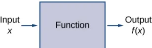
set. The element of the first set is called theinput; the element of the second set is called theoutput. Functions are used all
the time in mathematics to describe relationships between two sets. For any function, when we know the input, the output is determined, so we say that the output is a function of the input. For example, the area of a square is determined by its side length, so we say that the area (the output) is a function of its side length (the input). The velocity of a ball thrown in the air can be described as a function of the amount of time the ball is in the air. The cost of mailing a package is a function of the weight of the package. Since functions have so many uses, it is important to have precise definitions and terminology to study them.
Definition
Afunction f consists of a set of inputs, a set of outputs, and a rule for assigning each input to exactly one output. The
set of inputs is called thedomainof the function. The set of outputs is called therangeof the function.
For example, consider the function f , where the domain is the set of all real numbers and the rule is to square the input.
Then, the input x = 3 is assigned to the output 32= 9. Since every nonnegative real number has a real-value square root,
every nonnegative number is an element of the range of this function. Since there is no real number with a square that is negative, the negative real numbers are not elements of the range. We conclude that the range is the set of nonnegative real numbers.
For a general function f with domain D, we often use x to denote the input and y to denote the output associated with
x. When doing so, we refer to x as theindependent variableand y as thedependent variable, because it depends on x.
Using function notation, we write y = f (x), and we read this equation as “y equals f of x.” For the squaring function
described earlier, we write f (x) = x2.
Figure 1.2 A function can be visualized as an input/output device.
Figure 1.3 A function maps every element in the domain to exactly one element in the range. Although each input can be sent to only one output, two different inputs can be sent to the same output.
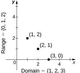
Figure 1.4 In this case, a graph of a function f has a domain of {1, 2, 3} and a range of {1, 2}. The independent variable is x and the dependent variable is y.
Visit this applet link (http://www.openstaxcollege.org/l/grapherrors) to see more about graphs of
functions.
We can also visualize a function by plotting points (x, y) in the coordinate plane where y = f (x). Thegraph of a function
is the set of all these points. For example, consider the function f , where the domain is the set D = {1, 2, 3} and the
[image:17.612.228.387.298.419.2]Figure 1.5 Here we see a graph of the function f with domain {1, 2, 3} and rule f (x) = 3 − x. The graph consists of the points (x, f (x)) for all x in the domain.
Every function has a domain. However, sometimes a function is described by an equation, as in f (x) = x2, with no
specific domain given. In this case, the domain is taken to be the set of all real numbers x for which f (x) is a real number.
For example, since any real number can be squared, if no other domain is specified, we consider the domain of f (x) = x2
to be the set of all real numbers. On the other hand, the square root function f (x) = x only gives a real output if x is
nonnegative. Therefore, the domain of the function f(x) = x is the set of nonnegative real numbers, sometimes called the
natural domain.
For the functions f (x) = x2 and f (x) = x, the domains are sets with an infinite number of elements. Clearly we cannot
list all these elements. When describing a set with an infinite number of elements, it is often helpful to use set-builder or
interval notation. When using set-builder notation to describe a subset of all real numbers, denoted ℝ, we write
⎧ ⎩
⎨x
|
x has some property⎫ ⎭ ⎬.We read this as the set of real numbers x such that x has some property. For example, if we were interested in the set of
real numbers that are greater than one but less than five, we could denote this set using set-builder notation by writing
{x
|
1 < x < 5}.A set such as this, which contains all numbers greater than a and less than b, can also be denoted using the interval
notation (a, b). Therefore,
(1, 5) =⎧ ⎩
⎨x
|
1 < x < 5⎫ ⎭ ⎬.The numbers 1 and 5 are called theendpointsof this set. If we want to consider the set that includes the endpoints, we
would denote this set by writing
[1, 5] = {x
|
1 ≤ x ≤ 5}.We can use similar notation if we want to include one of the endpoints, but not the other. To denote the set of nonnegative real numbers, we would use the set-builder notation
{x
|
0 ≤ x}.The smallest number in this set is zero, but this set does not have a largest number. Using interval notation, we would use
the symbol ∞, which refers to positive infinity, and we would write the set as
[0, ∞) = {x
|
0 ≤ x}.It is important to note that ∞ is not a real number. It is used symbolically here to indicate that this set includes all real
numbers greater than or equal to zero. Similarly, if we wanted to describe the set of all nonpositive numbers, we could write
1.1
Here, the notation −∞ refers to negative infinity, and it indicates that we are including all numbers less than or equal to
zero, no matter how small. The set
(−∞, ∞) =⎧ ⎩
⎨x
|
x is any real number⎫⎭⎬refers to the set of all real numbers.
Some functions are defined using different equations for different parts of their domain. These types of functions are known aspiecewise-defined functions. For example, suppose we want to define a function f with a domain that is the set of all
real numbers such that f (x) = 3x + 1 for x ≥ 2 and f (x) = x2 for x < 2. We denote this function by writing
f (x) =⎧⎩⎨3x + 1 x ≥ 2
x2 x < 2.
When evaluating this function for an input x, the equation to use depends on whether x ≥ 2 or x < 2. For example,
since 5 > 2, we use the fact that f (x) = 3x + 1 for x ≥ 2 and see that f (5) = 3(5) + 1 = 16. On the other hand, for
x = −1, we use the fact that f (x) = x2 for x < 2 and see that f (−1) = 1.
Example 1.1
Evaluating Functions
For the function f(x) = 3x2+ 2x − 1, evaluate
a. f(−2)
b. f( 2)
c. f (a + h)
Solution
Substitute the given value forxin the formula for f (x).
a. f(−2) = 3(−2)2+ 2(−2) − 1 = 12 − 4 − 1 = 7
b. f( 2) = 3( 2)2+ 2 2 − 1 = 6 + 2 2 − 1 = 5 + 2 2
c. f(a + h) = 3(a + h)2+ 2(a + h) − 1 = 3
⎛
⎝a2+ 2ah + h2⎞⎠+ 2a + 2h − 1
= 3a2+ 6ah + 3h2+ 2a + 2h − 1
For f (x) = x2− 3x + 5, evaluate f (1) and f (a + h).
Example 1.2
Finding Domain and Range
a. f (x) = (x − 4)2+ 5 b. f (x) = 3x + 2 − 1
c. f (x) = 3
x − 2
Solution
a. Consider f(x) = (x − 4)2+ 5.
i. Since f (x) = (x − 4)2+ 5 is a real number for any real number x, the domain of f is the
interval (−∞, ∞).
ii. Since (x − 4)2≥ 0, we know f(x) = (x − 4)2+ 5 ≥ 5. Therefore, the range must be a subset
of ⎧
⎩ ⎨y
|
y ≥ 5⎫⎭
⎬. To show that every element in this set is in the range, we need to show that for a
given y in that set, there is a real number x such that f (x) = (x − 4)2+ 5 = y. Solving this
equation for x, we see that we need x such that
(x − 4)2= y − 5.
This equation is satisfied as long as there exists a real number x such that
x − 4 = ± y − 5.
Since y ≥ 5, the square root is well-defined. We conclude that for x = 4 ± y − 5, f (x) = y,
and therefore the range is ⎧
⎩ ⎨y
|
y ≥ 5⎫⎭ ⎬.
b. Consider f(x) = 3x + 2 − 1.
i. To find the domain of f , we need the expression 3x + 2 ≥ 0. Solving this inequality, we
conclude that the domain is {x
|
x ≥ −2/3}.ii. To find the range of f , we note that since 3x + 2 ≥ 0, f (x) = 3x + 2 − 1 ≥ −1. Therefore,
the range of f must be a subset of the set ⎧
⎩
⎨y
|
y ≥ −1⎫ ⎭⎬. To show that every element in this set is
in the range of f , we need to show that for all y in this set, there exists a real number x in the
domain such that f (x) = y. Let y ≥ −1. Then, f (x) = y if and only if
3x + 2 − 1 = y.
Solving this equation for x, we see that x must solve the equation
3x + 2 = y + 1.
Since y ≥ −1, such an x could exist. Squaring both sides of this equation, we have
3x + 2 = (y + 1)2.
Therefore, we need
1.2
which implies
x = 13⎛
⎝y + 1⎞⎠2− 23.
We just need to verify that x is in the domain of f . Since the domain of f consists of all real
numbers greater than or equal to −2/3, and
1
3⎛⎝y + 1⎞⎠2− 23 ≥ − 23,
there does exist an x in the domain of f . We conclude that the range of f is ⎧
⎩
⎨y
|
y ≥ −1⎫ ⎭ ⎬.c. Consider f(x) = 3/(x − 2).
i. Since 3/(x − 2) is defined when the denominator is nonzero, the domain is {x
|
x ≠ 2}.ii. To find the range of f , we need to find the values of y such that there exists a real number x
in the domain with the property that
3
x − 2 = y.
Solving this equation for x, we find that
x = 3y + 2.
Therefore, as long as y ≠ 0, there exists a real number x in the domain such that f (x) = y.
Thus, the range is ⎧
⎩ ⎨y
|
y ≠ 0⎫⎭ ⎬.
Find the domain and range for f(x) = 4 − 2x + 5.
Representing Functions
Typically, a function is represented using one or more of the following tools:
• A table
• A graph
• A formula
We can identify a function in each form, but we can also use them together. For instance, we can plot on a graph the values from a table or create a table from a formula.
Tables
Functions described using atable of values arise frequently in real-world applications. Consider the following simple
example. We can describe temperature on a given day as a function of time of day. Suppose we record the temperature every
hour for a 24-hour period starting at midnight. We let our input variable x be the time after midnight, measured in hours,
and the output variable y be the temperature x hours after midnight, measured in degrees Fahrenheit. We record our data
Hours after Midnight Temperature (°F) Hours after Midnight Temperature (°F)
0 58 12 84
1 54 13 85
2 53 14 85
3 52 15 83
4 52 16 82
5 55 17 80
6 60 18 77
7 64 19 74
8 72 20 69
9 75 21 65
10 78 22 60
11 80 23 58
Table 1.1Temperature as a Function of Time of Day
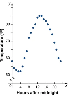
We can see from the table that temperature is a function of time, and the temperature decreases, then increases, and then decreases again. However, we cannot get a clear picture of the behavior of the function without graphing it.
Graphs
Given a function f described by a table, we can provide a visual picture of the function in the form of a graph. Graphing
the temperatures listed inTable 1.1can give us a better idea of their fluctuation throughout the day.Figure 1.6shows the
Figure 1.6 The graph of the data fromTable 1.1shows temperature as a function of time.
From the points plotted on the graph inFigure 1.6, we can visualize the general shape of the graph. It is often useful
to connect the dots in the graph, which represent the data from the table. In this example, although we cannot make any definitive conclusion regarding what the temperature was at any time for which the temperature was not recorded, given the number of data points collected and the pattern in these points, it is reasonable to suspect that the temperatures at other
times followed a similar pattern, as we can see inFigure 1.7.
Figure 1.7 Connecting the dots inFigure 1.6shows the general pattern of the data.
Algebraic Formulas
Sometimes we are not given the values of a function in table form, rather we are given the values in an explicit formula.
Formulas arise in many applications. For example, the area of a circle of radius r is given by the formula A(r) = πr2.
When an object is thrown upward from the ground with an initial velocity v0 ft/s, its height above the ground from the
time it is thrown until it hits the ground is given by the formula s(t) = −16t2+ v0t. When P dollars are invested in an
account at an annual interest rate r compounded continuously, the amount of money after t years is given by the formula
[image:23.612.235.380.366.567.2]Given an algebraic formula for a function f , the graph of f is the set of points ⎝x, f (x)⎠, where x is in the domain of
f and f (x) is in the range. To graph a function given by a formula, it is helpful to begin by using the formula to create
a table of inputs and outputs. If the domain of f consists of an infinite number of values, we cannot list all of them, but
because listing some of the inputs and outputs can be very useful, it is often a good way to begin.
When creating a table of inputs and outputs, we typically check to determine whether zero is an output. Those values of
x where f(x) = 0 are called thezeros of a function. For example, the zeros of f(x) = x2− 4 are x = ± 2. The zeros
determine where the graph of f intersects the x-axis, which gives us more information about the shape of the graph of
the function. The graph of a function may never intersect thex-axis, or it may intersect multiple (or even infinitely many)
times.
Another point of interest is the y-intercept, if it exists. The y-intercept is given by ⎛
⎝0, f (0)⎞⎠.
Since a function has exactly one output for each input, the graph of a function can have, at most, one y-intercept. If x = 0
is in the domain of a function f , then f has exactly one y-intercept. If x = 0 is not in the domain of f , then f has
no y-intercept. Similarly, for any real number c, if c is in the domain of f , there is exactly one output f(c), and the
line x = c intersects the graph of f exactly once. On the other hand, if c is not in the domain of f , f (c) is not defined
and the line x = c does not intersect the graph of f . This property is summarized in thevertical line test.
Rule: Vertical Line Test
Given a function f , every vertical line that may be drawn intersects the graph of f no more than once. If any vertical
line intersects a set of points more than once, the set of points does not represent a function.
We can use this test to determine whether a set of plotted points represents the graph of a function (Figure 1.8).
Figure 1.8 (a) The set of plotted points represents the graph of a function because every vertical line intersects the set of points, at most, once. (b) The set of plotted points does not represent the graph of a function because some vertical lines intersect the set of points more than once.
Finding Zeros and
y-Intercepts of a Function
Consider the function f(x) = −4x + 2.
a. Find all zeros of f .
b. Find the y-intercept (if any).
c. Sketch a graph of f .
Solution
a. To find the zeros, solve f (x) = −4x + 2 = 0. We discover that f has one zero at x = 1/2.
b. The y-intercept is given by ⎛
⎝0, f (0)⎞⎠= (0, 2).
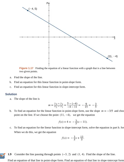
c. Given that f is a linear function of the form f(x) = mx + b that passes through the points (1/2, 0) and
(0, 2), we can sketch the graph of f (Figure 1.9).
Figure 1.9 The function f (x) = −4x + 2 is a line with x-intercept (1/2, 0) and y-intercept (0, 2).
Example 1.4
Using Zeros and
y-Intercepts to Sketch a Graph
Consider the function f (x) = x + 3 + 1.
a. Find all zeros of f .
b. Find the y-intercept (if any).
c. Sketch a graph of f .
Solution
1.3
x, this equation has no solutions, and therefore f has no zeros.
b. The y-intercept is given by ⎛
⎝0, f (0)⎞⎠= (0, 3 + 1).
c. To graph this function, we make a table of values. Since we need x + 3 ≥ 0, we need to choose values
of x ≥ −3. We choose values that make the square-root function easy to evaluate.
x −3 −2 1
f(x) 1 2 3
Table 1.2
Making use of the table and knowing that, since the function is a square root, the graph of f should be similar to
the graph of y = x, we sketch the graph (Figure 1.10).
Figure 1.10 The graph of f (x) = x + 3 + 1 has a y-intercept but no x-intercepts.
Find the zeros of f(x) = x3− 5x2+ 6x.
Example 1.5
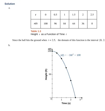
Finding the Height of a Free-Falling Object
If a ball is dropped from a height of 100ft, its height s at time t is given by the function s(t) = −16t2+ 100,
where s is measured in feet and t is measured in seconds. The domain is restricted to the interval [0, c], where
t = 0 is the time when the ball is dropped and t = c is the time when the ball hits the ground.
a. Create a table showing the height s(t) when t = 0, 0.5, 1, 1.5, 2, and 2.5. Using the data from the
table, determine the domain for this function. That is, find the time c when the ball hits the ground.
Solution a.
t 0 0.5 1 1.5 2 2.5
[image:27.612.74.481.67.497.2]s(t) 100 96 84 64 36 0
Table 1.3
Height s as a Function of Time t
Since the ball hits the ground when t = 2.5, the domain of this function is the interval [0, 2.5].
b.
Note that for this function and the function f(x) = −4x + 2 graphed in Figure 1.9, the values of f (x) are getting
smaller as x is getting larger. A function with this property is said to be decreasing. On the other hand, for the function
f(x) = x + 3 + 1 graphed inFigure 1.10, the values of f (x) are getting larger as the values of x are getting larger. A function with this property is said to be increasing. It is important to note, however, that a function can be increasing on some interval or intervals and decreasing over a different interval or intervals. For example, using our temperature function inFigure 1.6, we can see that the function is decreasing on the interval (0, 4), increasing on the interval (4, 14), and
then decreasing on the interval (14, 23). We make the idea of a function increasing or decreasing over a particular interval
more precise in the next definition.
Definition
We say that a function f isincreasing on the interval I if for all x1, x2∈ I,
f (x1) ≤ f (x2) when x1< x2.
f (x1) < f (x2) when x1< x2.
We say that a function f isdecreasing on the interval I if for all x1, x2∈ I,
f (x1) ≥ f (x2) if x1< x2.
We say that a function f is strictly decreasing on the interval I if for all x1, x2∈ I,
f (x1) > f (x2) if x1< x2.
For example, the function f (x) = 3x is increasing on the interval (−∞, ∞) because 3x1< 3x2 whenever x1< x2.
On the other hand, the function f(x) = −x3 is decreasing on the interval (−∞, ∞) because −x13> − x23 whenever
[image:28.612.127.478.232.550.2]x1< x2 (Figure 1.11).
Figure 1.11 (a) The function f (x) = 3x is increasing on the interval (−∞, ∞). (b) The function f(x) = −x3 is decreasing on the interval (−∞, ∞).
Combining Functions
Now that we have reviewed the basic characteristics of functions, we can see what happens to these properties when we combine functions in different ways, using basic mathematical operations to create new functions. For example, if the cost
for a company to manufacture x items is described by the function C(x) and the revenue created by the sale of x items is
described by the function R(x), then the profit on the manufacture and sale of x items is defined as P(x) = R(x) − C(x).
Using the difference between two functions, we created a new function.
Alternatively, we can create a new function by composing two functions. For example, given the functions f(x) = x2 and
g(x) = 3x + 1, the composite function f ∘g is defined such that
⎛
1.4
The composite function g∘ f is defined such that
⎛
⎝g∘ f⎞⎠(x) = g⎛⎝f(x)⎞⎠= 3 f (x) + 1 = 3x2+ 1.
Note that these two new functions are different from each other.
Combining Functions with Mathematical Operators
To combine functions using mathematical operators, we simply write the functions with the operator and simplify. Given
two functions f and g, we can define four new functions:
⎛
⎝f + g⎞⎠(x) = f (x) + g(x) Sum ⎛
⎝f − g⎞⎠(x) = f (x) − g(x) Diffe ence ⎛
⎝f · g⎞⎠(x) = f (x)g(x) Product
⎛
⎝gf⎞⎠(x) = f (x)g(x) for g(x) ≠ 0 Quotient
Example 1.6
Combining Functions Using Mathematical Operations
Given the functions f(x) = 2x − 3 and g(x) = x2− 1, find each of the following functions and state its
domain.
a. ( f + g)(x) b. ( f − g)(x) c. ( f · g)(x)
d. ⎛⎝gf⎞⎠(x)
Solution
a. ⎛
⎝f + g⎞⎠(x) = (2x − 3) + (x2− 1) = x2+ 2x − 4. The domain of this function is the interval (−∞, ∞).
b. ⎛
⎝f − g⎞⎠(x) = (2x − 3) − (x2− 1) = −x2+ 2x − 2. The domain of this function is the interval
(−∞, ∞).
c. ⎛
⎝f · g⎞⎠(x) = (2x − 3)(x2− 1) = 2x3− 3x2− 2x + 3. The domain of this function is the interval
(−∞, ∞).
d. ⎛⎝gf⎞⎠(x) = 2x − 3
x2− 1. The domain of this function is {x
|
x ≠ ±1}.For f(x) = x2+ 3 and g(x) = 2x − 5, find ⎛
⎝f /g⎞⎠(x) and state its domain.
Function Composition
When we compose functions, we take a function of a function. For example, suppose the temperature T on a given day is
described as a function of time t (measured in hours after midnight) as inTable 1.1. Suppose the cost C, to heat or cool
the cost of heating or cooling a building as a function of time by evaluating C⎝T(t)⎠. We have defined a new function,
denoted C∘T, which is defined such that (C∘T)(t) = C(T(t)) for all t in the domain of T. This new function is called
a composite function. We note that since cost is a function of temperature and temperature is a function of time, it makes
sense to define this new function (C∘T)(t). It does not make sense to consider (T ∘C)(t), because temperature is not a
function of cost.
Definition
Consider the function f with domain A and range B, and the function g with domain D and range E. If B is a
subset of D, then thecomposite function (g∘ f )(x) is the function with domain A such that
(1.1)
⎛
⎝g∘ f⎞⎠(x) = g⎛⎝f(x)⎞⎠.
A composite function g∘ f can be viewed in two steps. First, the function f maps each input x in the domain of f to
its output f (x) in the range of f . Second, since the range of f is a subset of the domain of g, the output f (x) is an
element in the domain of g, and therefore it is mapped to an output g⎛
⎝f(x)⎞⎠ in the range of g. InFigure 1.12, we see a
visual image of a composite function.
Figure 1.12 For the composite function g∘ f , we have ⎛
⎝g∘ f⎞⎠(1) = 4,⎛⎝g∘ f⎠⎞(2) = 5, and ⎛⎝g∘ f⎞⎠(3) = 4.
Example 1.7
Compositions of Functions Defined by Formulas
Consider the functions f (x) = x2+ 1 and g(x) = 1/x.
a. Find (g∘ f )(x) and state its domain and range.
b. Evaluate (g∘ f )(4), (g∘ f )(−1/2).
c. Find ( f ∘g)(x) and state its domain and range.
d. Evaluate ( f ∘g)(4), ( f ∘g)(−1/2).
Solution
a. We can find the formula for (g∘ f )(x) in two different ways. We could write
(g∘ f )(x) = g( f (x)) = g(x2+ 1) = 1
Alternatively, we could write
(g∘ f )(x) = g⎛
⎝f (x)⎞⎠= 1f (x) = 1
x2+ 1.
Since x2+ 1 ≠ 0 for all real numbers x, the domain of (g∘ f )(x) is the set of all real numbers. Since
0 < 1/(x2+ 1) ≤ 1, the range is, at most, the interval (0, 1]. To show that the range is this entire
interval, we let y = 1/(x2+ 1) and solve this equation for x to show that for all y in the interval
(0, 1], there exists a real number x such that y = 1/(x2+ 1). Solving this equation for x, we see that x2+ 1 = 1/y, which implies that
x = ± 1y − 1.
If y is in the interval (0, 1], the expression under the radical is nonnegative, and therefore there exists
a real number x such that 1/(x2+ 1) = y. We conclude that the range of g∘ f is the interval (0, 1].
b. (g∘ f )(4) = g( f (4)) = g(42+ 1) = g(17) = 1
17 (g∘ f )⎛⎝−12⎞⎠= g⎛⎝f⎛⎝−12⎞⎠⎞⎠= g⎛
⎝ ⎜⎛⎝−12⎞⎠
2
+ 1⎞
⎠
⎟= g⎛⎝54⎞⎠= 45
c. We can find a formula for ( f ∘g)(x) in two ways. First, we could write
( f ∘g)(x) = f (g(x)) = f⎛⎝1x⎞⎠=⎛⎝1x⎞⎠2+ 1.
Alternatively, we could write
( f ∘g)(x) = f (g(x)) = (g(x))2+ 1 =⎛⎝1x⎞⎠2+ 1.
The domain of f ∘g is the set of all real numbers x such that x ≠ 0. To find the range of f , we need
to find all values y for which there exists a real number x ≠ 0 such that
⎛ ⎝1x⎞⎠
2
+ 1 = y.
Solving this equation for x, we see that we need x to satisfy
⎛ ⎝1x⎞⎠
2
= y − 1,
which simplifies to
1x = ± y − 1.
1.5
x = ± 1y − 1.
Since 1/ y − 1 is a real number if and only if y > 1, the range of f is the set ⎧
⎩ ⎨y
|
y ≥ 1⎫⎭ ⎬.
d. ( f ∘g)(4) = f (g(4)) = f⎛⎝14⎞⎠=⎛⎝14⎞⎠2+ 1 = 17
16 ( f ∘g)⎛⎝−12⎞⎠= f⎛⎝g⎛⎝−12⎞⎠⎞⎠= f (−2) = (−2)2+ 1 = 5
InExample 1.7, we can see that ⎛
⎝f ∘g⎞⎠(x) ≠⎛⎝g∘ f⎞⎠(x). This tells us, in general terms, that the order in which we compose
functions matters.
Let f(x) = 2 − 5x. Let g(x) = x. Find ⎛ ⎝f ∘g⎞⎠(x).
Example 1.8
Composition of Functions Defined by Tables
Consider the functions f and g described byTable 1.4andTable 1.5.
x −3 −2 −1 0 1 2 3 4
f(x) 0 4 2 4 −2 0 −2 4
Table 1.4
x −4 −2 0 2 4
g(x) 1 0 3 0 5
Table 1.5
a. Evaluate (g∘ f )(3),⎛
⎝g∘ f⎞⎠(0).
b. State the domain and range of ⎛
⎝g∘ f⎞⎠(x).
c. Evaluate ( f ∘ f )(3),⎛
⎝f ∘ f⎞⎠(1).
d. State the domain and range of ⎛
1.6
a. ⎛
⎝g∘ f⎞⎠(3) = g⎛⎝f(3)⎞⎠= g(−2) = 0
(g∘ f )(0) = g(4) = 5
b. The domain of g∘ f is the set {−3, −2, −1, 0, 1, 2, 3, 4}. Since the range of f is the set
{−2, 0, 2, 4}, the range of g∘ f is the set {0, 3, 5}.
c. ⎛
⎝f ∘ f⎞⎠(3) = f⎛⎝f(3)⎞⎠= f (−2) = 4
( f ∘ f )(1) = f ( f (1)) = f (−2) = 4
d. The domain of f ∘ f is the set {−3, −2, −1, 0, 1, 2, 3, 4}. Since the range of f is the set
{−2, 0, 2, 4}, the range of f ∘ f is the set {0, 4}.
Example 1.9
Application Involving a Composite Function
A store is advertising a sale of 20% off all merchandise. Caroline has a coupon that entitles her to an additional
15% off any item, including sale merchandise. If Caroline decides to purchase an item with an original price of
x dollars, how much will she end up paying if she applies her coupon to the sale price? Solve this problem by
using a composite function.
Solution
Since the sale price is 20% off the original price, if an item is x dollars, its sale price is given by f(x) = 0.80x.
Since the coupon entitles an individual to 15% off the price of any item, if an item is y dollars, the price, after
applying the coupon, is given by g(y) = 0.85y. Therefore, if the price is originally x dollars, its sale price will
be f (x) = 0.80x and then its final price after the coupon will be g( f (x)) = 0.85(0.80x) = 0.68x.
If items are on sale for 10% off their original price, and a customer has a coupon for an additional 30%
off, what will be the final price for an item that is originally x dollars, after applying the coupon to the sale
price?
Symmetry of Functions
The graphs of certain functions have symmetry properties that help us understand the function and the shape of its graph.
For example, consider the function f (x) = x4− 2x2− 3 shown inFigure 1.13(a). If we take the part of the curve that
lies to the right of they-axis and flip it over they-axis, it lays exactly on top of the curve to the left of they-axis. In this
case, we say the function hassymmetry about they-axis. On the other hand, consider the function f (x) = x3− 4x shown
inFigure 1.13(b). If we take the graph and rotate it 180° about the origin, the new graph will look exactly the same. In
Figure 1.13 (a) A graph that is symmetric about the y-axis. (b) A graph that is symmetric about the origin.
If we are given the graph of a function, it is easy to see whether the graph has one of these symmetry properties. But without
a graph, how can we determine algebraically whether a function f has symmetry? Looking atFigure 1.14again, we see
that since f is symmetric about the y-axis, if the point (x, y) is on the graph, the point (−x, y) is on the graph. In other
words, f(−x) = f (x). If a function f has this property, we say f is an even function, which has symmetry about the
y-axis. For example, f (x) = x2 is even because
f(−x) = (−x)2= x2= f (x).
In contrast, looking atFigure 1.14again, if a function f is symmetric about the origin, then whenever the point (x, y) is
on the graph, the point (−x, −y) is also on the graph. In other words, f (−x) = − f (x). If f has this property, we say f
is an odd function, which has symmetry about the origin. For example, f (x) = x3 is odd because
f (−x) = (−x)3= −x3= − f (x).
Definition
If f (x) = f (−x) for all x in the domain of f , then f is aneven function. An even function is symmetric about the
y-axis.
If f (−x) = − f (x) for all x in the domain of f , then f is anodd function. An odd function is symmetric about the origin.
Example 1.10
Even and Odd Functions
Determine whether each of the following functions is even, odd, or neither.
1.7
b. f (x) = 2x5− 4x + 5 c. f (x) = 3x
x2+ 1
Solution
To determine whether a function is even or odd, we evaluate f (−x) and compare it tof(x) and − f (x).
a. f(−x) = −5(−x)4+ 7(−x)2− 2 = −5x4+ 7x2− 2 = f (x). Therefore, f is even.
b. f (−x) = 2(−x)5− 4(−x) + 5 = −2x5+ 4x + 5. Now, f(−x) ≠ f (x). Furthermore, noting that
− f (x) = −2x5+ 4x − 5, we see that f(−x) ≠ − f (x). Therefore, f is neither even nor odd.
c. f (−x) = 3(−x)/((−x)2+ 1} = −3x/(x2+ 1) = −[3x/(x2+ 1)] = − f (x). Therefore, f is odd.
Determine whether f(x) = 4x3− 5x is even, odd, or neither.
One symmetric function that arises frequently is theabsolute value function, written as |x|. The absolute value function is
defined as
(1.2) f(x) =⎧⎩⎨−x, x < 0
x, x ≥ 0 .
Some students describe this function by stating that it “makes everything positive.” By the definition of the absolute value
function, we see that if x < 0, then |x| = −x > 0, and if x > 0, then |x| = x > 0. However, for x = 0, |x| = 0.
Therefore, it is more accurate to say that for all nonzero inputs, the output is positive, but if x = 0, the output |x| = 0. We
conclude that the range of the absolute value function is ⎧
⎩ ⎨y
|
y ≥ 0⎫⎭
⎬. InFigure 1.14, we see that the absolute value function
is symmetric about they-axis and is therefore an even function.
1.8
Example 1.11
Working with the Absolute Value Function
Find the domain and range of the function f (x) = 2
|
x − 3|
+ 4.Solution
Since the absolute value function is defined for all real numbers, the domain of this function is (−∞, ∞). Since
|
x − 3|
≥ 0 for all x, the function f (x) = 2|
x − 3|
+ 4 ≥ 4. Therefore, the range is, at most, the set ⎧ ⎩ ⎨y|
y ≥ 4⎫⎭⎬.To see that the range is, in fact, this whole set, we need to show that for y ≥ 4 there exists a real number x such
that
2
|
x − 3|
+ 4 = y.A real number x satisfies this equation as long as
|x − 3| = 12(y − 4).
Since y ≥ 4, we know y − 4 ≥ 0, and thus the right-hand side of the equation is nonnegative, so it is possible
that there is a solution. Furthermore,
|x − 3| =⎧⎩⎨−(x − 3) if x < 3 x − 3 if x ≥ 3.
Therefore, we see there are two solutions:
x = ± 12(y − 4) + 3.
The range of this function is ⎧
⎩ ⎨y
|
y ≥ 4⎫⎭⎬.1.1 EXERCISES
For the following exercises, (a) determine the domain and the range of each relation, and (b) state whether the relation is a function.
1.
x y x y
−3 9 1 1
−2 4 2 4
−1 1 3 9
0 0
2.
x y x y
−3 −2 1 1
−2 −8 2 8
−1 −1 3 −2
0 0
3.
x y x y
1 −3 1 1
2 −2 2 2
3 −1 3 3
0 0
4.
x y x y
1 1 5 1
2 1 6 1
3 1 7 1
4 1
5.
x y x y
3 3 15 1
5 2 21 2
8 1 33 3
10 0
6.
x y x y
−7 11 1 −2
−2 5 3 4
−2 1 6 11
0 −1
For the following exercises, find the values for each function, if they exist, then simplify.
a. f (0) b. f (1) c. f (3) d. f (−x) e. f (a) f. f (a + h)
8. f(x) = 4x2− 3x + 1
9. f(x) = 2x
10. f(x) = |x − 7| + 8
11. f(x) = 6x + 5
12. f(x) = x − 23x + 7
13. f(x) = 9
For the following exercises, find the domain, range, and all zeros/intercepts, if any, of the functions.
14. f(x) = x
x2− 16
15. g(x) = 8x − 1
16. h(x) = 3
x2+ 4
17. f(x) = −1 + x + 2
18. f(x) = 1x − 9
19. g(x) = 3x − 4
20. f(x) = 4
|
x + 5|
21. g(x) = x − 57
For the following exercises, set up a table to sketch the graph of each function using the following values:
x = −3, −2, −1, 0, 1, 2, 3.
22. f(x) = x2+ 1
x y x y
−3 10 1 2
−2 5 2 5
−1 2 3 10
0 1
23. f(x) = 3x − 6
x y x y
−3 −15 1 −3
−2 −12 2 0
−1 −9 3 3
0 −6
24. f(x) = 12x + 1
x y x y
−3 −12 1 32
−2 0 2 2
−1 12 3 52
0 1
25. f(x) = 2|x|
x y x y
−3 6 1 2
−2 4 2 4
−1 2 3 6
26. f(x) = −x2
x y x y
−3 −9 1 −1
−2 −4 2 −4
−1 −1 3 −9
0 0
27. f(x) = x3
x y x y
−3 −27 1 1
−2 −8 2 8
−1 −1 3 27
0 0
For the following exercises, use the vertical line test to determine whether each of the given graphs represents a
function.Assume that a graph continues at both ends if
it extends beyond the given grid.If the graph represents a function, then determine the following for each graph:
a. Domain and range
b. x-intercept, if any (estimate where necessary)
c. y-Intercept, if any (estimate where necessary)
d. The intervals for which the function is increasing
e. The intervals for which the function is decreasing
f. The intervals for which the function is constant
g. Symmetry about any axis and/or the origin
h. Whether the function is even, odd, or neither
28.
29.
31.
32.
33.
34.
35.
For the following exercises, for each pair of functions, find a. f + g b. f − g c. f · g d. f /g. Determine the domain of each of these new functions.
36. f(x) = 3x + 4, g(x) = x − 2
37. f(x) = x − 8, g(x) = 5x2
38. f(x) = 3x2+ 4x + 1, g(x) = x + 1
39. f(x) = 9 − x2, g(x) = x2− 2x − 3
40. f(x) = x, g(x) = x − 2
41. f(x) = 6 + 1x, g(x) = 1x
a. ⎛
⎝f ∘g⎞⎠(x) and b. ⎛⎝g∘ f⎞⎠(x) Simplify the results. Find the
domain of each of the results.
42. f(x) = 3x, g(x) = x + 5
43. f(x) = x + 4, g(x) = 4x − 1
44. f(x) = 2x + 4, g(x) = x2− 2
45. f(x) = x2+ 7, g(x) = x2− 3
46. f(x) = x, g(x) = x + 9
47. f(x) = 32x + 1, g(x) =2x
48. f (x) =
|
x + 1|
, g(x) = x2+ x − 449. The table below lists the NBA championship winners for the years 2001 to 2012.
Year Winner
2001 LA Lakers
2002 LA Lakers
2003 San Antonio Spurs
2004 Detroit Pistons
2005 San Antonio Spurs
2006 Miami Heat
2007 San Antonio Spurs
2008 Boston Celtics
2009 LA Lakers
2010 LA Lakers
2011 Dallas Mavericks
2012 Miami Heat
a. Consider the relation in which the domain values are the years 2001 to 2012 and the range is the corresponding winner. Is this relation a function? Explain why or why not.
b. Consider the relation where the domain values are the winners and the range is the corresponding years. Is this relation a function? Explain why or why not.
50. [T]The area A of a square depends on the length of
the side s.
a. Write a function A(s) for the area of a square.
b. Find and interpret A(6.5).
51. [T]The volume of a cube depends on the length of the
sides s.
a. Write a function V(s) for the area of a square.
b. Find and interpret V(11.8).
52. [T]A rental car company rents cars for a flat fee of
$20 and an hourly charge of $10.25. Therefore, the total
cost C to rent a car is a function of the hours t the car is
rented plus the flat fee.
a. Write the formula for the function that models this situation.
b. Find the total cost to rent a car for 2 days and 7 hours.
c. Determine how long the car was rented if the bill is $432.73.
53. [T] A vehicle has a 20-gal tank and gets 15 mpg.
The number of milesNthat can be driven depends on the
amount of gasxin the tank.
a. Write a formula that models this situation.
b. Determine the number of miles the vehicle can travel on (i) a full tank of gas and (ii) 3/4 of a tank of gas.
c. Determine the domain and range of the function. d. Determine how many times the driver had to stop
for gas if she has driven a total of 578 mi.
54. [T]The volumeVof a sphere depends on the length of
its radius as V = (4/3)πr3. Because Earth is not a perfect
sphere, we can use themean radiuswhen measuring from
the center to its surface. The mean radius is the average distance from the physical center to the surface, based on a large number of samples. Find the volume of Earth with
mean radius 6.371 × 10⁶ m.
55. [T]A certain bacterium grows in culture in a circular
region. The radius of the circle, measured in centimeters,
is given by r(t) = 6 −⎡
⎣5/⎛⎝t2+ 1⎞⎠⎤⎦, where t is time
measured in hours since a circle of a 1-cm radius of the bacterium was put into the culture.
a. Express the area of the bacteria as a function of time.
b. Find the exact and approximate area of the bacterial culture in 3 hours.
c. Express the circumference of the bacteria as a function of time.
d. Find the exact and approximate circumference of the bacteria in 3 hours.
56. [T]An American tourist visits Paris and