City University of New York (CUNY)
CUNY Academic Works
Open Educational Resources New York City College of Technology
9-2015
Precalculus
Thomas Tradler
NYC College of TechnologyHolly Carley
NYC College of Technology
How does access to this work benefit you? Let us know!
Follow this and additional works at:http://academicworks.cuny.edu/ny_oers Part of theMathematics Commons
This Textbook is brought to you for free and open access by the New York City College of Technology at CUNY Academic Works. It has been accepted for inclusion in Open Educational Resources by an authorized administrator of CUNY Academic Works. For more information, please contact
Recommended Citation
Precalculus
Second Edition (2.7)
Thomas Tradler
Holly Carley
-2 -1 0 1 2 3 4 5
-3 -2 -1 0 1 2 3 4
x y
-5 -4 -3 -2 -1 0 1 2 -1
0 1 2 3 4 5 6
x y
-3 -2 -1 0 1 2 3
-2 -1 0 1 2 3 4 5
Copyright c2012 Thomas Tradler and Holly Carley
This work is licensed under a Creative Commons Attribution-NonCommercial-ShareAlike 4.0 International License. (CC BY-NC-SA 4.0)
To view a copy of the license, visit:
http://creativecommons.org/licenses/by-nc-sa/4.0/
Under this license, you are free to:
• Share: copy and redistribute the material in any medium or format
• Adapt: remix, transform, and build upon the material
The licensor cannot revoke these freedoms as long as you follow the license terms.
Under the following terms:
• Attribution: You must give appropriate credit, provide a link to the license, and indicate if changes were made. You may do so in any rea-sonable manner, but not in any way that suggests the licensor endorses you or your use.
• NonCommercial: You may not use the material for commercial purposes.
• ShareAlike: If you remix, transform, or build upon the material, you must distribute your contributions under the same license as the original.
No additional restrictions: You may not apply legal terms or technological measures that legally restrict others from doing anything the license permits.
Notices:
• You do not have to comply with the license for elements of the material in the public domain or where your use is permitted by an applicable exception or limitation.
• No warranties are given. The license may not give you all of the per-missions necessary for your intended use. For example, other rights such as publicity, privacy, or moral rights may limit how you use the material.
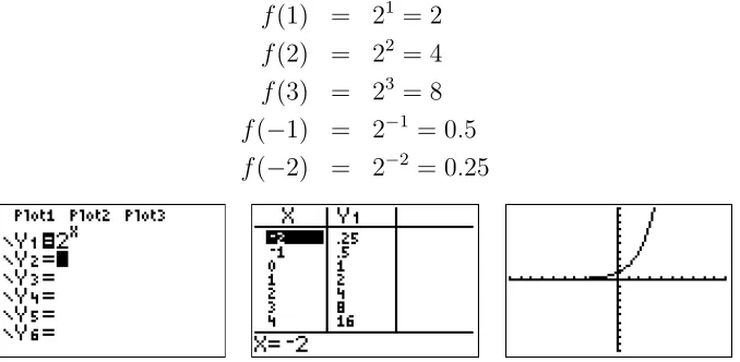
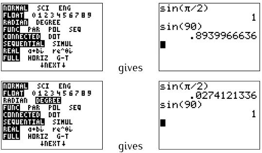
These are notes for a course in precalculus, as it is taught at New York City College of Technology - CUNY (where it is offered under the course number MAT 1375). Our approach is calculator based. For this, we will use the currently standard TI-84 calculator, and in particular, many of the examples will be explained and solved with it. However, we want to point out that there are also many other calculators that are suitable for the purpose of this course and many of these alternatives have similar functionalities as the calculator that we have chosen to use. An introduction to the TI-84 calculator together with the most common applications needed for this course is provided in appendix A. In the future we may expand on this by providing introductions to other calculators or computer algebra systems.
This course in precalculus has the overarching theme of “functions.” This means that many of the often more algebraic topics studied in the previous courses are revisited under this new function theoretic point of view. However, in order to keep this text as self contained as possible we always recall all results that are necessary to follow the core of the course even if we assume that the student has familiarity with the formula or topic at hand. After a first introduction to the abstract notion of a function, we study polynomials, ratio-nal functions, exponential functions, logarithmic functions, and trigonometric functions with the function viewpoint. Throughout, we will always place par-ticular importance to the corresponding graph of the discussed function which will be analyzed with the help of the TI-84 calculator as mentioned above. These are in fact the topics of the first four (of the five) parts of this precalculus course.
In the fifth and last part of the book, we deviate from the above theme and collect more algebraically oriented topics that will be needed in calculus or other advanced mathematics courses or even other science courses. This part includes a discussion of the algebra of complex numbers (in particular complex numbers in polar form), the 2-dimensional real vector space R2,
quences and series with focus on the arithmetic and geometric series (which are again examples of functions, though this is not emphasized), and finally the generalized binomial theorem.
In short, here is an outline of the topics in this course and the five parts into which this course is divided:
Part I: Functions and graphs
|
Part II: Polynomials and rational functions
|
Part III: Exponential and logarithmic functions
|
Part IV: Trigonometric functions
|
Part V: Complex numbers, sequences, and the binomial theorem
The topics in this book are organized in25sessions, each session correspond-ing to one class meetcorrespond-ing. Each session ends with a list of exercises that the student is expected to be able to solve. We cannot overstate the importance of completing these exercises for a successful completion of this course. These
25sessions, together with 4 scheduled exams and one review session give a total of 30 class sessions, which is the number of regularly scheduled class meetings in one semester. Each of the five parts also ends with a review of the topics discussed. This may be used as a review for any of the exams during the semester. Finally, we point out that there is an overview of the important formulas used in this course at the end of the book.
We would like to thank our colleagues and students for their support dur-ing the development of this project. In particular, we would like to thank Henry Africk, Johanna Ellner, Lin Zhou, Satyanand Singh, Jean Camilien, Leo Chosid, Laurie Caban, Natan Ovshey, Johann Thiel, Wendy Wang, Steven Karaszewski, Josue Enriquez, and Mohd Nayum Parvez, Akindiji Fadeyi, Is-abel Martinez, Erik Nowak, Sybil Shaver, Faran Hoosain, Kenia Rodriguez, Albert Jaradeh, Iftekher Hossain for many useful comments that helped to improve this text.
Thomas Tradler and Holly Carley
Preface iii
Table of contents v
I
Functions and graphs
1
1 The absolute value 2
1.1 Background regarding numbers . . . 2
1.2 The absolute value . . . 3
1.3 Inequalities and intervals . . . 4
1.4 Absolute value inequalities . . . 6
1.5 Exercises . . . 11
2 Lines and functions 13 2.1 Lines, slope and intercepts . . . 13
2.2 Introduction to functions . . . 22
2.3 Exercises . . . 28
3 Functions by formulas and graphs 32 3.1 Functions given by formulas . . . 32
3.2 Functions given by graphs . . . 37
3.3 Exercises . . . 44
4 Introduction to the TI-84 49 4.1 Graphing with the TI-84 . . . 49
4.2 Finding zeros, maxima, and minima . . . 53
4.3 Exercises . . . 61
5 Basic functions and transformations 63
5.1 Graphing basic functions . . . 63
5.2 Transformation of graphs . . . 65
5.3 Exercises . . . 73
6 Operations on functions 76 6.1 Operations on functions given by formulas . . . 76
6.2 Operations on functions given by tables . . . 81
6.3 Exercises . . . 83
7 The inverse of a function 86 7.1 One-to-one functions . . . 86
7.2 Inverse function . . . 88
7.3 Exercises . . . 95
Review of functions and graphs 98
II
Polynomials and rational functions
100
8 Dividing polynomials 101 8.1 Long division . . . 1028.2 Dividing by(x−c) . . . 106
8.3 Optional section: Synthetic division . . . 109
8.4 Exercises . . . 111
9 Graphing polynomials 113 9.1 Graphs of polynomials . . . 113
9.2 Finding roots of a polynomial with the TI-84 . . . 121
9.3 Optional section: Graphing polynomials by hand . . . 124
9.4 Exercises . . . 127
10 Roots of polynomials 130 10.1 Optional section: The rational root theorem . . . 130
10.2 The fundamental theorem of algebra . . . 134
11 Rational functions 147
11.1 Graphs of rational functions . . . 147 11.2 Optional section: Rational functions by hand . . . 159 11.3 Exercises . . . 168
12 Polynomial and rational inequalities 169
12.1 Polynomial inequalities . . . 169 12.2 Rational inequalities and absolute value inequalities . . . 176 12.3 Exercises . . . 179
Review of polynomials and rational functions 181
III
Exponential and logarithmic functions
183
13 Exponential and logarithmic functions 184
13.1 Exponential functions and their graphs . . . 184 13.2 Logarithmic functions and their graphs . . . 190 13.3 Exercises . . . 197
14 Properties of expand log 199
14.1 Algebraic properties of exp and log . . . 199 14.2 Solving exponential and logarithmic equations . . . 202 14.3 Exercises . . . 206
15 Applications of exp and log 208
15.1 Applications of exponential functions . . . 208 15.2 Exercises . . . 214
16 Half-life and compound interest 216
16.1 Half-life . . . 216 16.2 Compound interest . . . 220 16.3 Exercises . . . 226
IV
Trigonometric functions
231
17 Trigonometric functions 232
17.1 Basic trigonometric definitions and facts . . . 232 17.2 sin, cos, andtan as functions . . . 239 17.3 Exercises . . . 249
18 Addition of angles and multiple angles 252
18.1 Addition and subtraction of angles . . . 252 18.2 Double and half angles . . . 256 18.3 Exercises . . . 261
19 Inverse trigonometric functions 262
19.1 The functionssin−1, cos−1, andtan−1 . . . 262
19.2 Exercises . . . 269
20 Trigonometric equations 270
20.1 Basic trigonometric equations . . . 270 20.2 Equations involving trigonometric functions . . . 278 20.3 Exercises . . . 283
Review of trigonometric functions 284
V
Complex numbers, sequences, and the binomial theorem
286
21 Complex numbers 287
21.1 Polar form of complex numbers . . . 287 21.2 Multiplication and division of complex numbers . . . 294 21.3 Exercises . . . 297
22 Vectors in the plane 299
23 Sequences and series 311
23.1 Introduction to sequences and series . . . 311
23.2 The arithmetic sequence . . . 318
23.3 Exercises . . . 323
24 The geometric series 325 24.1 Finite geometric series . . . 325
24.2 Infinite geometric series . . . 330
24.3 Exercises . . . 334
25 The binomial theorem 337 25.1 The binomial theorem . . . 337
25.2 Binomial expansion . . . 342
25.3 Exercises . . . 345
Review of complex numbers, sequences, and the binomial theorem 347 A Introduction to the TI-84 349 A.1 Basic calculator functions . . . 349
A.2 Graphing a function . . . 353
A.2.1 Rescaling the graphing window . . . 354
A.3 Graphing more than one function . . . 357
A.4 Graphing a piecewise defined function . . . 359
A.5 Using the table . . . 361
A.6 Solving an equation using the solver . . . 362
A.7 Special functions (absolute value, n-th root, etc.) . . . 363
A.8 Programming the calculator . . . 366
A.9 Common errors . . . 370
A.10 Resetting the calculator to factory settings . . . 373
Answers to exercises 374 Session 1 . . . 374
Session 2 . . . 375
Session 3 . . . 375
Session 4 . . . 377
Session 5 . . . 379
Session 6 . . . 380
Review part I . . . 383
Session 8 . . . 383
Session 9 . . . 384
Session 10 . . . 385
Session 11 . . . 386
Session 12 . . . 388
Review part II . . . 389
Session 13 . . . 389
Session 14 . . . 392
Session 15 . . . 393
Session 16 . . . 393
Review part III . . . 393
Session 17 . . . 393
Session 18 . . . 396
Session 19 . . . 396
Session 20 . . . 397
Review part IV . . . 398
Session 21 . . . 398
Session 22 . . . 399
Session 23 . . . 400
Session 24 . . . 400
Session 25 . . . 401
Review part V . . . 401
References 402
Important formulas used in precalculus 403
Functions and graphs
Session 1
Absolute value equations and
inequalities
1.1
Background regarding numbers
Thenatural numbers (denoted by N) are the numbers
1,2,3,4,5, . . .
Theintegers (denoted by Z) are the numbers
. . . ,−4,−3,−2,−1,0,1,2,3,4,5, . . .
Therational numbers (denoted by Q) are the fractions ab of integersa and b
with b6= 0. Here are some examples of rational numbers:
3 5,−
2 6,17,0,
3 −8
Thereal numbers (denoted by R) are the numbers on the real number line
0 23 1
−√2 2 3 4
−2
−3 π
Here are some examples of real numbers:
√
3, π,−2
5,18,0,6.789
A real number that is not a rational number is called an irrational number. Here are some examples of irrational numbers:
π,√2,523, e
1.2
The absolute value
Theabsolute valueof a real numberc, denoted by|c|the non-negative number which is equal in magnitude (or size) to c, i.e., is the number resulting from disregarding the sign:
|c|=
c, ifc is positive or zero
−c, ifc is negative
Example 1.1. | −4|= 4
Example 1.2. |12|= 12
Example 1.3. | −3.523|= 3.523
Example 1.4. For which real numbers x do you have |x|= 3?
Solution. Since |3| = 3 and | −3| = 3, we see that there are two solutions,
x= 3 or x=−3. The solution set is S={−3,3}.
Example 1.5. Solve for x: |x|= 5
Solution. x= 5 or x=−5. The solution set is S ={−5,5}.
Example 1.6. Solve for x: |x|=−7.
Solution. Note that | − 7| = 7 and |7| = 7 so that these cannot give any solutions. Indeed, there are no solutions, since the absolute value is always non-negative. The solution set is the empty set S ={}.
Example 1.7. Solve for x: |x|= 0.
Solution. Since−0 = 0, there is only one solution,x= 0. Thus,S ={0}.
Solution. Since the absolute value of x+ 2 is6, we see that x+ 2 has to be either 6or −6. We evaluate each case,
either x+ 2 = 6, or x+ 2 =−6,
=⇒x= 6−2, =⇒x=−6−2,
=⇒x= 4; =⇒x=−8.
The solution set is S ={−8,4}.
Example 1.9. Solve forx: |3x−4|= 5
Solution.
Either 3x−4 = 5 or 3x−4 =−5
=⇒3x= 9 =⇒3x=−1
=⇒x= 3 =⇒x =−13
The solution set is S ={−13,3}.
Example 1.10. Solve forx: −2· |12 + 3x|=−18
Solution. Dividing both sides by −2 gives |12 + 3x|= 9. With this, we have the two cases
Either 12 + 3x= 9 or 12 + 3x=−9 =⇒3x=−3 =⇒3x=−21
=⇒x=−1 =⇒x =−7
The solution set is S ={−7,−1}.
1.3
Inequalities and intervals
There is an order relation on the set of real numbers:
4<9 reads as 4 is less than 9,
−3≤2 reads as −3 is less than or equal to 2,
7
6 >1 reads as 7
6 is greater than 1,
2≥ −3 reads as 2 is greater than or equal to −3.
Example 1.12. We have5≤5and5≥5. However the same is not true when using the symbol <. We write this as5≮5.
The set of all real numbers x greater than or equal to some number a
and/or less than or equal to some number b is denoted in different ways by the following chart:
Inequality notation Number line Interval notation
a≤x≤b a b [a, b]
a < x < b a b (a, b)
a≤x < b a b [a, b)
a < x≤b a b (a, b]
a≤x a [a,∞)
a < x a (a,∞)
x≤b b (−∞, b]
x < b b (−∞, b)
Formally, we define the interval [a, b] to be the set of all real numbersxsuch that a ≤x≤b:
[a, b] = { x | a≤x≤b }
There are similar definitions for the other intervals shown in the above table.
Warning1.13. Be sure to write the smaller numbera < bfirst when writing an interval[a, b]. For example, the interval[5,3] ={ x | 5≤x≤3 }would be the empty set!
Example 1.14. Graph the the inequality π < x≤ 5 on the number line and write it in interval notation.
Solution.
On the number line: π 5
Example 1.15. Write the following interval as an inequality and in interval
notation: −3
Solution.
Inequality notation: −3≤x
Interval notation: [−3,∞)
Example 1.16. Write the following interval as an inequality and in interval
notation: −1 0 1 2 3
Solution.
Inequality notation: x <2
Interval notation: (−∞,2)
Note1.17. In some texts round and square brackets are also used on the number line to depict an interval. For example the following displays the interval[2,5).
2 5
1.4
Absolute value inequalities
Using the notation from the previous section, we now solve inequalities in-volving the absolute value. These inequalities may be solved in three steps:
• Step 1: Solve the corresponding equality. The solution of the equality divides the real number line into several subintervals.
• Step 2: Using step 1, check the inequality for a number in each of the subintervals. This check determines the intervals of the solution set.
Here are some examples for the above solution method.
Example 1.18. Solve for x:
a) |x+ 7|<2 b) |3x−5| ≥11 c) |12−5x| ≤1
Solution. a) We follow the three steps described above. In step 1, we solve the corresponding equality, |x+ 7|= 2.
x+ 7 = 2 x+ 7 =−2 =⇒x=−5 =⇒x=−9
The solutions x = −5 and x =−9 divide the number line into three subin-tervals:
x <−9 −9< x <−5 −5< x
-13 -12 -11 -10 -9 -8 -7 -6 -5 -4 -3 -2 -1
Now, in step 2, we check the inequality for one number in each of these subintervals.
Check: x=−10 Check: x=−7 Check: x= 0 |(−10) + 7|<? 2 |(−7) + 7|<? 2 |0 + 7|<? 2
| −3|<? 2 |0|<? 2 |7|<? 2
3<? 2 0<? 2 7<? 2
false true false
Since x=−7in the subinterval given by −9< x <−5solves the inequality
|x+7|<2, it follows thatallnumbers in the subinterval given by−9< x < −5
solve the inequality. Similarly, since x = −10 and x = 0 do not solve the inequality, nonumber in these subintervals will solve the inequality. For step 3, we note that the numbersx=−9andx=−5are not included as solutions since the inequality is strict (that is we have <instead of≤).The solution set is therefore the interval S = (−9,−5). The solution on the number line is:
-13 -12 -11 -10 -9 -8 -7 -6 -5 -4 -3 -2 -1
b) We follow the steps as before. First, in step 1, we solve |3x−5|= 11.
The two solutions x = −2 and x = 163 = 513 divide the number line into the subintervals displayed below.
x <−2 −2< x <51
3 5
1 3 < x
-5 -4 -3 -2 -1 0 1 2 3 4 5 6 7 8 9
For step 2, we check a number in each subinterval. This gives:
Check: x=−3 Check: x= 1 Check: x= 6 |3·(−3)−5|≥? 11 |3·1−5|≥? 11 |3·6−5|≥? 11
| −9−5|≥? 11 |3−5|≥? 11 |18−5|≥? 11
| −14|≥? 11 | −2|≥? 11 |13|≥? 11
14≥? 11 2≥? 11 13≥? 11
true false true
For step 3, note that we include −2 and 513 in the solution set since the inequality is “greater than or equal to” (that is ≥, as opposed to >). Furthermore, the numbers −∞ and ∞ are not included, since ±∞ are not real numbers.
The solution set is therefore the union of the two intervals:
S =− ∞,−2i∪h51 3,∞
c) To solve |12−5x| ≤1, we first solve the equality|12−5x|= 1.
12−5x= 1 12−5x=−1
=⇒ −5x=−11 =⇒ −5x=−13 =⇒x= −−115 = 2.2 =⇒x= −−135 = 2.6
Interval: x <2.2 Interval: 2.2< x <2.6 Interval: 2.6< x
Check: x= 1 Check: x= 2.4 Check: x= 3
|12−5·1|≤? 1 |12−5·2.4|≤? 1 |12−5·3|≤? 1
|12−5|≤? 1 |12−12|≤? 1 |12−15|≤? 1
|7|≤? 1 |0|≤? 1 | −3|≤? 1
7≤? 1 0≤? 1 3≤? 1
false true false
The solution set is the intervalS = [2.2,2.6], where we included x = 2.2
and x= 2.6since the original inequality “less than or equal to” (≤) includes the equality.
Note: Alternatively, whenever you have an absolute value inequality you can turn it into two inequalities. Here are a couple of examples.
Example 1.19. Solve for x: |12−5x| ≤1
Solution. Note that|12−5x| ≤1 implies that
−1≤12−5x≤1
so that
−13≤ −5x≤ −11
and by dividing by−5(remembering to switch the direction of the inequalities when multiplying or dividing by a negative number) we see that
13
5 ≥x≥ 11
5 ,
or in interval notation, we have the solution set
S=
11 5 ,
13 5
.
Example 1.20. If |x+ 6| > 2 then either x + 6 > 2 or x + 6 < −2 so that either x > −4 or x < −8 so that in interval notation the solution is
Observation 1.21. There is a geometric interpretation of the absolute value on the number line as the distance between two numbers:
distance between a and b is|b−a| which is also equal to |a−b|
a b
This interpretation can also be used to solve absolute value equations and inequalities.
Example 1.22. Solve forx: a) |x−6|= 4, b)|x−6| ≤4, c)|x−6| ≥4.
Solution. a) Consider the distance betweenxand6to be4on a number line:
-3 -2 -1 0 1 2 3 4 5 6 7 8 9 10 11 12
distance4 distance4
There are two solutions, x = 2 or x = 10. That is, the distance between 2
and6 is 4 and the distance between 10 and6 is 4.
b) Numbers inside the braces above have distance4 or less. The solution is given on the number line as:
-3 -2 -1 0 1 2 3 4 5 6 7 8 9 10 11 12
distance≤4 distance≤4
In interval notation, the solution set is the intervalS = [2,10]. One can also write that the solution set consists of all x such that2≤x≤10.
c) Numbers outside the braces above have distance4or more. The solution is given on the number line as:
-3 -2 -1 0 1 2 3 4 5 6 7 8 9 10 11 12
distance<4 distance<4
In interval notation, the solution set is the interval(−∞,2]and[10,∞), or in short it is the union of the two intervals:
One can also write that the solution set consists of all x such that x ≤2 or
x≥10.
1.5
Exercises
Exercise 1.1. Give examples of numbers that are
a) natural numbers b) integers c) integers but not natural numbers d) rational numbers e) real numbers f) rational numbers but not integers
Exercise 1.2. Which of the following numbers are natural numbers, integers, rational numbers, or real numbers? Which of these numbers are irrational?
a) 7
3 b) −5 c) 0 d) 17,000 e)
12
4 f)
√
7 g)√25
Exercise 1.3. Evaluate the following absolute value expressions:
a) | −8|, b) |10|, c) | −99|, d) −|3|, e) −| −2|, f) | −√6|, g) |3 + 4|, h) |2−9|, i) | −5.4|, j) −2
3
, k) 5
−2
, l) −−−6
−3
.
Exercise 1.4. Solve forx:
a) |x|= 8 b) |x|= 0 c) |x|=−3
d) |x+ 3|= 10 e) |2x+ 5|= 9 f)|2−5x|= 22
g) |4x|=−8 h) | −7x−3|= 0 i)|4−4x| = 44
j) −2· |2−3x|=−12 k) 5 +|2x+ 7|= 14 l)−| −8−2x|=−12
Exercise 1.5. Solve for x using the geometric interpretation of the absolute value:
a)|x|= 8 b) |x|= 0 c) |x|=−3
Exercise 1.6. Complete the table.
Inequality notation Number line Interval notation
2≤x <5
x≤3
12 17
−2
[−2,6] (−∞,0)
4.5 5< x≤√30
(137 , π)
Exercise 1.7. Solve forx and write the solution in interval notation. a)|x−4| ≤7 b) |x−4| ≥7 c) |x−4|>7
d) |2x+ 7| ≤13 e) | −2−4x|>8 f) |4x+ 2|<17
g)|15−3x| ≥6 h) 5x−4
3
> 2
3 i)
Lines and functions
2.1
Lines, slope and intercepts
In this chapter we will introduce the notion of a function. Before we give the general definition, we recall one special kind of function which is already familiar to the student. More precisely, we start by recalling functions that are given by straight lines.
We have seen in the last section that each point on the number line is represented by a real number xin R. Similarly, each point in the coordinate plane is represented by a pair of real numbers (x, y). The coordinate plane is denoted by R2. Here is a picture of the coordinate plane:
-3 -2 -1 0 1 2 3
-3 -2 -1 0 1 2 3
x y
In this section, we will discuss the straight line in the coordinate plane. We will discuss its slope and intercepts. We will also discuss the line’s
corresponding algebraic forms: the point-slope form and the slope-intercept form.
By drawing a line on a coordinate plane we associate every point on the line with a pair of numbers (a, b), where a is called the x−coordinate and b
is called the y−coordinate. Consider, for example, the picture
-5 -4 -3 -2 -1 0 1 2 3 4
-1 0 1 2 3 4
x y
x y
L
We see that(−2,0)lies on the line and so does(2,2). Of course, there are an infinite number of points on the line. This set of points can also be described by an equation relating thex− andy−coordinates of points on the line. For example 2y−x = 2 is the equation of the line above. Notice that (−2,0)
satisfies the equation since2(0)−(−2) = 2 and(2,2) satisfies the equation since 2(2)−(2) = 2. It is a fact that every line has an equation of the form
px+qy=r, that is, given a line, there are numbersp, qandr so that a point
(a, b) is on the graph of the line if and only if pa+qb=r.
Notice that, in the example, if we put our finger on(−2,0)and move it up and over to the point(2,2)we have moved2units up and4 units to the right. If from there ((2,2)) we move another 2 units up and4units to the right then we land again on the line (at (6,4)). In fact no matter where we start on the line if from there we move2 units up and4 units to the right we always land on the line again. The ratio rise
run =
2
4 is called theslope of this line. The word
‘rise’ indicates vertical movement (down being negative) and ‘run’ indicates horizontal movement (left being negative). Notice that 24 = 12 = −−12 and so on. So we could also see that if we start at (−2,0) and rise 1 and run 2we land at(0,1)which is on the line and if we start at (2,2)and rise −1(move down 1) and run −2 (move to the left 2) we end up at (0,1), which is again on the line.
given by the following formula (which is riserun):
x y
P2
P1
x1 x2
y1 y2
Slope: m= y2−y1
x2−x1
(2.1)
The slope determines how fast a line grows. When the slope m is negative the line declines towards the right.
x y
x y
x y
x y
x y
m = 2 m= 12 m= 0 m=−12 m=−2
From equation (2.1), we see that for a given slopemand a pointP1(x1, y1)
on the line, any other point(x, y)on the line satisfiesm= y−y1
x−x1. Multiplying (x−x1) on both sides gives what is called thepoint-slope form of the line:
y−y1 =m·(x−x1) (2.2)
x y
L
y-intercept x-intercept
One way to describe a line using the slope and y-intercept is the so-called slope-intercept form of the line.
Definition 2.1. The slope-intercept form of the lineis the equation
y=m·x+b (2.3)
Here, m is the slope and (0, b) is they-intercept of the line. Here is an example of a line in slope-intercept form.
Example 2.2. Graph the line y= 2x+ 3.
Solution. We calculate y for various values of x. For example, when x is
−2,−1,0,1,2, or 3, we calculate
x −2 −1 0 1 2 3
y −1 1 3 5 7 9
In the above table eachyvalue is calculated by substituting the corresponding
x value into our equationy = 2x+ 3:
x=−2 =⇒ y= 2·(−2) + 3 =−4 + 3 =−1
x=−1 =⇒ y= 2·(−1) + 3 =−2 + 3 = 1
x= 0 =⇒ y= 2·(0) + 3 = 0 + 3 = 3
x= 1 =⇒ y= 2·(1) + 3 = 2 + 3 = 5
x = 2 =⇒ y= 2·(2) + 3 = 4 + 3 = 7
x = 3 =⇒ y= 2·(3) + 3 = 6 + 3 = 9
In the above calculation, the values for x were arbitrarily chosen. Since a line is completely determined by knowing two points on it, any two values for
Drawing the above points in the coordinate plane and connecting them gives the graph of the line y= 2x+ 3:
-4 -3 -2 -1 0 1 2 3 4
-2 -1 0 1 2 3 4 5 6 7 8 9 10
x y
Alternatively, note that the y-intercept is (0,3) (3 is the additive constant in our initial equation y= 2x+ 3) and the slope m= 2 determines the rate at which the line grows: for each step to the right, we have to move two steps up.
To plot the graph, we first plot the y-intercept (0,3). Then from that point, rise 2 and run 1 so that you find yourself at (1,5) (which must be on the graph), and similarly rise 2 and run 1 to get to (2,7) (which must be on the graph), etc. Plot these points on the graph and connect the dots to form a straight line. As noted above, any2 distinct points on the graph of a straight line are enough to plot the complete line.
Proof that (0, b) is the y-intercept, and m is the slope.
Given the line y = mx+b, we want to calculate its y-intercept and its slope. They-intercept is the value ofy where x= 0. Therefore, we have that the y−coordinate of they-intercept is
y=m·0 +b=b.
This shows the first claim.
Next, to see why m is the slope, note that P1(x1, y1) lies on the line
exactly wheny1 =mx1+b. Similarly,P2(x2, y2)lies on the line exactly when y2 =mx2+b. Subtracting y1 =mx1+b from y2 =mx2+b, we obtain:
y2−y1 = (mx2+b)−(mx1+b) =mx2+b−mx1−b =m·(x2−x1).
Dividing by (x2−x1) gives y2−y1 (x2−x1)
= m·(x2 −x1) (x2−x1)
= m
1 =m.
By Equation (2.1) the fraction y2−y1
x2−x1 is the slope, establishing that our m is
indeed the slope, as we claimed.
Example 2.3. Find the equation of the line in slope-intercept form.
-4 -3 -2 -1 0 1 2 3 4 5 6 -2
-1 0 1 2 3 4 5
x y
Solution. They-intercept can be read off the graph giving us thatb = 2. As for the slope, we use formula (2.1) and the two points on the lineP1(0,2)and P2(4,0). We obtain
m= 0−2 4−0 =
−2
4 =−
1 2.
Example 2.4. Find the equation of the line in slope-intercept form.
-6 -5 -4 -3 -2 -1 0 1 2 3 4 5 6
-7 -6 -5 -4 -3 -2 -1 0 1
x y
Solution. The y-intercept is b =−4. To obtain the slope we can again use the y-interceptP1(0,−4). To use (2.1), we need another pointP2 on the line.
We may pick any second point on the line, for example,P2(3,−3). With this,
we obtain
m= (−3)−(−4)
3−0 =
−3 + 4
3 =
1 3.
Thus, the line has the slope-intercept form y= 1 3x−4.
Example 2.5. Find the equation of the line in point-slope form (2.2).
-1 0 1 2 3 4 5 6 7 8 9 10 11 12 -1
0 1 2 3 4 5
x y
Solution. We need to identify one point (x1, y1) on the line together with
the slope m of the line so that we can write the line in point-slope form:
y−y1 =m(x−x1). By direct inspection, we identify the two points P1(5,1)
and P2(8,3) on the line, and with this we calculate the slope as
m = 3−1 8−5 =
Using the point (5,1) we write the line in point-slope form as follows:
y−1 = 2
3(x−5)
Note that our answer depends on the chosen point(5,1)on the line. Indeed, if we choose a different point on the line, such as (8,3), we obtain a different equation, (which nevertheless represents the same line):
y−3 = 2
3(x−8)
Note, that we do not need to solve this for y, since we are looking for an answer in point-slope form.
Example 2.6. Find the slope, find they-intercept, and graph the line
4x+ 2y−2 = 0.
Solution. We first rewrite the equation in slope-intercept form.
4x+ 2y−2 = 0 (−=4⇒x+2) 2y=−4x+ 2 (divide2)
=⇒ y=−2x+ 1
We see that the slope is −2and the y-intercept is (0,1).
We can then plot they−intercept(0,1)and use the slope m= −12 to find another point (1,−1). Plot that point, connect the two plotted points, and extend to see the graph below.
We can also graph by plotting points. We can calculate the y-values for some x-values. For example when x=−2,−1, . . . ,3, we obtain:
x −2 −1 0 1 2 3
This gives the following graph:
-5 -4 -3 -2 -1 0 1 2 3 4 5
-5 -4 -3 -2 -1 0 1 2 3 4 5
x y
Example 2.7. Find the slope,y-intercept, and graph the line5y+ 2x=−10.
Solution. Again, we first rewrite the equation in slope-intercept form.
5y+ 2x=−10 (subtract=⇒2x) 5y=−2x−10 (divide5)
=⇒ y= −2x−10 5
=⇒ y=−2
5x−2
Now, the slope is −25 and the y-intercept is (0,−2).
We can plot they−intercept and from there move2units down and5units to the right to find another point on the line. The graph is given below.
To graph it by plotting points we need to find points on the line. In fact, any two points will be enough to completely determine the graph of the line. For some “smart” choices of x or y the calculation of the corresponding value may be easier than for others. We suggest that you find the x− and
y−intercepts, i.e., point of the form (?,0) (y = 0 in the equation and find
x) and (0,?) (set x = 0 in the equation and find y). Plugging x = 0 into
5y+ 2x=−10, we obtain
x=0
Similarly, substitutingy= 0 into 5y+ 2x=−10gives
y=0
=⇒ 5·0 + 2x=−10 =⇒ 2x=−10 =⇒ x=−5.
We obtain the following table:
x 0 −5
y −2 0
This gives the following graph:
-8 -7 -6 -5 -4 -3 -2 -1 0 1 2 3
-3 -2 -1 0 1
x y
2.2
Introduction to functions
We now formally introduce the notion of a function. A first example was provided by a straight line such as, for example, y = 5x+ 4. Note, that for each given x we obtain an induced y. (For example, for x = 3, we obtain
y= 5·3 + 4 = 19.)
Definition 2.8. A function f consists of two sets, a set D of inputs called the domain and a set C of possible outputs called the codomain, and an assignment that assigns to each inputx exactly one output y.
A function f with domainD and codomain C is denoted by
f :D→C.
If x is in the domain D (an input), then we denote by f(x) = y the output that is assigned byf tox.
Definition2.9. Therange Rof a functionf is a subset of the codomain given by R = {f(x)|x in the domain of f}. That is, the range is the set of all outputs.
Warning2.10. Some authors use a slightly different convention by calling the range what we called the codomain above.
Since we will be dealing with many functions it is convenient to name vari-ous functions (usually with lettersf, g, h, etc). Often we will implicitly assume that a domain and codomain are given without specifying these explicitly. If the range can be determined and the codomain is not given explicitly, then we take the codomain to be the range. If the range can not easily be determined and the codomain is not explicitly given, then the codomain should be taken to be a ‘simple’ set which clearly contains the range.
There are several ways to represent a particular function (all of which may not apply to a specific function): via a table of values (listing the input-output pairs), via a formula (with the domain and range explicitly or implicitly given), via a graph (representing input-output pairs on a coordinate plane), or in words, just to name a few. We have seen examples of the first three of these in previous sections. Our discussion in this section goes into greater detail.
Example 2.11. Define the assignment f by the following table
x 2 5 −3 0 7 4
y 6 8 6 4 −1 8
The assignment f assigns to the input 2 the output 6, which is also written as
f(2) = 6.
Similarly, f assigns to 5the number 8, in short f(5) = 8, etc:
f(5) = 8, f(−3) = 6, f(0) = 4, f(7) =−1, f(4) = 8.
The domain D is the set of all inputs. The domain is therefore
The range R is the set of all outputs. The range is therefore
R={−1,4,6,8}.
The assignmentf is indeed a function since each element of the domain gets assigned exactly one element in the range. Note that for an input number that is not in the domain, f does not assign an output to it. For example,
f(1) =undefined.
Note also that f(5) = 8 and f(4) = 8, so that f assigns to the inputs 5
and 4 the same output 8. Similarly, f also assigns the same output to the inputs2 and −3. Therefore we see that:
• A function may assign the same output to two different inputs!
Example2.12. Consider the assignmentf that is given by the following table.
x 2 5 −3 0 5 4
y 6 8 6 4 −1 8
This assignment does not define a function! What went wrong?
Consider the input value5. What does f assign to the input 5? The third column states that f assigns to 5 the output 8, whereas the sixth column states thatf assigns to 5 the output −1,
f(5) = 8, f(5) =−1.
However, by the definition of a function, to each input we have to assign exactly one output. So, here, to the input 5 we have assigned two outputs 8
and−1. Therefore, f is not a function.
• A function cannot assign two outputs to one input!
We repeat the two bullet points from the last two examples, which are crucial for the understanding of a function.
Note 2.13.
• A function may assign the same output to two different inputs!
• A function cannot assign two outputs to one input!
f(x) =y1 and f(x) =y2 with y1 6=y2 is not allowed!
Example2.14. A university creates a mentoring program, which matches each freshman student with a senior student as his or her mentor. Within this pro-gram it is guaranteed that each freshman gets precisely one mentor, however two freshmen may receive the same mentor. Does the assignment of freshmen to mentor, or mentor to freshmen describe a function? If so, what is its domain, what is its range?
Solution. Since a senior may mentor several freshman, we cannot take a mentor as an “input,” as he or she would be assigned to several “output” freshmen students. So freshman is not a function of mentor.
On the other hand, we can assign each freshmen to exactly one mentor, which therefore describes a function. The domain (the set of all inputs) is given by the set of all freshmen students. The range (the set of all outputs) is given by the set of all senior students that are mentors. The function assigns each “input” freshmen student to his or her unique “output” mentor.
Example 2.15. The rainfall in a city for each of the 12 months is displayed in the following histogram.
ra
inf
a
ll
[in] ✻
✲ J F MA MJ J A S O N D month
a) Is the rainfall a function of the month?
b) Is the month a function of the rainfall?
Solution.
b) If we take a certain rainfall amount as our input data, can we associate a unique month to it? For example, February and March have the same amount of rainfall. Therefore, to one input amount of rainfall we cannot assign a unique month. The month isnot a function of the rainfall.
Example 2.16. Consider the functionf described below.
△ ♦
yellow
green
blue
f
Here, the functionf maps the input symbolto the output color blue. Other
assignments off are as follows:
f() =blue, f(△) =yellow
f(♦) =green, f() =yellow
The domain is the set of symbols D = {,△,♦,}, and the range is the set of colorsR={blue,green,yellow}. Notice, in particular, that the inputs
△and both have the same output yellow, which is certainly allowed for a function.
Example2.17. Consider the functiony = 5x+4with domain all real numbers and range all real numbers. Note that for each inputx, we obtain an exactly one induced output y. For example, for the input x = 3 we get the output
y= 5·3 + 4 = 19, etc.
Example 2.18. Consider the function y = x2 with domain all real numbers
Example 2.19. For each real number x, denote by ⌊x⌋ the greatest integer that is less or equal tox. We call⌊x⌋thefloor ofx. For example, to calculate
⌊4.37⌋, note that all integers 4,3,2, . . . are less or equal to 4.37:
. . . ,−3,−2,−1,0,1,2,3,4 ≤ 4.37
The greatest of these integers is 4, so that ⌊4.37⌋ = 4. We define the floor function as f(x) = ⌊x⌋. Here are more examples of function values of the floor function.
⌊7.3⌋= 7, ⌊π⌋= 3, ⌊−4.65⌋=−5,
⌊12⌋= 12,
−26 3
=⌊−8.667⌋=−9
The domain of the floor function is the set of all real numbers, that is D=R. The range is the set of all integers, R =Z.
Example 2.20. LetAbe the area of an isosceles right triangle with base side length x. Express A as a function of x.
Solution. Being an isosceles right triangle means that two side lengths are
x, and the angles are 45◦, 45◦, and90◦ (or in radian measure π
4,
π
4, and
π
2):
x x
Recall that the area of a triangle is: area = 1
2 base· height. In this case, we
have base=x, and height=x, so that the area
A= 1
2x·x= 1 2x
2.
Example 2.21. Consider the equation y = x2+ 3. This equation associates
to each input numbera exactly one output numberb =a2+ 3. Therefore, the
equation defines a function. For example:
To the input5 we assign the output 52+ 3 = 25 + 3 = 28.
The domain D is all real numbers, D = R. Since x2 is always ≥ 0, we
see that x2 + 3 ≥ 3, and vice versa every number y ≥ 3 can be written as y=x2 + 3. (To see this, note that the input x =√y−3 for y ≥3 gives the
output x2 −3 = (√y−3)2 + 3 = y −3 + 3 = y.) Therefore, the range is R= [3,∞).
Example2.22. Consider the equationx2+y2 = 25. Does this equation define yas a function ofx? That is, does this equation assign to each inputxexactly one outputy?
An input numberx gets assigned to y with x2+y2 = 25. Solving this for y, we obtain
y2 = 25−x2 =⇒ y=±√25−x2.
Therefore, there are two possible outputs associated to the input x(6= 5):
either y= +√25−x2 or y=−√25−x2.
For example, the input x = 0 has two outputs y = 5 and y =−5. However, a function cannot assign two outputs to one input x! The conclusion is that
x2+y2 = 25 does not determine y as a function!
Note 2.23. Note that if y =f(x) then x is called the independent variable
and y is called the dependent variable (since it depends on x). If x = g(y)
then y is the independent variable and x is the dependent variable (since it depends ony).
2.3
Exercises
slope-intercept form.
a)
-5 -4 -3 -2 -1 0 1 2 3 4 5
-5 -4 -3 -2 -1 0 1 2 3 4 5 x y b)
-5 -4 -3 -2 -1 0 1 2 3 4 5
-5 -4 -3 -2 -1 0 1 2 3 4 5 x y c)
-5 -4 -3 -2 -1 0 1 2 3 4 5
-5 -4 -3 -2 -1 0 1 2 3 4 5 x y d)
-5 -4 -3 -2 -1 0 1 2 3 4 5
-2 -1 0 1 2 3 4 5 6 x y e)
-4 -3 -2 -1 0 1 2 3 4
-4 -3 -2 -1 0 1 2 3 4 x y f)
-8 -7 -6 -5 -4 -3 -2 -1 0 1 2
-2 -1 0 1 2 3 4 5 6 x y
Exercise 2.2. Write the equation of the line in slope-intercept form. Identify slope and y-intercept of the line.
a)4x+ 2y= 8 b) 9x−3y+ 15 = 0 c) −5x−10y= 20
Exercise2.3. Find the equation of the line in point-slope form (2.2) using the indicated point P1.
a)
-1 0 1 2 3 4 5 6 7 8
-1 0 1 2 3 4 5 x y P1 b)
-1 0 1 2 3 4 5 6 7 8
-2 -1 0 1 2 3 4 x y P1 c)
-5 -4 -3 -2 -1 0 1 2 3 4 5
-4 -3 -2 -1 0 1 2 3 x y P1 d)
-6 -5 -4 -3 -2 -1 0 1 2 3
-3 -2 -1 0 1 2 3 4 x y P1
Exercise2.4. Graph the line by calculating a table (as in Example 2.2). (Solve fory first, if this is necessary.)
a)y= 2x−4 b) y=−x+ 4 c) y= 1 2x+ 1
d) y= 3x e) 8x−4y= 12 f)x+ 3y+ 6 = 0
Exercise 2.5. Determine if the given table describes a function. If so, deter-mine its domain and range. Describe which outputs are assigned to which inputs.
a)
x −5 3 −1 6 0
y 5 2 8 3 7
b)
x 6 17 4 −2 4
y 8 −2 0 3 −1
c)
x 19 7 6 −2 3 −11
d)
x 1 2 3 3 4 5
y 5.33 9 13 13 17 √19
e)
x 0 1 2 2 3 4
y 0 1 2 3 3 4
Exercise 2.6. We consider children and their (birth) mothers.
a) Does the assignment child to their birth mother constitute a function (in the sense of Definition 2.8 on page 22)?
b) Does the assignment mother to their children constitute a function? c) In the case where the assignment is a function, what is the domain? d) In the case where the assignment is a function, what is the range?
Exercise 2.7. A bank offers wealthy customers a certain amount of interest, if they keep more than 1 million dollars in their account. The amount is described in the following table.
dollar amount x in the account interest amount
x≤$1,000,000 $0
$1,000,000< x≤$10,000,000 2% of x
$10,000,000< x 1% of x
a) Justify that the assignment cash amount to interest defines a function. b) Find the interest for an amount of:
i)$50,000 ii) $5,000,000 iii)$1,000,000
iv)$30,000,000 v) $10,000,000 vi)$2,000,000
Exercise 2.8. Find a formula for a function describing the given inputs and outputs.
a) input: the radius of a circle,
output: the circumference of the circle
b) input: the side length in an equilateral triangle, output: the perimeter of the triangle
c) input: one side length of a rectangle, with other side length being 3, output: the perimeter of the rectangle
Session 3
Functions by formulas and graphs
3.1
Functions given by formulas
Most of the time we will discuss functions that take some real numbers as inputs, and give real numbers as outputs. These functions are commonly described with a formula.
Example 3.1. For the given function f, calculate the outputs f(2), f(−3), andf(−1).
a) f(x) = 3x+ 4, b) f(x) =√x2−3,
c) f(x) =
5x−6 , for −1≤x≤1
x3+ 2x , for 1< x≤5 d) f(x) = xx+2+3.
Solution. We substitute the input values into the function and simplify.
a) f(2) = 3·2 + 4 = 6 + 4 = 10, f(−3) = 3·(−3) + 4 =−9 + 4 =−5, f(−1) = 3·(−1) + 4 =−3 + 4 = 1.
b) Similarly, we calculate
f(2) = √22−3 =√4−3 = √1 = 1, f(−3) = p(−3)2−3 =√9−3 =√6,
f(−1) = p(−1)2−3 =√1−3 =√−2 =undefined.
For the last step, we are assuming that we only deal with real numbers. Of course, as we will see later on, √−2 can be defined as a complex number. But for now, we will only allow real solutions outputs.
c) The function f(x) =
5x−6 , for −1≤x≤1
x3+ 2x , for 1< x≤5 is given as a
piece-wise defined function. We have to substitute the values into the correct branch:
f(2) = 23+ 2·2 = 8 + 4 = 12, since 1<2≤5,
f(−3) = undefined, since −3is not in any of the two branches, f(−1) = 5·(−1)−7 =−5−6 =−11, since −1≤ −1≤1.
d) Finally for f(x) = x+2
x+3, we have:
f(2) = 2 + 2 2 + 3 =
4 5,
f(−3) = −3 + 2 −3 + 3 =
−1
0 =undefined,
f(−1) = −1 + 2 −1 + 3 =
1 2.
Example 3.2. Let f be the function given by f(x) =x2 + 2x−3. Find the
following function values.
a)f(5) b) f(2) c) f(−2) d) f(0)
e) f(√5) f) f(√3 + 1) g) f(a) h) f(a) + 5
i)f(x+h) j) f(x+h)−f(x) k) f(x+hh)−f(x) l) f(xx)−−fa(a)
Solution. The first four function values ((a)-(d)) can be calculated directly:
f(5) = 52+ 2·5−3 = 25 + 10−3 = 32, f(2) = 22+ 2·2−3 = 4 + 4−3 = 5,
f(−2) = (−2)2+ 2·(−2)−3 = 4 +−4−3 =−3, f(0) = 02+ 2·0−3 = 0 + 0−3 =−3.
The next two values ((e) and (f)) are similar, but the arithmetic is a bit more involved.
f(√3 + 1) = (√3 + 1)2+ 2·(√3 + 1)−3
= (√3 + 1)·(√3 + 1) + 2·(√3 + 1)−3 = √3·√3 + 2·√3 + 1·1 + 2·√3 + 2−3 = 3 + 2·√3 + 1 + 2·√3 + 2−3
= 3 + 4·√3.
The last five values ((g)-(l)) are purely algebraic:
f(a) = a2+ 2·a−3,
f(a) + 5 = a2+ 2·a−3 + 5 =a2+ 2·a+ 2, f(x+h) = (x+h)2+ 2·(x+h)−3
= x2+ 2xh+h2+ 2x+ 2h−3,
f(x+h)−f(x) = (x2+ 2xh+h2+ 2x+ 2h−3)−(x2+ 2x−3) = x2+ 2xh+h2+ 2x+ 2h−3−x2−2x+ 3 = 2xh+h2+ 2h,
f(x+h)−f(x)
h =
2xh+h2 + 2h h
= h·(2x+h+ 2)
h = 2x+h+ 2,
and
f(x)−f(a)
x−a =
(x2+ 2x−3)−(a2+ 2a−3) x−a
= x
2+ 2x−3−a2−2a+ 3
x−a =
x2−a2+ 2x−2a x−a
= (x+a)(x−a) + 2(x−a)
x−a =
(x−a)(x+a+ 2)
(x−a) =x+a+ 2.
The quotients f(x+hh)−f(x) and f(xx)−−fa(a) as in the last two examples 3.2(k) and (l) will become particularly important in calculus. They are called differ-ence quotients. We now calculate some more examples of difference quotients.
Example 3.3. Calculate the difference quotient f(x+hh)−f(x) for
a)f(x) =x3+ 2, b) f(x) = 1
Solution. We calculate first the difference quotient step by step.
a) f(x+h) = (x+h)3+ 2 = (x+h)·(x+h)·(x+h) + 2 = (x2+ 2xh+h2)·(x+h) + 2
=x3+ 2x2h+xh2+x2h+ 2xh2+h3 + 2,
=x3+ 3x2h+ 3xh2+h3+ 2.
Subtracting f(x) fromf(x+h) gives
f(x+h)−f(x) = (x3+ 3x2h+ 3xh2+h3+ 2)−(x3+ 2) =x3+ 3x2h+ 3xh2+h3+ 2−x3 −2 = 3x2h+ 3xh2+h3.
With this we obtain:
f(x+h)−f(x)
h =
3x2h+ 3xh2+h3 h
= h·(3x
2+ 3xh+h2)
h = 3x
2+ 3xh+h2.
We handle part (b) similarly.
b) f(x+h) = 1
x+h,
so that
f(x+h)−f(x) = 1
x+h −
1
x.
We obtain the solution after simplifying the double fraction:
f(x+h)−f(x)
h =
1
x+h −
1
x
h =
x−(x+h) (x+h)·x
h =
x−x−h
(x+h)·x
h =
−h
(x+h)·x
h
= −h
(x+h)·x·
1
h =
−1 (x+h)·x.
Convention3.4. Unless otherwise stated, a functionf has the largest possible domain, that is the domain is the set of all real numbersxfor which f(x)is a well-defined real number. We refer to this as thestandard convention of the domain. (In particular, under this convention, any polynomial has the domain R of all real numbers.)
The range is the set of all outputs obtained byf from the inputs (see also the warning on page 23.)
Example 3.5. Find the domain of each of the following functions.
a) f(x) = 4x3 −2x+ 5, b)f(x) =|x|,
c) f(x) =√x, d) f(x) =√x−3, e) f(x) = x1, f)f(x) = x2+8x−x2+15,
g) f(x) =
x+ 1 , for 2< x≤4 2x−1 , for 5≤x
Solution.
a) There is no problem taking a real number x to any (positive) power. Therefore,f is defined for all real numbersx, and the domain is written asD=R.
b) Again, we can take the absolute value for any real number x. The domain is all real numbers, D=R.
c) The square root √x is only defined for x ≥ 0 (remember we are not using complex numbers yet!). Thus, the domain is D= [0,∞).
d) Again, the square root is only defined for non-negative numbers. Thus, the argument in the square root has to be greater or equal to zero:
x−3≥0. Solving this for x gives
x−3≥0 (add=⇒3) x≥3.
The domain is therefore,D = [3,∞).
f) Again, we need to make sure that the denominator does not become zero; however we do not care about the numerator. The denominator is zero exactly when x2 + 8x+ 15 = 0. Solving this for x gives:
x2+ 8x+ 15 = 0 =⇒ (x+ 3)·(x+ 5) = 0 =⇒ x+ 3 = 0 or x+ 5 = 0 =⇒ x=−3or x=−5.
The domain is all real numbers except for −3 and −5, that is D =
R− {−5,−3}.
g) The function is explicitly defined for all2< x≤4and5≤x. Therefore, the domain is D= (2,4]∪[5,∞).
3.2
Functions given by graphs
In many situations, a function is represented by its graph. The graph of a function f is the set of all points (on the coordinate plane) of the form
(x, f(x)), where x is in the domain of f. We have already seen an example of graphing a function when we discussed lines and their graphs. Here is another example that shows how the formulaic definition relates to the graph of the function.
Example3.6. Lety=x2with domainD=Rbeing the set of all real numbers.
We can graph this after calculating a table as follows:
x −3 −2 −1 0 1 2 3
y 9 4 1 0 1 4 9
-5 -4 -3 -2 -1 0 1 2 3 4 5 -1
0 1 2 3 4 5 6 7 8 9 10
x y
P(2,4)
x= 2input y= 4
Many function values can be read from this graph. For example, for the input
x= 2, we obtain the output y = 4. This corresponds to the point P(2,4)on the graph as depicted above.
In general, an input (placed on the x-axis) gets assigned to an output (placed on the y-axis) according to where the vertical line at x intersects with the given graph. This is used in the next example.
Example 3.7. Letf be the function given by the following graph.
-1 0 1 2 3 4 5 6 7 8 9 10 -1
0 1 2 3 4 5
x y
Here, the dashed lines show, that the input x = 3 gives an output of y = 2. Similarly, we can obtain other output values from the graph:
f(2) = 4, f(3) = 2, f(5) = 2, f(7) = 4.
Note, that in the above graph, a closed point means that the point is part of the graph, whereas an open point means that it is not part of the graph.
The domain is the set of all possible input values on the x-axis. Since we can take any number 2 ≤ x ≤ 7 as an input, the domain is the interval
Example 3.8. Let f be the function given by the following graph.
-6 -5 -4 -3 -2 -1 0 1 2 3 4 5 6
-2 -1 0 1 2 3 4
x y
Here are some function values that can be read from the graph:
f(−5) = 2, f(−4) = 3, f(−3) and f(−2) are undefined, f(−1) = 2, f(0) = 1, f(1) = 2, f(2) =−1, f(4) = 0, f(5) = 1.
Note, that the output value f(3)is somewhere between−1and 0, but we can only read off an approximation of f(3) from the graph.
To find the domain of the function, we need to determine all possible x -coordinates (or in other words, we need to project the graph onto the x-axis). The possible x-coordinates are from the interval [−5,−3) together with the intervals (−2,2)and [2,5]. The last two intervals may be combined. We get the domain:
D= [−5,−3)∪(−2,5].
For the range, we look at all possible y-values. These are given by the intervals (1,3] and (0,3) and [−1,1]. Combining these three intervals, we obtain the range
R = [−1,3].
Example 3.9. Consider the following graph.
0 1 2 3 4 5 6 7
0 1 2 3 4
Consider the input x = 4. There are several outputs that we get for x = 4
from this graph:
f(4) = 1, f(4) = 2, f(4) = 3.
However, in a function, it is not allowed to obtain more than one output for one input! Therefore, this graph is not the graph of a function!
The reason why the previous example is not a function is due to some input having more than one output: f(4) = 1, f(4) = 2, f(4) = 3.
0 1 2 3 4 5 6 7 0
1 2 3 4
x y
In other words, there is a vertical line (x = 4) which intersects the graph in more than one point. This observation is generalized in the following vertical line test.
Observation 3.10 (Vertical Line Test). A graph is the graph of a function precisely when every vertical line intersects the graph at most once.
Example 3.11. Consider the graph of the equationx=y2:
-3 -2 -1 0 1 2 3
-3 -2 -1 0 1 2 3
x y
This does not pass the vertical line test so y is not a function ofx. However,
Example 3.12. Let f be the function given by the following graph.
-6 -5 -4 -3 -2 -1 0 1 2 3 4 5 6
0 1 2 3 4 5
x y
a) What is the domain of f? b) What is the range of f? c) For whichx is f(x) = 3? d) For which x is f(x) = 2? e) For whichx is f(x)>2? f) For which x is f(x)≤4? g) Find f(1) andf(4). h) Find f(1) +f(4).
i) Findf(1) + 4. j) Find f(1 + 4).
Solution. Most of the answers can be read immediately from the graph.
(a) For the domain, we project the graph to the x-axis. The domain consists of all numbers from −5to 5 without −3, that isD= [−5,−3)∪(−3,5].
(b) For the range, we project the graph to they-axis. The domain consists of all numbers from 1 to 5, that is R= [1,5].
(c) To findx with f(x) = 3 we look at the horizontal line aty = 3:
-6 -5 -4 -3 -2 -1 0 1 2 3 4 5 6 0
1 2 3 4 5
x y
We see that there are two numbers x with f(x) = 3:
f(−2) = 3, f(3) = 3.
(d) Looking at the horizontal line y = 2, we see that there is only one x
with f(x) = 2; namely f(4) = 2. Note, that x =−3 does not solve the problem, since f(−3) is undefined. The answer is x= 4.
(e) To findx with f(x)>2, the graph has to lie above the liney= 2.
-6 -5 -4 -3 -2 -1 0 1 2 3 4 5 6 0
1 2 3 4 5
x y
We see that the answer is those numbersxgreater than−3and less than
4. The answer is therefore the interval (−3,4).
(f) Forf(x)≤4, we obtain all numbers xfrom the domain that are less than
−1 or greater or equal to 1. The answer is therefore,
[−5,−3)∪(−3,−1)∪[1,5].
Note that −3 is not part of the answer, sincef(−3)is undefined.
(g) f(1) = 4, andf(4) = 2
(h) f(1) +f(4) = 4 + 2 = 6
(i) f(1) + 4 = 4 + 4 = 8
(j) f(1 + 4) =f(5) = 1
in the years 2001-2011 in thousands of people.
’01 ’02 ’03 ’04 ’05 ’06 ’07 ’08 ’09 ’10 ’11
10 20 30 40
year