x86-64 Assembly Language Programming with Ubuntu

(1)

x86-64

Assembly Language

Programming

with

Ubuntu

(2)

Top view of an Intel central processing unit Core i7 Skylake type core, model 6700K, released in June 2015.

Source: Eric Gaba, https://commons.wikimedia.org/wiki/File :

Intel_CPU_Core_i7_6700K_Skylake_top.jpg

Cover background:

By Benjamint444 (Own work)

Source: http://commons.wikimedia.org/wiki/File%3ASwirly_belt444.jpg

You are free:

To Share — to copy, distribute and transmit the work To Remix — to adapt the work

Under the following conditions:

Attribution — you must attribute the work in the manner specified by the author or licensor (but not in any way that suggests that they endorse you or your use of the work).

Noncommercial — you may not use this work for commercial purposes.

(3)

Illustration Index

Illustration 1: Computer Architecture...7

Illustration 2: CPU Block Diagram...15

Illustration 3: Little-Endian Data Layout...16

Illustration 4: General Memory Layout...17

Illustration 5: Memory Hierarchy...18

Illustration 6: Overview: Assemble, Link, Load...42

Illustration 7: Little-Endian, Multiple Variable Data Layout...44

Illustration 8: Linking Multiple Files...49

Illustration 9: Initial Debugger Screen...56

Illustration 10: Debugger Screen with Breakpoint Set...58

Illustration 11: Debugger Screen with Green Arrow...59

Illustration 12: DDD Command Bar...60

Illustration 13: Register Window...61

Illustration 14: MOV Instruction Overview...71

Illustration 15: Integer Multiplication Overview...88

Illustration 16: Integer Division Overview...96

Illustration 17: Logical Operations...102

Illustration 18: Logical Shift Overview...104

Illustration 19: Logical Shift Operations...104

Illustration 20: Arithmetic Left Shift...106

Illustration 21: Arithmetic Right Shift...106

Illustration 22: Process Memory Layout...144

Illustration 23: Process Memory Layout Example...145

Illustration 24: Stack Frame Layout...175

Illustration 25: Stack Frame Layout with Red Zone...176

Illustration 26: Stack Call Frame Example...230

Illustration 27: Stack Call Frame Corruption...235

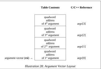
Illustration 28: Argument Vector Layout...242

Illustration 29: Privilege Levels...291

(14)

(15)

1.0 Introduction

The purpose of this text is to provide a reference for University level assembly language and systems programming courses. Specifically, this text addresses the x86-641 instruction set for the popular x86-64 class of processors using the Ubuntu 64-bit Operating System (OS). While the provided code and various examples should work under any Linux-based 64-bit OS, they have only been tested under Ubuntu 14.04 LTS (64-bit).

The x86-64 is a Complex Instruction Set Computing (CISC2_{) CPU design. This refers} to the internal processor design philosophy. CISC processors typically include a wide variety of instructions (sometimes overlapping), varying instructions sizes, and a wide range of addressing modes. The term was retroactively coined in contrast to Reduced Instruction Set Computer (RISC3_).

1.1 Prerequisites

It must be noted that the text is not geared toward learning how to program. It is assumed that the reader has already become proficient in a high-level programming language. Specifically, the text is generally geared toward a compiled, C-based high-level language such as C, C++, or Java. Many of the explanations and examples assume the reader is already familiar with programming concepts such as declarations, arithmetic operations, control structures, iteration, function calls, functions, indirection (i.e., pointers), and variable scoping issues.

Additionally, the reader should be comfortable using a Linux-based operating system including using the command line. If the reader is new to Linux, the Additional References section has links to some useful documentation.

1 For more information, refer to: http://en.wikipedia.org/wiki/X86-64

2 For more information, refer to: http://en.wikipedia.org/wiki/Complex_instruction_set_computing

Chapter

1

If you give someone a program, you will

(16)

1.2 What is Assembly Language

The typical question asked by students is 'why learn assembly?'. Before addressing that question, let's clarify what exactly assembly language is.

Assembly language is machine specific. For example, code written for an x86-64 processor will not run on a different processor such as a RISC processor (popular in tablets and smart-phones).

Assembly language is a “low-level” language and provides the basic instructional interface to the computer processor. Assembly language is as close to the processor as you can get as a programmer. Programs written in a high-level language are translated into assembly language in order for the processor to execute the program. The high-level language is an abstraction between the language and the actual processor instructions. As such, the idea that “assembly is dead” is nonsense.

Assembly language gives you direct control of the system's resources. This involves setting processor registers, accessing memory locations, and interfacing with other hardware elements. This requires a significantly deeper understanding of exactly how the processor and memory work.

1.3 Why Learn Assembly Language

The goal of this text is to provide a comprehensive introduction to programming in assembly language. The reasons for learning assembly language are more about understanding how a computer works instead of developing large programs. Since assembly language is machine specific, the lack of portability is very limiting for programming projects.

The process of actually learning assembly language involves writing non-trivial programs to perform specific low-level actions including arithmetic operations, function calls, using stack-dynamic local variables, and operating system interaction for activities such as input/output. Just looking at small assembly language programs will not be enough.

In the long run, learning the underlying principles, including assembly language, is what makes the difference between a coding technician unable to cope with changing languages and a computer scientist who is able to adapt to the ever-changing technologies.

(17)

1.3.1 Gain a Better Understanding of Architecture Issues

Learning and spending some time working at the assembly language level provides a richer understanding of the underlying computer architecture. This includes the basic instruction set, processor registers, memory addressing, hardware interfacing, and Input/ Output. Since ultimately all programs execute at this level, knowing the capabilities of assembly language provides useful insights into what is possible, what is easy, and what might be more difficult or slower.

1.3.2 Understanding the Tool Chain

The tool chain is the name for the process of taking code written by a human and converting it into something that the computer can directly execute. This includes the compiler, or assembler in our case, the linker, the loader, and the debugger. In reference to compiling, beginning programmers are told “just do this” with little explanation of the complexity involved in the process. Working at the low-level can help provide the basis for understanding and appreciating the details of the tool chain.

1.3.3 Improve Algorithm Development Skills

Working with assembly language and writing low-level programs helps programmers improve algorithm development skills by practicing with a language that requires more thought and more attention to detail. In the highly unlikely event that a program does not work the first time, debugging assembly language also provides practice debugging and requires a more nuanced approach since just adding a bunch of output statements is more difficult at the assembly language level. This typically involves a more comprehensive use of a debugger which is a useful skill for any programmer.

1.3.4 Improve Understanding of Functions/Procedures

(18)

1.3.5 Gain an Understanding of I/O Buffering

In a high-level language, input/output instructions and the associated buffering operations can appear magical. Working at the assembly language level and performing some low-level input/output operations provides a more detailed understanding of how input/output and buffering really works. This includes the differences between interactive input/output, file input/output, and the associated operating system services. 1.3.6 Understand Compiler Scope

Programming with assembly language, after having already learned a high-level language, helps ensure programmers understand the scope and capabilities of a compiler. Specifically, this means learning what the compiler does and does not do in relation to the computer architecture.

1.3.7 Introduction Multi-processing Concepts

This text will also provide a brief introduction to multi-processing concepts. The general concepts of distributed and multi-core programming are presented with the focus being placed on shared memory, threaded processing. It is the author’s belief that truly understanding the subtle issues associated with threading such as shared memory and race conditions is most easily understood at the low-level.

1.3.8 Introduction Interrupt Processing Concepts

The underlying fundamental mechanism in which modern multi-user computers work is based on interrupts. Working at a low-level is the best place to provide an introduction to the basic concepts associated with interrupt handling, interrupt service handles, and vector interrupts.

1.4 Additional References

Some key references for additional information are noted in the following sections. These references provide much more extensive and detailed information.

(19)

1.4.1 Ubuntu References

There is significant documentation available for the Ubuntu OS. The principal user guide is as follows:

◦ Ubuntu Community Wiki

◦ Getting Started with Ubuntu 1 6 .04

In addition, there are many other sites dedicated to providing help using Ubuntu (or other Linux-based OS's).

1.4.2 BASH Command Line References

BASH is the default shell for Ubuntu. The reader should be familiar with basic command line operations. Some additional references are as follows:

◦ Linux Command Line (on-line Tutorial and text)

◦ An Introduction to the Linux Command Shell For Beginners (pdf)

In addition, there are many other sites dedicated to providing information regarding the BASH command shell.

1.4.3 Architecture References

Some key references published by Intel provide a detailed technical description of the architecture and programming environment of Intel processors supporting IA-32 and Intel 64 Architectures.

◦ Intel® 64 and IA-32 Architectures Software Developer's Manual: Basic Architecture.

◦ Intel 64 and IA-32 Architectures Software Developer's Manual: Instruction Set

Reference.

◦ Intel 64 and IA-32 Architectures Software Developer's Manual: System Programming Guide.

If the embedded links do not work, an Internet search can help find the new location. 1.4.4 Tool Chain References

(20)

1.4.4.1 YASM References

The YASM assembler is an open source assembler commonly available on Linux-based systems. The YASM references are as follows:

◦ Yasm Web Site ◦ Yasm Documentation

Additional information regarding YASM may be available a number of assembly language sites and can be found through an Internet search.

1.4.4.2 DDD Debugger References

The DDD debugger is an open source debugger capable of supporting assembly language.

◦ DDD Web Site ◦ DDD Documentation

(21)

2.0 Architecture Overview

This chapter presents a basic, general overview of the x86-64 architecture. For a more detailed explanation, refer to the additional references noted in Chapter 1, Introduction.

2.1 Architecture Overview

The basic components of a computer include a Central Processing Unit (CPU), Primary Storage or Random Access Memory (RAM), Secondary Storage, Input/Output devices (e.g., screen, keyboard, mouse), and an interconnection referred to as the Bus.

A very basic diagram of the computer architecture is as follows:

Illustration 1: Computer Architecture

Chapter

2

Warning, keyboard not found. Press enter

to continue.

Screen / Keyboard /

Mouse Secondary Storage _{(i.e., SSD / Disk Drive /} Other Storage Media)

Primary Storage Random Access Memory (RAM) CPU

BUS

(22)

The architecture is typically referred to as the Von Neumann Architecture4_{, or the} Princeton architecture, and was described in 1945 by the mathematician and physicist John von Neumann.

Programs and data are typically stored on secondary storage (e.g., disk drive or solid state drive). When a program is executed, it must be copied from secondary storage into the primary storage or main memory (RAM). The CPU executes the program from primary storage or RAM.

Primary storage or main memory is also referred to as volatile memory since when power is removed, the information is not retained and thus lost. Secondary storage is referred to as non-volatile memory since the information is retained when powered off. For example, consider storing a term paper on secondary storage (i.e., disk). When the user starts to write or edit the term paper, it is copied from the secondary storage medium into primary storage (i.e., RAM or main memory). When done, the updated version is typically stored back to the secondary storage (i.e., disk). If you have ever lost power while editing a document (assuming no battery or uninterruptible power supply), losing the unsaved work will certainly clarify the difference between volatile and non-volatile memory.

2.2 Data Storage Sizes

The x86-64 architecture supports a specific set of data storage size elements, all based on powers of two. The supported storage sizes are as follows:

Storage Size (bits) Size (bytes)

Byte 8-bits 1 byte

Word 16-bits 2 bytes

Double-word 32-bits 4 bytes

Quadword 64-bits 8 bytes

Double quadword 128-bits 16 bytes

Lists or arrays (sets of memory) can be reserved in any of these types.

These storage sizes have a direct correlation to variable declarations in high-level languages (e.g., C, C++, Java, etc.).

(23)

For example, C/C++ declarations are mapped as follows:

C/C++ Declaration Storage Size (bits) Size (bytes)

char Byte 8-bits 1 byte

short Word 16-bits 2 bytes

int Double-word 32-bits 4 bytes

unsigned int Double-word 32-bits 4 bytes

long5 _Quadword _64-bits _{8 bytes}

long long Quadword 64-bits 8 bytes

char * Quadword 64-bits 8 bytes

int * Quadword 64-bits 8 bytes

float Double-word 32-bits 4 bytes

double Quadword 64-bits 8 bytes

The asterisk indicates an address variable. For example, int * means the address of an integer. Other high-level languages typically have similar mappings.

2.3 Central Processing Unit

The Central Processing Unit6_{(CPU) is typically referred to as the “brains” of the} computer since that is where the actual calculations are performed. The CPU is housed in a single chip, sometimes called a processor, chip, or die7_{. The cover image shows one} such CPU.

The CPU chip includes a number of functional units, including the Arithmetic Logic Unit8_{(ALU) which is the part of the chip that actually performs the arithmetic and} logical calculations. In order to support the ALU, processor registers9_{and cache}10 memory are also included “on the die” (term for inside the chip). The CPU registers and cache memory are described in subsequent sections.

It should be noted that the internal design of a modern processor is quite complex. This section provides a very simplified, high-level view of some key functional units within a CPU. Refer to the footnotes or additional references for more information.

5 Note, the 'long' type declaration is compiler dependent. Type shown is for gcc and g++ compilers. 6 For more information, refer to: http://en.wikipedia.org/wiki/Central_processing_unit

(24)

2.3.1 CPU Registers

A CPU register, or just register, is a temporary storage or working location built into the CPU itself (separate from memory). Computations are typically performed by the CPU using registers.

2.3.1.1 General Purpose Registers (GPRs)

There are sixteen, 64-bit General Purpose Registers (GPRs). The GPRs are described in the following table. A GPR register can be accessed with all 64-bits or some portion or subset accessed.

64-bit register Lowest 32-bits

Lowest 16-bits

Lowest 8-bits

rax eax ax al

rbx ebx bx bl

rcx ecx cx cl

rdx edx dx dl

rsi esi si sil

rdi edi di dil

rbp ebp bp bpl

rsp esp sp spl

r8 r8d r8w r8b

r9 r9d r9w r9b

r10 r10d r10w r10b

r11 r11d r11w r11b

r12 r12d r12w r12b

r13 r13d r13w r13b

r14 r14d r14w r14b

r15 r15d r15w r15b

(25)

When using data element sizes less than 64-bits (i.e., 32-bit, 16-bit, or 8-bit), the lower portion of the register can be accessed by using a different register name as shown in the table.

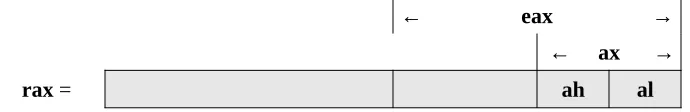
For example, when accessing the lower portions of the 64-bit rax register, the layout is as follows:

← eax → ← ax →

rax = ah al

As shown in the diagram, the first four registers, rax, rbx, rcx, and rdx also allow the bits 8-15 to be accessed with the ah, bh, ch, and dh register names. With the exception of ah, these are provided for legacy support and will not be used in this text.

The ability to access portions of the register means that, if the quadword rax register is set to 50,000,000,00010 (fifty billion), the rax register would contain the following value in hex.

rax = 0000 000B A43B 7400

If a subsequent operation sets the word ax register to 50,00010 (fifty thousand, which is C35016), the rax register would contain the following value in hex.

rax = 0000 000B A43B C350

In this case, when the lower 16-bit ax portion of the 64-bit rax register is set, the upper 48-bits are unaffected. Note the change in AX (from 740016 to C35016).

If a subsequent operation sets the byte sized al register to 5010 (fifty, which is 3216), the

rax register would contain the following value in hex.

rax = 0000 000B A43B C332

When the lower 8-bit al portion of the 64-bit rax register is set, the upper 56-bits are unaffected. Note the change in AL (from 5016 to 3216).

[image:25.540.110.455.119.175.2]

(26)

2.3.1.2 Stack Pointer Register (RSP)

One of the CPU registers, rsp, is used to point to the current top of the stack. The rsp register should not be used for data or other uses. Additional information regarding the stack and stack operations is provided in Chapter 9, Process Stack.

2.3.1.3 Base Pointer Register (RBP)

One of the CPU registers, rbp, is used as a base pointer during function calls. The rbp register should not be used for data or other uses. Additional information regarding the functions and function calls is provided in Chapter 12, Functions.

2.3.1.4 Instruction Pointer Register (RIP)

In addition to the GPRs, there is a special register, rip, which is used by the CPU to point to the next instruction to be executed. Specifically, since the rip points to the next instruction, that means the instruction being pointed to by rip, and shown in the debugger, has not yet been executed. This is an important distinction which can be confusing when reviewing code in a debugger.

2.3.1.5 Flag Register (rFlags)

The flag register, rFlags, is used for status and CPU control information. The rFlag register is updated by the CPU after each instruction and not directly accessible by programs. This register stores status information about the instruction that was just executed. Of the 64-bits in the rFlag register, many are reserved for future use.

The following table shows some of the status bits in the flag register.

Name Symbol Bit Use

Carry CF 0 Used to indicate if the previous operation

resulted in a carry.

Parity PF 2 Used to indicate if the last byte has an even number of 1's (i.e., even parity).

Adjust AF 4 Used to support Binary Coded Decimal

operations.

Zero ZF 6 Used to indicate if the previous operation

(27)

Sign SF 7 Used to indicate if the result of the previous operation resulted in a 1 in the most significant bit (indicating negative in the context of signed data).

Direction DF 10 Used to specify the direction (increment or decrement) for some string operations. Overflow OF 11 Used to indicate if the previous operation

resulted in an overflow.

There are a number of additional bits not specified in this text. More information can be obtained from the additional references noted in Chapter 1, Introduction.

2.3.1.6 XMM Registers

There are a set of dedicated registers used to support 64-bit and 32-bit floating-point operations and Single Instruction Multiple Data (SIMD) instructions. The SIMD instructions allow a single instruction to be applied simultaneously to multiple data items. Used effectively, this can result in a significant performance increase. Typical applications include some graphics processing and digital signal processing.

The XMM registers as follows:

(28)

xmm13 xmm14 xmm15

Note, some of the more recent X86-64 processors support 256-bit XMM registers. This will not be an issue for the programs in this text.

Additionally, the XMM registers are used to support the Streaming SIMD Extensions (SSE). The SSE instructions are out of the scope of this text. More information can be obtained from the Intel references (as noted in Chapter 1, Introduction).

2.3.2 Cache Memory

Cache memory is a small subset of the primary storage or RAM located in the CPU chip. If a memory location is accessed, a copy of the value is placed in the cache. Subsequent accesses to that memory location that occur in quick succession are retrieved from the cache location (internal to the CPU chip). A memory read involves sending the address via the bus to the memory controller, which will obtain the value at the requested memory location, and send it back through the bus. Comparatively, if a value is in cache, it would be much faster to access that value.

(29)

A block diagram of a typical CPU chip configuration is as follows:

Current chip designs typically include an L1 cache per core and a shared L2 cache. Many of the newer CPU chips will have an additional L3 cache.

As can be noted from the diagram, all memory accesses travel through each level of cache. As such, there is a potential for multiple, duplicate copies of the value (CPU register, L1 cache, L2 cache, and main memory). This complication is managed by the CPU and is not something the programmer can change. Understanding the cache and associated performance gain is useful in understanding how a computer works.

2.4 Main Memory

Memory can be viewed as a series of bytes, one after another. That is, memory is byte addressable. This means each memory address holds one byte of information. To store a double-word, four bytes are required which use four memory addresses.

Additionally, architecture is little-endian. This means that the Least Significant Byte (LSB) is stored in the lowest memory address. The Most Significant Byte (MSB) is stored in the highest memory location.

Illustration 2: CPU Block Diagram

Core 0

L2 Cache

Core 1

L1 Cache L1 Cache

BUS

(30)

For a double-word (32-bits), the MSB and LSB are allocated as shown below.

31 30 29 28 27 26 25 24 23 22 21 20 19 18 17 16 15 14 13 12 11 10 9 8 7 6 5 4 3 2 1 0

MSB LSB

For example, assuming the value of, 5,000,00010 (004C4B4016), is to be placed in a double-word variable named var1.

For a little-endian architecture, the memory picture would be as follows:

Based on the little-endian architecture, the LSB is stored in the lowest memory address and the MSB is stored in the highest memory location.

variable name

value Address

(in hex)

? 0100100C

00 0100100B

4C 0100100A

4B 01001009

var1 → 40 01001008

? 01001007

(31)

2.5 Memory Layout

The general memory layout for a program is as shown:

The reserved section is not available to user programs. The text (or code) section is where the machine language11_{(i.e., the 1's and 0's that represent the code) is stored. The} data section is where the initialized data is stored. This includes declared variables that have been provided an initial value at assemble-time. The uninitialized data section, typically called BSS section, is where declared variables that have not been provided an initial value are stored. If accessed before being set, the value will not be meaningful. The heap is where dynamically allocated data will be stored (if requested). The stack starts in high memory and grows downward.

Later sections will provide additional detail for the text and data sections.

2.6 Memory Hierarchy

In order to fully understand the various different memory levels and associated usage, it is useful to review the memory hierarchy12_{. In general terms, faster memory is more} expensive and slower memory blocks are less expensive. The CPU registers are small, fast, and expensive. Secondary storage devices such as disk drives and Solid State

11 For more information, refer to: http://en.wikipedia.org/wiki/Machine_code

high memory stack

. . . heap

BSS – uninitialized data data

text (code)

low memory reserved

(32)

Drives (SSD's) are larger, slower, and less expensive. The overall goal is to balance performance with cost.

An overview of the memory hierarchy is as follows:

Where the top of the triangle represents the fastest, smallest, and most expensive memory. As we move down levels, the memory becomes slower, larger, and less expensive. The goal is to use an effective balance between the small, fast, expensive memory and the large, slower, and cheaper memory.

Illustration 5: Memory Hierarchy

CPU Registers

Cache

Primary Storage Main Memory (RAM)

Secondary Storage (disk drives, SSD's, etc.)

Tertiary Storage

(remote storage, optical, backups, etc.) Smaller, faster, and more

expensive

(33)

Some typical performance and size characteristics are as follows:

Memory Unit Example Size Typical Speed

Registers 16, 64-bit registers ~1 nanoseconds13

Cache Memory 4 - 8+ Megabytes14

(L1 and L2)

~5-60 nanoseconds

Primary Storage (i.e., main memory)

2 – 32+ Gigabytes15 _{~100-150 nanoseconds}

Secondary Storage (i.e., disk, SSD's, etc.)

500 Gigabytes – 4+ Terabytes16

~3-15 milliseconds17

Based on this table, a primary storage access at 100 nanoseconds (100 ´ 10-9) is 30,000 times faster than a secondary storage access, at 3 milliseconds (3 ´ 10-3).

The typical speeds improve over time (and these are already out of date). The key point is the relative difference between each memory unit is significant. This difference between the memory units applies even as newer, faster SSDs are being utilized.

2.7 Exercises

Below are some questions based on this chapter. 2.7.1 Quiz Questions

Below are some quiz questions.

1) Draw a picture of the Von Neumann Architecture.

2) What architecture component connects the memory to the CPU? 3) Where are programs stored when the computer is turned off? 4) Where must programs be located when they are executing? 5) How does cache memory help overall performance?

6) How many bytes does a C++ integer declared with the declaration int use? 7) On the Intel X86-64 architecture, how many bytes can be stored at each address?

(34)

8) Given the 32-bit hex 004C4B4016 what is the: 1. Least Significant Byte (LSB)

2. Most Significant Byte (MSB)

9) Given the 32-bit hex 004C4B4016, show the little-endian memory layout showing each byte in memory.

10) Draw a picture of the layout for the rax register. 11) How many bits does each of the following represent:

1. al 2. rcx 3. bx 4. edx 5. r11 6. r8b 7. sil 8. r14w

12) Which register points to the next instruction to be executed? 13) Which register points to the current top of the stack?

14) If al is set to 0516 and ax is set to 000716, eax is set to 0000002016, and rax is set to 000000000000000016, and show the final complete contents of the complete

rax register.

15) If the rax register is set to 81,985,529,216,486,89510 (123456789ABCDEF16), what are the contents of the following registers in hex?

(35)

3.0 Data Representation

Data representation refers to how information is stored within the computer. There is a specific method for storing integers which is different than storing floating-point values which is different than storing characters. This chapter presents a brief summary of the integer, floating-point, and ASCII representation schemes.

It is assumed the reader is already generally familiar with binary, decimal, and hex numbering systems.

It should be noted that if not specified, a number is in base-10. Additionally, a number preceded by 0x is a hex value. For example, 19 = 1910 = 1316 = 0x13.

3.1 Integer Representation

Representing integer numbers refers to how the computer stores or represents a number in memory. The computer represents numbers in binary (1's and 0's). However, the computer has a limited amount of space that can be used for each number or variable. This directly impacts the size, or range, of the number that can be represented. For example, a byte (8-bits) can be used to represent 28_{or 256 different numbers. Those} 256 different numbers can be unsigned (all positive) in which case we can represent any number between 0 and 255 (inclusive). If we choose signed (positive and negative values), then we can represent any number between -128 and +127 (inclusive).

If that range is not large enough to handle the intended values, a larger size must be used. For example, a word (16-bits) can be used to represent 216_{or 65,536 different} values, and a double-word (32-bits) can be used to represent 232_{or 4,294,967,296} different numbers. So, if you wanted to store a value of 100,000 then a double-word would be required.

Chapter

3

There are 10 types of people in the world;

(36)

As you may recall from C, C++, or Java, an integer declaration (e.g., int <variable>) is a single double-word which can be used to represent values between -231 (−2,147,483,648) and +231_{- 1 (+}_{2,147,483,647}_).

The following table shows the ranges associated with typical sizes:

Size Size Unsigned Range Signed Range Bytes (8-bits) 28 _{0 to 255} _{-128 to +127}

Words (16-bits) 216 _{0 to 65,535} _{−32,768 to +32,767}

Double-words (32-bits) 232 _{0 to 4,294,967,295} _{−2,147,483,648 to}

+2,147,483,647

Quadword 264 _{0 to}₂64_{- 1} _-(₂63_{) to}₂63_{- 1}

Double quadword 2128 _{0 to}₂128_{- 1} _-(₂127_{) to}₂127_{- 1}

In order to determine if a value can be represented, you will need to know the size of the storage element (byte, word, double-word, quadword, etc.) being used and if the values are signed or unsigned.

• For representing unsigned values within the range of a given storage size,

standard binary is used.

• For representing signed values within the range, two's complement is used.

Specifically, the two's complement encoding process applies to the values in the negative range. For values within the positive range, standard binary is used.

For example, the unsigned byte range can be represented using a number line as follows:

For example, the signed byte range can also be represented using a number line as follows:

The same concept applies to halfwords and words which have larger ranges.

255 0

(37)

Since unsigned values have a different, positive only, range than signed values, there is overlap between the values. This can be very confusing when examining variables in memory (with the debugger).

For example, when the unsigned and signed values are within the overlapping positive range (0 to +127):

• A signed byte representation of 1210 is 0x0C16

• An unsigned byte representation of -1210 is also 0x0C16

When the unsigned and signed values are outside the overlapping range: • A signed byte representation of -1510 is 0xF116

• An unsigned byte representation of 24110 is also 0xF116

This overlap can cause confusion unless the data types are clearly and correctly defined.

3.1.1 Two's Complement

The following describes how to find the two's complement representation for negative values (not positive values).

To take the two's complement of a number: 1. take the one's complement (negate) 2. add 1 (in binary)

The same process is used to encode a decimal value into two's complement and from two's complement back to decimal. The following sections provide some examples. 3.1.2 Byte Example

For example, to find the byte size (8bits), two's complement representation of 9 and -12.

9 (8+1) = 00001001 12 (8+4) = 00001100

Step 1 11110110 Step 1: 11110011

Step 2 11110111 11110100

-9 (in hex) = F7 -12 (in hex) = F4

(38)

3.1.3 Word Example

To find the word size (16-bits), two's complement representation of -18 and -40.

18 (16+2) = 0000000000010010 40 (32+8) = 0000000000101000

Step 1 1111111111101101 Step 1 1111111111010111

Step 2 1111111111101110 Step 2 1111111111011000

-18 (hex) = 0xFFEE -40 (hex) = 0xFFD8

Note, all bits for the given size, words in these examples, must be specified.

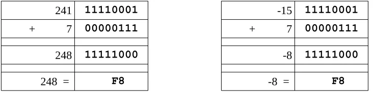
3.2 Unsigned and Signed Addition

As previously noted, the unsigned and signed representations may provide different interpretations for the final value being represented. However, the addition and subtraction operations are the same. For example:

241 11110001 -15 11110001

+ 7 00000111 + 7 00000111

248 11111000 -8 11111000

248 = F8 -8 = F8

The final result of 0xF8 may be interpreted as 248 for unsigned representation and -8 for a signed representation. Additionally, 0xF816 is the º (degree symbol) in the ASCII table.

As such, it is very important to have a clear definition of the sizes (byte, halfword, word, etc.) and types (signed, unsigned) of data for the operations being performed.

3.3 Floating-point Representation

[image:38.540.92.458.312.405.2]

(39)

3.3.1 IEEE 32-bit Representation

The IEEE 754 32-bit floating-point standard is defined as follows:

31 30 29 28 27 26 25 24 23 22 21 20 19 18 17 16 15 14 13 12 11 10 9 8 7 6 5 4 3 2 1 0

s biased exponent fraction

Where s is the sign (0 => positive and 1 => negative). More formally, this can be written as;

N = (−1)S × 1.F × 2E−127

When representing floating-point values, the first step is to convert floating-point value into binary. The following table provides a brief reminder of how binary handles fractional components:

23 ₂2 ₂1 ₂0 ₂-1 ₂-2 ₂-3

... 8 4 2 1 . 1/2 1/4 1/8 ...

0 0 0 0 . 0 0 0

For example, 100.1012 would be 4.62510. For repeating decimals, calculating the binary value can be time consuming. However, there is a limit since computers have finite storage sizes (32-bits in this example).

The next step is to show the value in normalized scientific notation in binary. This means that the number should have a single, non-zero leading digit to the left of the decimal point. For example, 8.12510 is 1000.0012 (or 1000.0012 x 20) and in binary normalized scientific notation that would be written as 1.000001 x 23_{(since the decimal} point was moved three places to the left). Of course, if the number was 0.12510 the binary would be 0.0012 (or 0.0012 x 20) and the normalized scientific notation would be 1.0 x 2-3_{(since the decimal point was moved three places to the right). The numbers} after the leading 1, not including the leading 1, are stored left-justified in the fraction portion of the double-word.

The next step is to calculate the biased exponent, which is the exponent from the normalized scientific notation plus the bias. The bias for the IEEE 754 32-bit floating-point standard is 12710. The result should be converted to a byte (8-bits) and stored in the biased exponent portion of the word.

(40)

3.3.1.1 IEEE 32-bit Representation Examples

This section presents several examples of encoding and decoding floating-point representation for reference.

3.3.1.1.1 Example → -7.7510

For example, to find the IEEE 754 32-bit floating-point representation for -7.7510:

Example 1: -7.75

• determine sign -7.75 => 1 (since negative) • convert to binary -7.75 = -0111.11₂ • normalized scientific notation = 1.1111 x 22 • compute biased exponent 2₁₀ + 127₁₀ = 129₁₀

◦ and convert to binary = 10000001₂ • write components in binary:

sign exponent mantissa

1 10000001 11110000000000000000000

• convert to hex (split into groups of 4)

11000000111110000000000000000000 1100 0000 1111 1000 0000 0000 0000 0000 C 0 F 8 0 0 0 0 • final result: C0F8 0000₁₆

3.3.1.1.2 Example → -0.12510

For example, to find the IEEE 754 32-bit floating-point representation for -0.12510:

Example 2: -0.125

• determine sign -0.125 => 1 (since negative) • convert to binary -0.125 = -0.001₂ • normalized scientific notation = 1.0 x 2-3 • compute biased exponent -3₁₀ + 127₁₀ = 124₁₀

◦ and convert to binary = 01111100₂ • write components in binary:

sign exponent mantissa

1 01111100 00000000000000000000000

• convert to hex (split into groups of 4)

(41)

3.3.1.1.3 Example → 4144000016

For example, given the IEEE 754 32-bit floating-point representation 4144000016 find the decimal value:

Example 3: 4144000016

• convert to binary

0100 0001 0100 0100 0000 0000 0000 00002 • split into components

0 10000010 100010000000000000000002

• determine exponent 10000010₂ = 130₁₀ ◦ and remove bias 130₁₀ - 127₁₀ = 3₁₀ • determine sign 0 => positive

• write result +1.10001 x 23 = +1100.01 = +12.25

3.3.2 IEEE 64-bit Representation

The IEEE 754 64-bit floating-point standard is defined as follows:

63 62 52 51 0

s biased exponent fraction

The representation process is the same, however the format allows for an 11-bit biased exponent (which support large and smaller values). The 11-bit biased exponent uses a bias of ±1023.

3.3.3 Not a Number (NaN)

When a value is interpreted as a floating-point value and it does not conform to the defined standard (either for 32-bit or 64-bit), then it cannot be used as a floating-point value. This might occur if an integer representation is treated as a floating-point representation or a floating-point arithmetic operation (add, subtract, multiply, or divide) results in a value that is too large or too small to be represented. The incorrect format or unrepresentable number is referred to as a NaN which is an abbreviation for not a number.

3.4 Characters and Strings

(42)

Computer memory is designed to store and retrieve numbers. Consequently, the symbols are represented by assigning numeric values to each symbol or character. 3.4.1 Character Representation

In a computer, a character19_{is a unit of information that corresponds to a symbol such as} a letter in the alphabet. Examples of characters include letters, numerical digits, common punctuation marks (such as "." or "!"), and whitespace. The general concept also includes control characters, which do not correspond to symbols in a particular language, but to other information used to process text. Examples of control characters include carriage return or tab.

3.4.1.1 American Standard Code for Information Interchange

Characters are represented using the American Standard Code for Information Interchange (ASCII20_{). Based on the ASCII table, each character and control character} is assigned a numeric value. When using ASCII, the character displayed is based on the assigned numeric value. This only works if everyone agrees on common values, which is the purpose of the ASCII table. For example, the letter “A” is defined as 6510 (0x41). The 0x41 is stored in computer memory, and when displayed to the console, the letter “A” is shown. Refer to Appendix A for the complete ASCII table.

Additionally, numeric symbols can be represented in ASCII. For example, “9” is represented as 5710 (0x39) in computer memory. The “9” can be displayed as output to the console. If sent to the console, the integer value 910 (0x09) would be interpreted as an ASCII value which in the case would be a tab.

It is very important to understand the difference between characters (such as “2”) and integers (such a 210). Characters can be displayed to the console, but cannot be used for calculations. Integers can be used for calculations, but cannot be displayed to the console (without changing the representation).

A character is typically stored in a byte (8-bits) of space. This works well since memory is byte addressable.

(43)

3.4.1.2 Unicode

It should be noted that Unicode21_{is a current standard that includes support for different} languages. The Unicode Standard provides series of different encoding schemes (UTF-8, UTF-16, UTF-32, etc.) in order to provide a unique number for every character, no matter what platform, device, application or language. In the most common encoding scheme, UTF-8, the ASCII English text looks exactly the same in UTF-8 as it did in ASCII. Additional bytes are used for other characters as needed. Details regarding Unicode representation are not addressed in this text.

3.4.2 String Representation

A string22_{is a series of ASCII characters, typically terminated with a NULL. The} NULL is a non-printable ASCII control character. Since it is not printable, it can be used to mark the end of a string.

For example, the string “Hello” would be represented as follows:

Character “H” “e” “l” “l” “o” NULL

ASCII Value (decimal) 72 101 108 108 111 0

ASCII Value (hex) 0x48 0x65 0x6C 0x6C 0x6F 0x0

A string may consist partially or completely of numeric symbols. For example, the string “19653” would be represented as follows:

Character “1” “9” “6” “5” “3” NULL

ASCII Value (decimal) 49 57 54 53 51 0

ASCII Value (hex) 0x31 0x39 0x36 0x35 0x33 0x0

Again, it is very important to understand the difference between the string “19653” (using 6 bytes) and the single integer 19,65310 (which can be stored in a single word which is 2 bytes).

3.5 Exercises

Below are some questions based on this chapter.

(44)

3.5.1 Quiz Questions Below are some quiz questions.

1) Provide the range for each of the following: 1. signed byte

2. unsigned byte 3. signed word 4. unsigned word 5. signed double-word 6. unsigned double-word

2) Provide the decimal values of the following binary numbers: 1. 00001012

2. 00010012 3. 00011012 4. 00101012

3) Provide the hex, byte size, two's complement values of the following decimal values. Note, two hex digits expected.

1. -310 2. +1110 3. -910 4. -2110

4) Provide the hex, word size, two's complement values of the following decimal values. Note, four hex digits expected.

(45)

5) Provide the hex, double-word size, two's complement values of the following decimal values. Note, eight hex digits expected.

1. -1110 2. -2710 3. +710 4. -26110

6) Provide the decimal values of the following hex, double-word sized, two's complement values.

1. FFFFFFFB16 2. FFFFFFEA16 3. FFFFFFF316 4. FFFFFFF816

7) Which of the following decimal values has an exact representation in binary? 1. 0.1

2. 0.2 3. 0.3 4. 0.4 5. 0.5

8) Provide the decimal representation of the following IEEE 32-bit floating-point values.

(46)

9) Provide hex, IEEE 32-bit point representation of the following floating-point values.

1. +11.2510 2. -17.12510 3. +21.87510 4. -0.7510

10) What is the ASCII code, in hex, for each of the following characters: 1. “A”

2. “a” 3. “0” 4. “8” 5. tab

11) What are the ASCII values, in hex, for each of the following strings: 1. “World”

(47)

4.0 Program Format

This chapter summarizes the formatting requirements for assembly language programs. The formatting requirements are specific to the yasm assembler. Other assemblers may be slightly different. A complete assembly language program is presented to demonstrate the appropriate program formatting.

A properly formatted assembly source file consists of several main parts; • Data section where initialized data is declared and defined. • BSS section where uninitialized data is declared.

• Text section where code is placed.

The following sections summarize the basic formatting requirements. Only the basic formatting and assembler syntax are presented. For additional information, refer to the yasm reference manual (as noted in Chapter 1, Introduction).

4.1 Comments

The semicolon (;) is used to note program comments. Comments (using the ;) may be placed anywhere, including after an instruction. Any characters after the ; are ignored by the assembler. This can be used to explain steps taken in the code or to comment out sections of code.

4.2 Numeric Values

Number values may be specified in decimal, hex, or octal.

When specifying hex, or base-16 values, they are preceded with a 0x. For example, to specify 127 as hex, it would be 0x7f.

When specifying octal, or-base-8 values, they are followed by a q. For example,

Chapter

4

I would love to change the world, but they

(48)

to specify 511 as octal, it would be 777q.

The default radix (base) is decimal, so no special notation is required for decimal (base-10) numbers.

4.3 Defining Constants

Constants are defined with equ. The general format is: <name> equ <value>

The value of a constant cannot be changed during program execution.

The constants are substituted for their defined values during the assembly process. As such, a constant is not assigned a memory location. This makes the constant more flexible since it is not assigned a specific type/size (byte, word, double-word, etc.). The values are subject to the range limitations of the intended use. For example, the following constant,

SIZE equ 10000

could be used as a word or a double-word, but not a byte.

4.4 Data Section

The initialized data must be declared in the "section .data" section. There must be a space after the word 'section'. All initialized variables and constants are placed in this section. Variable names must start with a letter, followed by letters or numbers, including some special characters (such as the underscore, "_"). Variable definitions must include the name, the data type, and the initial value for the variable.

The general format is:

<variableName> <dataType> <initialValue>

Refer to the following sections for a series of examples using various data types. The supported data types are as follows:

Declaration

(49)

dw 16-bit variable(s)

dd 32-bit variable(s)

dq 64-bit variable(s)

ddq 128-bit variable(s) → integer

dt 128-bit variable(s) → float

These are the primary assembler directives for initialized data declarations. Other directives are referenced in different sections.

Initialized arrays are defined with comma separated values. Some simple examples include:

bVar db 10 ; byte variable

cVar db "H" ; single character

strng db "Hello World" ; string

wVar dw 5000 ; word variable

dVar dd 50000 ; 32-bit variable

arr dd 100, 200, 300 ; 3 element array

flt1 dd 3.14159 ; 32-bit float

qVar dq 1000000000 ; 64-bit variable

The value specified must be able to fit in the specified data type. For example, if the value of a byte sized variables is defined as 500, it would generate an assembler error.

4.5 BSS Section

Uninitialized data is declared in the "section .bss" section. There must be a space after the word 'section'. All uninitialized variables are declared in this section. Variable names start with a letter followed by letters or numbers including some special characters (such as the underscore, "_"). Variable definitions must include the name, the data type, and the count.

The general format is:

<variableName> <resType> <count>

(50)

Declaration

resb 8-bit variable(s)

resw 16-bit variable(s)

resd 32-bit variable(s)

resq 64-bit variable(s)

resdq 128-bit variable(s)

These are the primary assembler directives for uninitialized data declarations. Other directives are referenced in different sections.

Some simple examples include:

bArr resb 10 ; 10 element byte array

wArr resw 50 ; 50 element word array

dArr resd 100 ; 100 element double array

qArr resq 200 ; 200 element quad array

The allocated array is not initialized to any specific value.

4.6 Text Section

The code is placed in the "section .text" section. There must be a space after the word 'section'. The instructions are specified one per line and each must be a valid instruction with the appropriate required operands.

The text section will include some headers or labels that define the initial program entry point. For example, assuming a basic program using the standard system linker, the following declarations must be included.

global _start _start:

(51)

4.7 Example Program

A very simple assembly language program is presented to demonstrate the appropriate program formatting.

; Simple example demonstrating basic program format and layout.

; Ed Jorgensen ; July 18, 2014

; ************************************************************ ; Some basic data declarations

section .data

;

---; Define constants

EXIT_SUCCESS equ 0 ; successful operation SYS_exit equ 60 ; call code for terminate

;

---; Byte (8-bit) variable declarations

bVar1 db 17 bVar2 db 9 bResult db 0

;

---; Word (16-bit) variable declarations

wVar1 dw 17000 wVar2 dw 9000 wResult dw 0

;

---; Double-word (32-bit) variable declarations

(52)

;

---; quadword (64-bit) variable declarations

qVar1 dq 170000000 qVar2 dq 90000000 qResult dq 0

; ************************************************************ ; Code Section

section .text global _start _start:

; Performs a series of very basic addition operations ; to demonstrate basic program format.

; ---; Byte example

; bResult = bVar1 + bVar2

mov al, byte [bVar1] add al, byte [bVar2] mov byte [bResult], al

; ---; Word example

; wResult = wVar1 + wVar2

mov ax, word [wVar1] add ax, word [wVar2] mov word [wResult], ax

;

---; Double-word example ; dResult = dVar1 + dVar2

(53)

;

---

x86-64 Assembly Language Programming with Ubuntu

Assembly Language

Table of Contents

Table of Contents

1.0 Introduction...1

2.0 Architecture Overview...7

3.0 Data Representation...21

4.0 Program Format...33

6.0 DDD Debugger...55

7.0 Instruction Set Overview...69

8.0 Addressing Modes...125

10.0 Program Development...151

12.0 Functions...167

13.0 System Services...191

14.0 Multiple Source Files...219

15.0 Stack Buffer Overflow...229

18.0 Floating-Point Instructions...257

19.0 Parallel Processing...279

21.0 Appendix A – ASCII Table...297

23.0 Appendix C – System Services...315

Table of Contents

Illustration Index

1.0 Introduction

Chapter

1.3 Why Learn Assembly Language

1.3.1 Gain a Better Understanding of Architecture Issues

1.3.4 Improve Understanding of Functions/Procedures

1.3.8 Introduction Interrupt Processing Concepts

1.4 Additional References

1.4.1 Ubuntu References

1.4.2 BASH Command Line References

1.4.3 Architecture References

1.4.4.1 YASM References

2.0 Architecture Overview

Chapter

2.2 Data Storage Sizes

Storage Size (bits) Size (bytes)

C/C++ Declaration Storage Size (bits) Size (bytes)

2.3 Central Processing Unit

2.3.1 CPU Registers

Lowest 16-bits

← eax → ← ax →

rax = 0000 000B A43B C350

2.3.1.2 Stack Pointer Register (RSP)

2.3.1.5 Flag Register (rFlags)

2.3.1.6 XMM Registers

2.3.2 Cache Memory

2.4 Main Memory

L2 Cache

MSB LSB

variable name

2.5 Memory Layout

BSS – uninitialized data data

CPU Registers

2.7 Exercises

3.0 Data Representation

Chapter

3.1.1 Two's Complement

3.1.3 Word Example

3.2 Unsigned and Signed Addition

3.3 Floating-point Representation

3.3.1 IEEE 32-bit Representation

3.3.1.1 IEEE 32-bit Representation Examples

3.3.1.1.2 Example → -0.12510

Example 3: 4144000016

3.3.3 Not a Number (NaN)

3.4 Characters and Strings

3.4.1.1 American Standard Code for Information Interchange

3.4.1.2 Unicode

3.5 Exercises

1. FFFFFFFB16 2. FFFFFFEA16 3. FFFFFFF316 4. FFFFFFF816

4.0 Program Format

4.1 Comments

Chapter

SIZE equ 10000

4.4 Data Section

<variableName> <dataType> <initialValue>

bVar db 10 ; byte variable

4.5 BSS Section

<variableName> <resType> <count>