Entropy and mutability for the q-states clock model in
small systems
Oscar A. Negrete1, Patricio Vargas1,∗,2 ID, Francisco J. Peña1,Gonzalo Saravia3, Eugenio E. Vogel2,3
1 Departamento de Física, Universidad Técnica Federico Santa María, Valparaíso, Chile;
2 Centro para el Desarrollo de la Nanociencia y la Nanotecnología, CEDENNA, Santiago, Chile
3 Departamento de Ciencias Físicas, Universidad de La Frontera, Temuco, Chile.
* Correspondence: [email protected]
Academic Editor: name
Version November 13, 2018 submitted to
Abstract:In this paper, we revisit the q-states clock model for small systems. We present results for the 1
thermodynamics of the q-states clock model fromq=2 toq=20 for small square latticesL×L, with 2
L ranging fromL=3 toL=64 with free-boundary conditions. Energy, specific heat, entropy and 3
magnetization are measured. We found that the Berezinskii-Kosterlitz-Thouless (BKT)-like transition 4
appears forq>5 regardless of lattice size, while the transition atq=5 is lost forL<10; forq≤4 5
the BKT transition is never present. We report the phase diagram in terms ofqshowing the transition 6
from the ferromagnetic (FM) to the paramagnetic (PM) phases at a critical temperature T1for small 7
systems which turns into a transition from the FM to the BKT phase for larger systems, while a second 8
phase transition between the BKT and the PM phases occurs at T2. We also show that the magnetic 9
phases are well characterized by the two dimensional (2D) distribution of the magnetization values. 10
We make use of this opportunity to do an information theory analysis of the time series obtained 11
from the Monte Carlo simulations. In particular, we calculate the phenomenological mutability and 12
diversity functions. Diversity characterizes the phase transitions, but the phases are less detectable as 13
qincreases. Free boundary conditions are used to better mimic the reality of small systems (far from 14
any thermodynamic limit). The role of size is discussed. 15
Keywords:q-states clock model; Entropy; Berezinskii-Kosterlitz-Thouless transition. 16
1. Introduction 17
The q-states clock model is the discrete version of the famous 2D XY model, which is probably the most extensively studied example showing the Berezinskii–Kosterlitz–Thouless (BKT) transition [1,2]. It is often used as a reference model due to its peculiar critical behaviour at the transition point and universal features [3–7]. Instead of the exclusion of an explicit continuous symmetry essential for the BKT transition, it can also emerge from a system without explicit continuous symmetry [7]. The Hamiltonian of the q-states clock model can be written in many forms, one of the simplest forms is the following expression, where no magnetic anisotropies and external magnetic field are included:
H=−J
∑
i<jcos(θi−θj), (1)
whereJ>0 is the ferromagnetic coupling connecting pairs of nearest neighboursiandj; the discrete 18
angle between the spin orientations is given byθi,j(η,q) =2πη/q, forη={0, 1, ..,q−1}. While the 19
exact XY model is recovered only in the limit of infiniteq, it has been found that the BKT characteristics 20
appear in the clock models whenq≥5 [8–11]. The nature of the phase transitions in the general clock 21
model has been widely studied with different theoretical and numerical approaches, which however 22
have given mixed results for the characterization of transitions at the lower bound ofq(for instance, 23
see the summary of the related debates in [12]). 24
In the present work, we want to consider the clock model as a generalization of the Ising model, 25
establishing the similarities and differences that arise due to the increase of the degrees of freedom due 26
to the local states at each site. All of this is always aimed at the behaviour of small systems, specifically, 27
we will focus on square lattices ranging from 3×3 up to 64×64. Free boundary conditions are preferred 28
since they better represent the importance of surface states in small systems. The clock clock model 29
systems under scrutiny will range fromq=2 (equivalent to the usual Ising model) toq=20. 30
There are various scattered results about the thermodynamics and phase transition of the clock 31
model. Therefore we report below a consistent compendium of its thermodynamic properties such 32
as internal energy,U, specific heat,C, entropyS, and magnetization. We also report the transition 33
temperatures,T1from the FM to thePphase for very smallqvalues continued as the transition from 34
the FM to the BKT phase for larger values ofq, andT2from the BKT phase to disordered paramagnetic 35
(P) phase. These series of results are elaborated into a phase diagramTCvsq, whereTCis determined 36
from theC(T)curves. 37
The information content of a sequence was measured in what was called mutability for the first 38
time by Vogel et al. [13] in a relationship with the characterization of the phase 2D transitions in 39
the Edward Andersen spin system as an alternative to the Binder cumulant analysis [14]. Later on, 40
an appropriate information recognizer was proposed (named wlzip) which optimizes recognition of 41
digital information associated to properties of the system [15]. The method was later successfully 42
applied to the reentrant phase diagram in the case of 3D Edwards-Anderson model. [16] Successive 43
applications of the information content methods dealt with stock markets [17], pension funds [18], 44
blood pressure [19], seismology [20], nematic transitions [21] and wind energy production [22]. 45
In the present paper, we follow the approach of the magnetic transitions [13,15] complemented 46
with the definitions of mutability and diversity [17] to be elaborated below. The aim is to have an 47
alternative way to characterize and distinguish the phases present in the q clock model. 48
In the next Section, we present the clock model and the main methods used to characterize 49
it. Presentation of results and discussion are given in Section 3, and the last Section is devoted to 50
conclusions. 51
2. Model and Methods 52
2.1. General Definitions 53
Let us begin by considering the q-states clock model on a two dimensional (2D) square lattice of dimensionsL×L=N, where the local magnetic moment or “spin”Siat siteican point in any of theq directions in a given plane.Siis then a 2D vector, i.e.Si= (cos(2qπk), sin(2qπk)), wherek=0, 1, ...q−1, with equal probability for allqvalues.Siare dimensionless vectors of magnitude one.
The isotropic Hamiltonian for such a system can be written as:
H=−J N
∑
i>jSi·Sj−B·
∑
iSi, (2)
whereJ>0 is the ferromagnetic exchange interaction to nearest neighbours; the sum extends to all 54
such pairs through the lattice, which is indicated by the symboli>junder the summation symbol. B 55
is an external field applied along one direction in the plane. 56
In this Hamiltonian, J is one unit of energy andBis also measured in energy units. This form is 57
2.2. Exact Theoretical Approach for a Small System 59
Let us begin by considering the theoretical approach for the q-states clock lattice withL = 3 introduced in the previous section. The partition function can be expressed as:
Z(T,B) =
λ
∑
n=1cne−En/T, (3)
where the coefficients cn is the number of all of the possible spin configurations compatible with 60
energyEnaccording to the Hamiltonian of Equation (2) ;λis the number of different energy levels. We 61
express energy and temperature in the same units, so the Boltzmann constant is set to the unity,kB=1. 62
The coefficients cn = c(En,q) for this small N = L×L = 3×3 lattice can be straightforwardly 63
calculated by using combinatorics; we show them in Table1forq=4 andq=6, and in Table2as 64
examples. For all evenqvalues (as the examples in Table1) some symmetry rules apply: energy 65
distribution is symmetric aroundEn =0, the majority of the density of states occurs forEn =0 and 66
c(−En,q) =c(En,q)holds. There areq9sates to be spread among all available energies in the energy 67
rangeEn= [−12, 12]. Due to symmetry,the total number of different energies areλ=11, 23, 47, 289 and 68
699 forq=2, 4, 6,8 and 10 respectively. 69
70
For odd q values the main symmetry of the Hamiltonian of Equation (2) for B = 0 is lost, 71
because spin inversionSi→ −Siis not possible . This is simply because, for oddqvalues, if there isSi 72
then−Sidoes not exist. Therefore the energy distribution and the corresponding degeneracy is not 73
symmetric aroundEn =0. Thus, the highest possible energy is not the negative value of the ground 74
state energy. However, as we will see, this symmetry lowering does not affect the thermodynamic 75
observables. 76
Once the partition function is known, the thermodynamic observables can be calculated directly. Thus for the cases of internal energyU, specific heatC, and entropyS, they can be obtained employing:
U(T) =T2 ∂
∂TlnZ(T,B), (4)
C(T) = ∂U
∂T , (5)
S(T) = U
Table 1.Coefficientsc(En,q)for a 3×3 lattice with free boundary conditions andB=0, forq=4 and
q=6. The first column enumerates energy levels,n, second and third columns give the corresponding energiesEand degeneraciesc(E, 4)respectively. Fourth and five columns show half of energies and degeneracies forq=6 respectively. The rest of the energies and degeneracies can be found using the following symmetry:c(−En, 6) =c(En, 6).
q = 4 q = 6
n En c(En, 4) En c(En, 6)
1 -12 4 -12 6
2 -10 32 -11 48
3 -9 128 -10.5 192
4 -8 248 -10 348
5 -7 896 -9.5 960
6 -6 2336 -9 2448
7 -5 4864 -8.5 2736
8 -4 10748 -8 5376
9 -3 19712 -7.5 11808
10 -2 29376 -7 14880
11 -1 39936 -6.5 22128
12 0 45584 -6 54072
13 1 39936 -5.5 54960
14 2 29376 -5 94032
15 3 19712 -4.5 175968
16 4 10748 -4 191514
17 5 4864 -3.5 231744
18 6 2336 -3 478752
19 7 896 -2.5 393360
20 8 248 -2 530892
21 9 128 -1.5 806736
22 10 32 -1 707760
23 12 4 -0.5 701712
24 0 1112830
Next table shows the results forq=5 where the energiesEnand degeneracies forn=1 ton=85 77
Table 2. Coefficientsc(En, 5)for a 3×3 lattice with free boundary conditions andB=0. In this case there are no symmetries and therefore we present allEnvalues with their respective degenerations, fromn=1 ton=85. Here, as explained in the manuscript the symmetrySi→ −Siis not present.
q = 5
n En c(En, 5) n En c(En, 5) n En c(En, 5) n En c(En, 5)
1 -12 5 23 -4.92705 15760 45 -1.57295 15760 67 2.30902 89000
2 -10.618 40 24 -4.76393 290 46 -1.47214 4100 68 2.47214 1340
3 -9.92705 160 25 -4.66312 6720 47 -1.30902 124320 69 2.73607 58080
4 -9.23607 290 26 -4.5 8960 48 -1.1459 1680 70 3 30200
5 -8.54508 800 27 -4.23607 30360 49 -1.04508 27920 71 3.16312 6720
6 -8.38197 40 28 -4.07295 680 50 -0.881966 57000 72 3.42705 64120
7 -8.11803 320 29 -3.97214 5280 51 -0.618034 117040 73 3.8541 21160 8 -7.8541 1680 30 -3.80902 23080 52 -0.454915 6958 74 4.11803 23640
9 -7.42705 680 31 -3.7082 410 53 -0.354102 9200 75 4.28115 1440
10 -7.16312 1600 32 -3.54508 29120 54 -0.190983 124320 76 4.54508 27920
11 -7 39936 33 -3.38197 5800 55 0 2 77 4.97214 5280
12 -6.73607 3040 34 -3.28115 1680 56 0.072949 64120 78 5.23607 17720 13 -6.57295 160 35 -3.11803 57000 57 0.236068 30360 79 5.66312 9880
14 -6.47214 1340 36 -2.95492 800 58 0.5 147600 80 6.09017 560
15 -6.30902 1760 37 -2.8541 21160 59 0.663119 1600 81 6.3541 9200
16 -6.04508 6960 38 -2.69098 23080 60 0.763932 17720 82 6.78115 1680 17 -5.88197 320 39 -2.59017 1240 61 0.927051 77360 83 7.47214 4100 18 -5.78115 1440 40 -2.42705 77360 62 1.19098 89000 84 8.59017 1240
19 -5.61803 5800 41 -2.26393 3040 63 1.3541 8440 85 9.70820 410
20 -5.3541 8440 42 -2.16312 9880 64 1.61803 117040
21 -5.19098 1760 43 -2 67600 65 1.88197 23640
22 -5.09017 560 44 -1.73607 58080 66 2.04508 29120
We invoke now the numeric simulations to calculate larger sizes for the same system. 79
2.3. Numerical Simulations 80
In addition to the theoretical calculations, most of the work will deal with numerical calculations 81
based on Monte Carlo (MC) simulations. A square latticeL×Lis chosen; free boundary conditions 82
are imposed; a site is randomly visited, and the energy cost,∆, of rotating the corresponding spin 83
aroundqpossible states is calculated: if the energy is lowered, the change of orientation is accepted; 84
otherwise, only when exp(−∆/T)≤r, the spin rotation is accepted, whereris a freshly-generated 85
random number in the range [0,1] with equal probability. This is the usual Metropolis algorithm. A 86
Monte Carlo step (MCS) is reached afterN=L×Lspin-rotation attempts. One of the main goals here 87
is to report the sensitive temperaturesT1andT2defining the transition from FM to BKT and from BKT 88
to PM (disordered) phase, for different systems. 89
For each lattice size and q value a sequence of temperatures was defined in the range [0.02,3] 90
at steps of 0.02 for each temperature, 5τMCSs are performed: the firstτMCS is used to equilibrate 91
at a fixed temperatureT, while the next 4τMCS is used to measure the observables every 20 MCSs, 92
reaching a total of 2×105=200, 000 measurements. Unless specified in a different wayτ=106in the 93
rest of the paper; thisτvalue gives stable results and leads to coincidence with the analytic expressions 94
obtained as described above. The energyU(T)is computed according to the Hamiltonian given by 95
Equation (2). With the internal energy known as a function ofTEquations (4), (5) and (6) can be used 96
to generate the thermodynamics. In parallel, the magnetizationM(T)for each temperature can also be 97
instantaneously measured. Alternatively, we can also use direct relationships based on the thermal 98
2.4. Thermal averages 100
The lattice average of the spin configuration, equivalent to the magnetization per siteM, is given by the following expression:
M= 1
N N
∑
j=1Sj , (7)
whereSjis the value of the spin at sitejat a given time,t, andN=L×L, is the total number of spins. In this particular caseMis a vector of two componentsM= (Mx,My). Normally, the magnitude or absolute value of this vector is calculated, i.e.|M| =qM2
x+My2. Then, the thermal average of the absolute value|M|, is<|M|>and it is given by
<|M|>= 1
Nc Nc
∑
i=1q
M2
x+M2y, (8)
whereNc=2×10⁵is the number of configurations used to perform thermal averages, as explained in the preceding section.
Energy is the main quantity used in the Monte Carlo method to reach thermal equilibrium. Therefore, afterτMCSs the internal energyUcan be obtained by averaging theNc=2 values forEk, wherek runs over the accepted configurations after the Metropolis algorithm, namely:
U=<E>= 1
Nc Nc
∑
k=1Ek, (9)
where every spin configuration is separated from the next one by 20MCs. The energy per site is then, 101
U/N, which is the thermal average of the lattice average of the system energy. 102
The specific heat is then calculated as proportional to the fluctuations of the energy as follows: 103
C= hE
2i − hEi2
T2 , (10)
C= 1
T2 1 Nc Nc
∑
k=1E2k
!
− 1
Nc Nc
∑
k=1Ek
!2
. (11)
The absolute entropyScan be calculated by calculating∆S(Tf,Ti) =S(Tf)−S(Ti)by numerical integration of the specific heat divided by the temperature, as follows:
∆S(Tf,Ti) =
Z Tf
Ti
C(T)
T dT. (12)
We know the entropy at zero temperature, because we know the energy degeneration atT=0. 104
For the caseB 6= 0, only one spin configuration has minimum energy (every spin aligned to B), 105
thereforeS(0) =0. On the other hand, when the magnetic field is zero, there areqferromagnetic spin 106
configurations with equal energies. Therefore,S(0) =lnq, hence thenS(T) =lnq+∆S(T, 0). 107
108
As we have seen, the thermal average of a physical quantity, is a summation overNcquantities 109
(normalized toNc), like the energies, magnetic moments, etc. However, the order of the sequence of 110
theseNcquantities is totally irrelevant in the result of this evaluation. Next we introduce the mutability 111
which is a quantity (defined in terms of information theory) that can be calculated from any temporal 112
sequence of quantities, like the energy, magnetic moment, etc. Mutability is a quantity that depends on 113
2.5. Information theory, mutability and diversity 115
Word length zipper (wlzip for short) is a compressor designed to recognize meaningful 116
information in a data chain. As its name tells it recognizes "words" of precise length and precise 117
location within the data chain. Then, it compresses less than other file compressors which precisely 118
optimize this function. In the case of wlzip the optimization is on the recognition of patterns beginning 119
at a precise location and for a given number of digits. In this way, physical properties and/or other 120
inherent properties of the system can be recognized. 121
The recognition of information within a file can render at least two parameters: mutability and 122
diversity. They were defined a few years ago including a working example given in Table 2 of Ref. [15] 123
Here we will very briefly review these definitions beginning with the basic rules under which wlzip 124
operates. Let us assume our data is contained in a vector file (one register per row) named "data.txt" 125
whose number of rows isλ(data)and its weight in bytes isw(data). We now create a map of previous 126
file in the following way: we go over each row of data.txt and whenever this value is new we add it as 127
a new row to a new file which will me named map.txt. So the process begins with the first element of 128
data.txt which is also the first element in map.txt. Then the second element of data.txt is considered: if 129
this element is new we add it as a second row in map.txt; if this element is the same as the previous 130
one one we just add a digit 1 to the right of this element in map.txt (1 here means one position from 131
last time this element appeared). The process continues like that so each time a new record is detected 132
a new row in map.txt is created, while repetitions are indicated as progressions of relative positions 133
to the right of the register in map.txt. At the end of the process, map.txt contains as many rows as 134
different values were present in data.txt; the more a value is repeated the wider the corresponding 135
row is in map.txt. In a sense this is like a histogram organized according to the appearance order. The 136
number of rows in data.txt isλ∗(map), while the weight of this file isw∗(map). 137
The mutabilityµ(data)of the entire file data.txt is simply given by
µ(data) = w
∗(data)
w(data) . (13)
Similarly, the diversity of the file data.txt is also a ratio, namely
δ(data) = λ
∗(data)
λ(data). (14)
Previous definitions can be also dynamic at the timetand considering theνrecords in data.txt counted from that one at timet. Then we can define the dynamic parameters associated to data.txt:
µ(t,ν) = w
∗(t,
ν)
w(t,ν) (15)
and
δ(t,ν) = λ
∗(t,
ν)
λ(t,ν) . (16)
As it was shown in the discussion accompanying Figure 1 of Ref. [17] referred to the Ising model, 138
mutability can be more appropriate to discuss variability of a parameter with changing conditions (like 139
increase of temperature) while diversity is more appropriate to discuss critical phenomena such as 140
phase transitions. This is one of the issues to be discussed below under the light of the results obtained 141
from the clock model. 142
3. Results and Discussions 143
Let us begin by considering the theoretical approach for the q-states clock model following 144
Equation (2) forB= 0, considering aL =3 lattice as it was presented in the previous section. We 145
thermodynamic quantities of the system can be analytically obtained as a function of the temperature 147
T. 148
Figure1shows the results obtained for internal energyU(T), specific heatC(T), and entropyS(T). 149
150
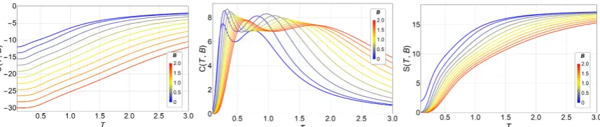
Figure 1.Internal Energy,U(left), Specific heat,C(middle), and Entropy,S(right), of the q-states clock model as a function of temperature,Tfor a 3×3 lattice, without magnetic field, for different values of
q. Fromq=2 (blue) toq=10 (red).
In the case of the specific heat,CvsT(center of Figure1) we see that the two peaks appear for 151
q≥6. Atq=5 we see only one peak, but notoriously more skewed to the right. We will see that this is 152
due to the small size of the lattice. Therefore for small systems, the BKT phase appears only forq≥6. 153
We can see here (Figure1right) the basic features of entropy in the low and high-temperature limits. 154
When no external field is applied, the energy ground state of the ferromagnetic q-states clock model 155
has a degeneracy equal toq, independent of the total number of spinsN, thereforeS(0) =lnq. On the 156
other hand, at very high temperatures, the exchange interaction is overridden, and every spin hasq 157
degrees of freedom with equal probabilities, hence the system degeneracy is equal toqN, and therefore 158
the entropyS(T>>J) =Nlnq, which is what it is observed in Figure2. 159
Figure2shows the same observables in the presence of magnetic fieldB, namely,U(T,B),C(T,B)
160
andS(T,B) for the caseq = 7 as an example; the shift of the transition temperatures due to the 161
variations of the magnetic field is clearly appreciated. This is also an exact analytical result obtained by 162
calculating straightforwardly the partition function of Equation (3). The magnetic field was applied 163
along the (1,0) direction, along which a possible spin orientation is always possible regardless of theq 164
value. 165
166
Figure 2.Internal Energy,U(T,B)(left), Specific heat,C(T,B)(middle), and Entropy,S(T,B)(right), of the q-states clock model (q=7) as a function of temperature,Tand field,B, for a 3×3 lattice. Different magnetic fields,B, are indicated by lines of different colors, fromB=0 (blue) toB=2(red).
ForB>0 the Zeeman term is added to the energy (see Equation (2)); therefore the FM ground 167
state energy is lowered by the external field. As an example forB=2, the Zeeman energy is -18, and 168
this is added to the ground state energy (-12) at zero field; therefore the new ground state energy is -30 169
(red curve in the left of Figure2. 170
We also observe that the specific heat,CvsTshapes maintain the two peaks, but they shift to higher 171
the external field favours ordered phases (FM and BKT) against disorder, and therefore the transition 173
temperatures increase with the strength of the external field. 174
The magnetic field breaks ergodicity, therefore atT = 0 there is only one ground state, thusS =0 175
forB 6= 0. However, at high temperatures the Zeeman term in Equation (2) is overridden and we 176
are back to the same situation as in previous analysis forB =0, namely, every spin hasqdegrees 177
of freedom with equal probabilities, hence the system degeneracy is equal toqN, and therefore the 178
entropyS(T>>J) =Nlnq, which is what it is observed in the right of Figure2. 179
180
3.1. MonteCarlo simulations 181
Next, we present and discuss the output from Monte Carlo simulations made for the q-states 182
clock model in lattices up to 64×64, with free boundary conditions. We began by simulating a 3×3 183
lattice for differentqvalues and comparing this numerical results to the analytic ones presented in 184
the previous section. We did not find a single difference, which is expected of course, but which also 185
serves as a check for the computer programs used extensively in the simulations reported next. Thus, 186
thermodynamic observables for lattices 10×10, 16×16, 32×32 and 64×64, are presented in figures 187
3 through 6 respectively. 188
189
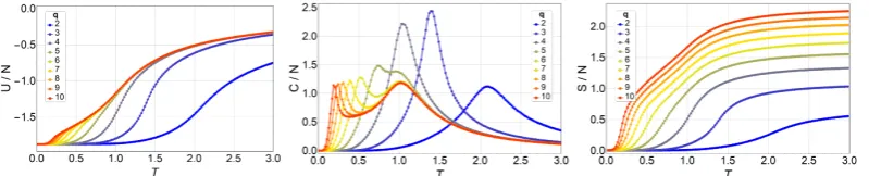
Figure 3. Internal Energy,U/N(left), Specific HeatC/N(middle) and EntropyS/N(right) of the q-states clock model as a function of temperature,Tfor aN=10×10 lattice, without magnetic field, forq=2 (blue) toq=10 (red).
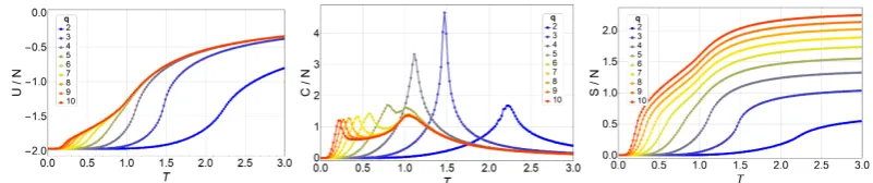
Figure 5. Internal Energy,U/N(left), Specific HeatC/N(middle) and EntropyS/N(right) of the q-states clock model as a function of temperature,Tfor aN=32×32 lattice, without magnetic field, forq=2 (blue) toq=10 (red).
Figure 6. Internal Energy,U/N(left), Specific HeatC/N(middle) and EntropyS/N(right) of the q-states clock model as a function of temperature,Tfor aN=64×64 lattice, without magnetic field, forq=2 (blue) toq=10 (red).
We observe an overall self-agreement in the shape of the EnergyU, Specific HeatC, and Entropy 190
S, as functions of temperature for the different lattices. The most noticeable change is the decrease in 191
temperature for the low-temperature peak in the specific heat curve as the size of the lattice increases. 192
For a given size, the peak of the specific heat occurs at a lower temperature asqincreases, and then 193
it splits in two peaks. Asqcontinues to increase, the high-temperature peak remains at the same 194
temperature whereas the low-temperature peak tends to lower temperatures (eventually to zero 195
temperature) asqincreases tending to infinity. This low-temperature peak,T1, is the transition from 196
the FM phase to the BKT like phase, which is characterized by vortex spin configurations and FM 197
spin-spin correlated configurations like waves. Both, vortex and spin waves are low energy excitation 198
that occurs asqincreases, therefore in theq→∞we expect thatT1→0. To be more specific about 199
the characterization of the clock model, we discuss next a phase diagram including the three possible 200
magnetic phases: FM (long-range order), BKT (short-range correlations) and PM (total disorder). 201
3.2. Phase diagram 202
In this section, we show the phase diagram for the clock model as extracted from the specific heat. 203
We collected the analytic results for the 3×3 lattice and the numerical results for the 10×10 and the 204
64×64 lattices. This is shown in Figure7forqranging from 2 to 20 by means of squares, triangles and 205
circles respectively. The texture and colour underneath illustrate the instantaneous magnetic phases for 206
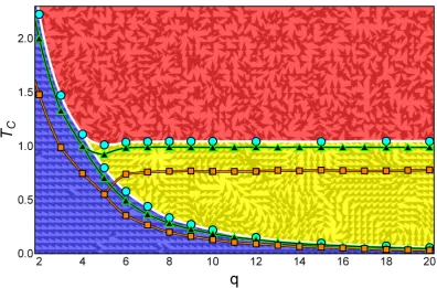
Figure 7. Phase diagram for the q-states clock model for a 3×3 lattice (squares), a 10×10 lattice (triangles) and a 64×64 lattice (circles) with free boundary conditions. For temperatures underT1the FM ordered phase dominates. Forq<5 the transition from this phase is to the disordered PM phase. For large enough lattices andq≥5 the transition from the FM phase is to the partially ordered BKT phase. Then, a transition at a higher temperatureT2appears separating the BKT phase from the PM phase; it can be noticed thatT2is essentially constant with respect toq. Background colors blue, yellow and red (from bottom to top) mark the FM, BKT and PM phases respectively. Spin orientations for one possible snapshot corresponding to the 64×64 lattice andq=9 are given in gray color over the background colors.
Several features in Figure7deserve special discussion. First, the lower critical temperatureT1 208
follows a monotonous decrease withqapproaching zero asymptotically. Second, the higher critical 209
temperatureT2keeps a constant value forq≥6. Third, forq=5 there is just one critical temperature 210
following the tendency ofT1, but forq = 10 (and also forq = 64) the two transitions are clearly 211
appreciated forq= 5. Fourth, an order parameter beyond the usual magnetization is necessary to 212
distinguish the BKT phase from the PM disordered phase. 213
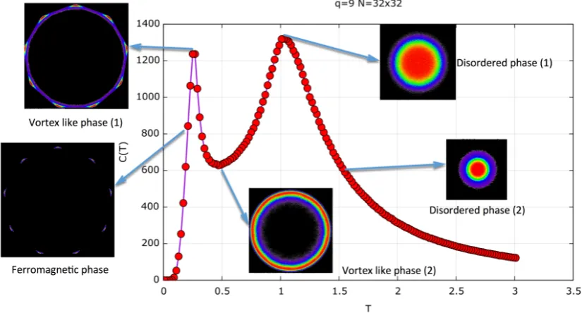
To be more specific about the different phases, Figure8shows the specific heat for a 32×32 lattice 214
as a function of temperature, where we show a two-dimensional (2D) order parameter, at certain 215
characteristic temperatures, which clearly discriminate the three (FM, BKT and PM) different phases. 216
The order parameter we use is the 2D distribution of the variableM= (Mcx,Myc), as defined in Eq. (7) , 217
the spin-lattice average at timetafter the thermalization process ofτMCSs. 218
This corresponds to the vector spin average for a given spin configuration at time,t. This vector is 219
then calculated after the thermalization, and every 20MCSs in a total ofNctimes. By plotting all 220
Ncvectors, we generate a 2D distribution that clearly characterizes the different phases. In the FM 221
phase, only certain directions of the spin are allowed, in the Figure8made forq=9 we see at low 222
temperature, that average magnetization vector points in nine directions which correspond to the 223
nine-fold symmetry of the FM states with equal probability. The BKT like phase is characterized 224
by spin waves and vortex structures; therefore the lattice average of the spin points to any of the 225
2πdirections but conserving in great extent its magnitude in every lattice average. Therefore a ring 226
structure is formed. In the disordered (PM) phase every spin in the lattice points randomly to any 227
decreasing magnitude as T increases; hence the circle begin to be filled with a higher probability (red 229
color) near the center. The color code goes from black (zero value), purple, blue, green, yellow and red 230
in increasing order of probability for this 2D order parameter. This parameter was already introduced 231
as a complex order parameter by Baek et al. [24] 232
Figure 8. Specific heat forq = 9 in a 32×32 lattice (red curve). The figures depict the 2D order parameter distribution ofM(two component vector), as defined in the text, forT=0.21, 0.27, 0.5, 1 and 1.51. In the ferromagnetic (FM) phase the distribution presents a nine-fold symmetry, indicating the 9 possible orientations of the magnetic domains in the FM phase at T=0.21. Vortex-like phase (1) shows (T=0.27) the onset of the BKT phase where we have smaller FM domains and vortex structures. This makes the thermal average magnetization (the 2D order parameter) to rotate but keeping its overall magnitude, at T=0.27 there is a reminiscence of the FM phase still present as can be seen in the ring structure with 9 maxima as observed atT=0.21. In T=0.5 a pure BKT phase is observed as a uniform ring structure but their radius begin to shrink, maintaining a smaller magnitude. AtT=1 is the onset of the disordered phase in which the magnitude of the magnetization decreases, filling the interior of the circle as a 2D Gaussian distribution with zero average, atT=1.51, the overall magnitude of the
Mparameter further shrinks. The color code of the 2D order parameter distribution goes from black, purple, blue, green, yellow and red as values of the 2D distribution increase. The radii of the ring-like 2D distributions represent the thermal magnetization modulus as a function of temperature, and this is given in Figure (10).
Next figure depicts snapshots of some spin configurations showing the spin arrangements that 233
.
Figure 9.Spin arrangements of the q-states clock model forq=9 in a 32×32 lattice. The figure depicts five snapshots each of one as a sample out of the 2×10⁵states used for thermal averages, at different temperatures. The temperatures are the same as shown in Figure8, i.e.T=0.21, 0.27, 0.5, 1 and 1.51. The snapshots clearly show the FM phase (a), the BKT like phase (b) and (c), and the disordered phase (d) and (e).
Next figure shows the magnetization modulus as the thermal average of the spin-lattice average, 235
as defined in Eq. (8) 236
Figure 10.Thermal average of the absolute value of the magnetization, as defined in Eq.(8) ( forq=2 (blue) toq=10(red) in a 32×32 lattice. The figure also depicts five starts forq=9 at the temperatures where the 2D order parameter are shown in Figure8, forT=0.21, 0.27, 0.5, 1 and 1.51. The values of their absolute magnetizations are the average radii of the ring and circular point distributions shown in Figure8.
Let us now consider the information content as an independent test to characterize these phase 237
transitions. We shall concentrate on the simulations for lattices 32×32 measuringµandδas defined 238
0.0 0.5 1.0 1.5 2.0 2.5 3.0
0.00 0.05 0.10 0.15 0.20 0.25 0.30
T
0.000 0.005 0.010 0.015 0.020
q=2
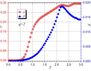
Figure 11.Mutability (µ) and diversity (δ) associated to the energy data forL=32,q=2.
Figure11presents the information content results for the same energy series generated by the 240
previously described MC algorithm; the case of a 32×32 lattice forq=2 is chosen for this report. The 241
open squares curve (red) gives the results for mutability, which presents a local maximum nearT=2.2 242
in agreement with the specific heat results (see Figure5). The solid circle’s curve (blue) is the result for 243
diversity showing a sharper absolute maximum atT=2.2. These are the results obtained from the 244
energy data; however, there are better parameters to register magnetic ordering whose consideration 245
is beyond the goals of the present paper [17]. At the moment we will stick to the energy data results 246
treated with diversity to directly compare with the energy curves, entropy and specific heat results 247
reported above. 248
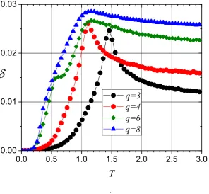
In Figure12we present the results forδin the cases forq = 3, q = 4, q = 6 andq = 8. The 249
ordinates have been multiplied by appropriate constants to fit in a common arbitrary scale since the 250
meaningful information is in the temperatures that are marked by each maximum or the inflections 251
of the curves. Forq=3 just one critical temperature is appreciated in agreement with the maximum 252
of the specific heat for this lattice size as shown in Figure5. A similar situation is observed forq=4 253
maximizing at lower temperatures around 1.1. Forq=6 a maximum around 1.1 and a "knee" just over 254
0.5 are visible in agreement with the two maxima for this value ofqreported in the figure for specific 255
heat. In the case ofq=8, the maximum near 1.1 is clearly present although a bit broader than for 256
q=6. The "knee" is barely appreciated as a tiny change of slope underT=0.5. 257
The results shown by previous two figures and similar ones for other intermediate values of 258
qshow that the information method is able to recognize the transitions present in the clock model 259
for low values ofqwhen this is applied to the energy data vectors produced by the MC simulations. 260
However, the phases are less detectable by this method asqincreases. Eventually, a different order 261
parameter more oriented to the magnetic states of the system rather than just the energy levels could 262
render better results. At the moment this is an open question, and it should be addressed in future 263
0.0 0.5 1.0 1.5 2.0 2.5 3.0 0.00
0.01 0.02 0.03
T
q=3
q=4
q=6
q=8
.
Figure 12.Diversityδassociated to the energy data forL=32,q=3,q=4,q=6 andq=8
4. Conclusions 265
Using analytically derived expressions and Monte Carlo simulations we explored the q-states 266
clock model for square lattices with free boundary conditions which better mimic the properties of 267
small systems to which this approach is intended. We calculated their thermodynamic properties 268
and characterized the three magnetic phases present for this model. The corresponding magnetic 269
phase diagram was calculated for lattices sizes up to 64×64. It turns out that there exists a FM 270
below a critical temperatureT1. Forq≥5 and lattice sizes over 10×10 a BKT-like phase appears for 271
temperatures betweenT1and a second critical temperatureT2separating this BKT phase from the 272
disordered paramagnetic phase. The BKT phase reflects partial magnetic ordering characterized by 273
vortex spin configurations and zones with FM spin-spin correlation, reflecting curling or wave-like 274
ordering. The three phases can be well characterized using the lattice spin average distribution. This 275
2D distribution shows characteristic patterns which clearly identify the three (FM, BKT and PM) 276
phases. 277
The entropy of the system always increases with temperature showing subtle slope changes at 278
the transition temperaturesT1andT2. The low-temperature limit for the entropy is simply given 279
by ln(q)in absence of magnetic field while it vanishes for any magnetic field that breaks ergodicity 280
yielding a singlet as a ground state. On the other hand, the high-temperature value for entropy tends 281
asymptotically toNln(q)thus reflecting that all degrees of freedom are equally probable. 282
The information theory method produces results in agreement with those of the specific heat of the 283
system. It distinguishes the phase diagram presented in Figure7for low values ofqthus confirming 284
previous results obtained by conventional treatments. However, this recognition is progressively lost 285
asqincreases. This is probably due to the fact that the information recognition pointed to the energy 286
values which are shared by more and more states asqincreases (contribution of the internal degrees of 287
freedom to the density of states). Eventually, different simulations involving a more elaborated order 288
both with vanishing magnetization. This work is in progress and should produce results in the near 290
future. 291
Acknowledgments:Francisco J. Peña acknowledges the financial support of FONDECYT-postdoctoral 3170010. P. 292
Vargas and E. Vogel acknowledge support from Financiamiento Basal para Centros Científicos y Tecnológicos 293
de Excelencia, under Project No. FB 0807 (Chile), P. Vargas acknowledges USM-DGIIP grant number PI-M-17-3 294
(Chile). E. Vogel acknowledges partial support from Fondecyt 1150019. 295
Author Contributions:P. Vargas and E. Vogel conceived the idea and formulated the theory. O. Negrete built the 296
computer program and edited the figures. G. Saravia wrote the mutability code. P. Vargas write the first version of 297
the manuscript, Francisco J. Peña contributed with discussions in the writing and edition of the same. All authors 298
have read and approved the final manuscript. 299
Conflicts of Interest:The authors declare no conflict of interest. 300
References 301
1. Berezinskii, V.L. Destruction of Long-range Order in One-dimensional and Two-dimensional Systems having 302
a Continuous Symmetry Group I. Classical Systems.Zh. Eksp. Teor. Fiz.1971,59, 907–920. 303
2. Kosterlitz, J.M.; Thouless, D.J. Long range order and metastability in two dimensional solids and superfluids. 304
(Application of dislocation theory).J. Phys. C Solid State Phys.1972,5, L124. 305
3. Kosterlitz, J.M.; Thouless, D.J. Ordering, metastability and phase transitions in two-dimensional systems. 306
J. Phys. C Solid State Phys.1973,6, 1181–1203. 307
4. Kosterlitz, J.M. The critical properties of the two-dimensional xy model.J. Phys. C Solid State Phys.1974,7, 308
1046–1060. 309
5. Jose, J.V.; Kadanoff, L.P.; Kirkpatrick, S.; Nelson, D.R. Renormalization, vortices, and symmetry-breaking 310
perturbations in the two-dimensional planar model.Phys. Rev. B1977,16, 1217–1241. 311
6. Kenna, R. The XY Model and the Berezinskii-Kosterlitz-Thouless Phase Transition.arXiv2005, arXiv:cond-312
mat/0512356. 313
7. 40 Years of Berezinskii-Kosterlitz-Thouless Theory; Jose, J.V., Ed; World Scientific: London, UK, 2013.
314
8. Elitzur, S.; Pearson, R.B.; Shigemitsu, J. Phase structure of discrete Abelian spin and gauge systems. 315
Phys. Rev. D1979,19, 3698–3714.
316
9. Cardy, J.L. General discrete planar models in two dimensions: Duality properties and phase diagrams. 317
J. Phys. A Math. Gen.1980,13, 1507–1515.
318
10. Fröhlich, J.; Spencer, T. The Kosterlitz-Thouless transition in two-dimensional Abelian spin systems and the 319
Coulomb gas.Commun. Math. Phys.1981,81, 527–602. 320
11. Ortiz, G.; Cobanera, E.; Nussinov, Z. Dualities and the phase diagram of the p-clock model.Nucl. Phys. B
321
2012,854, 780–814. 322
12. Borisenko, O.; Cortese, G.; Fiore, R.; Gravina, M.; Papa, A. Numerical study of the phase transitions in the 323
two-dimensional Z(5) vector model.Phys. Rev. E2011,83, 041120. 324
13. Vogel, E.E.; Saravia, G.; Bachmann, F.; Fierro, B.; Fischer, J. Phase transitions in Edwards-Anderson model by 325
means of information theory.Physica A2009,388, 4075–4082. 326
14. Binder, K. Finite size scaling analysis of ising model block distribution functions. Z. Phys. B1981,119, 327
119–140. 328
15. Vogel, E.E.; Saravia, G.; Cortez, L.V. Data compressor designed to improve recognition of magnetic phases. 329
Physica A2012,391, 1591–1601.
330
16. Cortez, L.V.; Saravia, G., Vogel, E.E. Phase diagram and reentrance for the 3D Edwards-Anderson model 331
using information theory.J. Magn. Magn. Mater.2014,372, 173–180. 332
17. Vogel, E.E.; Saravia, G. Information theory applied to econophysics: stock market behaviors.Eur. Phys. J. B
333
2014,2014, 4103. 334
18. Vogel, E.E.; Saravia, G; Astete, J.; Diaz, J.; Riadi, F. Information theory as a tool to improve individual 335
pensions: The Chilean case.Physica A424,2015, 372–382. 336
19. Contreras, D.J.; Vogel, E.E.; Saravia, G.; Stockins B. Derivation of a measure of systolic blood pressure 337
mutability: a novel information theory-based metric from ambulatory blood pressure tests.J. Amer. Soc.
338
Hypertension10,2016, 217-223.
20. Vogel, E.E.; Saravia, G; Pasten, D.; Munoz, V. Time-series analysis of earthquake sequences by means of 340
information recognizer.Tectonophysics712,2017, 723–728. 341
21. Vogel, E.E.; Saravia, G; Ramirez-Pastor, A.J. Phase diagrams in a system of long rods on two-dimensional 342
lattices by means of information theory.Phys. Rev. E96,2017, 062133. 343
22. Vogel, E.E.; Saravia, G; Kobe, S.; Schumann, R.; Schuster, R. A novel method to optimize electricity generation 344
from wind energy.Renewable Energy126,2018, 724–735. 345
23. Binder, K. Applications of Monte Carlo methods to statistical physics.Rep. Prog. Phys.1997,60, 487–559. 346
24. Seung Ki Baek, Petter Minnhagen and Beom Jun Kim, True and quasi-long-range order in the generalized 347