1
Evolutionary physical constants in Einstein’s field equations and the
redshift
Rajendra P. Gupta
Macronix Research Corporation, 9 Veery Lane, Ottawa, ON Canada K1J 8X4; [email protected]
Abstract We have shown that the use of evolutionary gravitational constants G, the speed of light
c, and cosmological constant Λ in the Einstein’s field equations leads to a very simple model that fits the supernovae Ia data with a single parameter as well as the standard ΛCDM model with two parameters, and has the predictive capability superior to the latter. We have shown that at the current time G and c both increase as dG/dt = 5.4GH0 and dc/dt = 1.8cH0 with H0 as the Hubble
constant, and Λ decreases as dΛ/dt = -1.2ΛH0. Negative finding on the variation of G with time
derived from the analysis of lunar laser ranging data in several studies has been attributed to the fact that these studies did not consider the variation of c simultaneously with G.
Keywords: cosmology: theory, cosmological parameters – galaxies: distances and redshifts – variable physical constants
1 INTRODUCTION
Varying physical constant theories have been in existence since time immemorial, especially since Dirac (1937, 1938) suggested such variation based on his large number hypothesis. The most comprehensive review of the subject was done by Uzan (2003) followed by his more recent review (Uzan 2011). Chiba (2011) has provided an update of the observational and experimental status of the constancy of physical constants. We therefore will not attempt to cover the subject’s current status except to mention a few of direct relevance to this work. Magueijo (2000, 2003) is a strong proponent of the variable speed of light theories. Accordingly, the model developed here will be considered generally Lorentz invariant which is true for any theory based on varying constants. We will be using the null results of Hofmann and Muller’s (2018) attempts to determine the variation of gravitational constant 𝐺 by analysing several decades of LLR data to establish that when the speed of light variation is included, one finds that 𝐺 and 𝑐 vary exactly in the proportion of 3 to 1.
We will follow Maharaj and Naidoo’s (1993) approach to include variable gravitational constant 𝐺 and cosmological constatnt Λ in the Einstein’s field equations, and generalize it to include the variable speed of light 𝑐, to obtain their solution for the Robert-Walker metric in Sec. 2. We will show that Λ̇/Λ = −1.2𝐻 and 𝐻̇/𝐻 = −0.6𝐻 where 𝐻 is the Hubble parameter. In Sec. 3 we will establish that 𝐺̇/𝐺 = 5.4𝐻 and
𝑐̇/𝑐 = 1.8𝐻. We will derive the expression for distance modulus 𝜇 vs. redshift 𝑧 in Sec. 4. Sec. 5 is devoted to state the methodology for fitting the supernovae Ia data (Scolnic et al. 2018) and apply the same to the new model and compare it with the fits obtained with the standard ΛCDM model. In the
final section, Sec. 6, we will discuss our findings and present conclusions.
The essence of this work is that the new model implicitly includes the cosmological constant (that is varying) and it can fit the supernovae Ia data with a single parameter almost as well as the ΛCDM model with two parameter, and it has the predictive capability superior to the latter. In addition, we not only establish that the physical constants vary, we provide exactly how much they vary.
2 EVOLUTIONARY CONSTANTS MODEL
We will develop our model in the general relativistic domain starting from the Robertson-Walker metric with the usual coordinates 𝑥𝜇 (𝑐𝑡, 𝑟, 𝜃, 𝜙):
𝑑𝑠2= 𝑐2𝑑𝑡2− 𝑎(𝑡)2[ 𝑑𝑟2 1−𝑘𝑟2+ 𝑟
2(𝑑𝜃2+ sin2𝜃𝑑𝜙2)].(1)
Here 𝑎(𝑡) is the scale factor and 𝑘 determines the spatial geometry of the universe: 𝑘 = −1 (closed), 0 (flat), +1 (open). The Einstein’s field equations may be written in terms of the Einstein tensor 𝐺𝜇𝜈, metric tensor 𝑔𝜇𝜈, and energy-momentum tensor 𝑇𝜇𝜈, as:
𝐺𝜇𝜈+ Λ𝑔𝜇𝜈= −8𝜋𝐺 𝑐4 𝑇
𝜇𝜈. (2)
When solved for the Robertson-Walker metric, we get the following non-trivial equations for the flat universe (𝑘 = 0) of interest to us here, with 𝑝 as the pressure and 𝜀 as the energy density:
2
𝑎̈𝑎+ 1 2(
𝑎̇ 𝑎)
2
= −4𝜋𝐺 𝑐2 𝑝 +
1
2Λ (3)
𝑎̇2 𝑎2=
8𝜋𝐺 3𝑐2𝜀 +
1
3Λ (4)
If we do not regard 𝐺, 𝑐 and Λ to be constant and define 𝐾 ≡ 𝐺/𝑐2, we may easily derive the continuity equation by taking time derivative of Eq. (4) and substituting in Eq. (3)
𝜀̇ +3𝑎̇
𝑎 (𝜀 + 𝑝) + 𝐾̇ 𝐾𝜀 +
Λ̇
8𝜋𝐾= 0. (5)
It reduces to the standard continuity equation when 𝐾 and Λ are held constant. And since the Einstein’s field equations require that the covariant derivative of the energy-momentum tensor 𝑇𝜇𝜈 be zero, we can interpret Equation (5) as comprising of two continuity equations (Maharaj & Naidoo 1993), viz
𝜀̇ +3𝑎̇
𝑎 (𝜀 + 𝑝) = 0, and (6)
8𝜋𝜀𝐾̇ + Λ̇ = 0. (7)
This separation simplifies the solution of the field equations (Eqs. 3 and 4). Eq. (6) yields the standard solution for the energy density 𝜀 = 𝜀0𝑎−3(1+𝑤). Here 𝑤 is the equation of state parameter defined as 𝑝 ≡ 𝑤𝜀 with 𝑤 = 0 for matter, 1/3 for radiation and −1 for Λ.
It has been explicitly discussed by Magueijo in several of his papers (e.g. Magueijo 2000) that this approach is not generally Lorentz invariant albeit relativistic. Moreover, one should ideally use Einstein-Hilbert action to obtain correct Einstein’s equations with variable 𝐺 and 𝑐. Our approach therefore may be considered quasi-phenomenological.
Since the universe expansion is determined by 𝐻(𝑡) ≡ 𝑎̇/𝑎, it is natural to assume the time dependence of any time dependent parameter to be proportional to 𝑎̇/𝑎 – the so called Machian scenario (Magueijo 2003). Let us therefore write
𝐾̇ 𝐾= 𝑘 (
𝑎̇ 𝑎),
Λ̇ Λ= 𝑙 (
𝑎̇ 𝑎) and
𝐻̇ 𝐻= 𝑚 (
𝑎̇
𝑎), i.e. (8)
𝐾 = 𝐾0𝑎𝑘, Λ = Λ0𝑎𝑙 and 𝐻 = 𝐻0𝑎𝑚. (9)
Here 𝑘 (not the same as in Eq. (1)) 𝑙 and 𝑚 are the proportionality constants, and subscript zero indicates the parameter value at current epoch (𝑡 = 𝑡0). With this substitution in Eq. (4) we may write
𝑎̇2
𝑎2= 𝐻02𝑎2𝑚= 8𝜋
3 (𝐾0𝑎 𝑘)𝜀
0𝑎−3(1+𝑤)+ 1 3Λ0𝑎
𝑙. (10)
Comparing the exponents of a of all the terms, we may write 2𝑚 = 𝑘 − 3 − 3𝑤 = 𝑙, and with 𝑤 = 0 for matter, we have 2𝑚 = 𝑘 − 3 = 𝑙. Thus, if we know 𝑘, we know 𝑙 and 𝑚. We can now have a closed analytical solution of Eq. (10) as follows (since 𝑎(𝑡0) ≡ 1):
𝑎(𝑡) = 𝑎(𝑡) 𝑎(𝑡0)= (
𝑡 𝑡0)
2 3+3𝑤−𝑘
; 𝑎̇ 𝑎=
2 3+3𝑤−𝑘𝑡
−1; (11)
𝑎̈ 𝑎̇= (
𝑎̇ 𝑎) (1 −
3+3𝑤−𝑘
2 ) ; and −𝑞 ≡ 𝑎̈𝑎 𝑎̇2=
−1−3𝑤+𝑘
2 . (12)
Here 𝑞 is deceleration parameter that does not depend on time, i.e. 𝑞0= 𝑞. As we know the radiation energy density is negligible at present, so we need be concerned with the matter only solutions, i.e. with 𝑤 = 0.
The deceleration parameter 𝑞0 has been analytically determined on the premise that expansion of the universe and the tired light phenomena are jointly responsible for the observed redshift, especially in the limit of very low redshift (Gupta 2018). One could see it as if the tired light effect is superimposed on the Einstein de Sitter’s matter only universe rather than the cosmological constant. By equating the expressions for the proper distance of the source of the redshift for the two, one gets 𝑞0= −0.4. Then from Eq. (12) we get 𝑘 = 1.8, and also 𝑙 = −1.2, and 𝑚 = −0.6. We thus have from Eq. (8) 𝐾̇/𝐾 = 1.8𝐻, Λ̇/Λ = −1.2𝐻 and 𝐻̇/𝐻 = −0.6𝐻.
3 VARYING G AND c FORMULATION
Having determined the value of 𝑘 = 1.8, and since the Hubble parameter is defined as 𝐻 = 𝑎̇/𝑎, we may write from Eqs. (8) and (9)
𝐾 = 𝐾0𝑎1.8, and 𝐾 𝐾
̇ = 1.8𝐻.
(13)
We may also write explicitly
𝐾̇ 𝐾=
𝐺̇ 𝐺−
2𝑐̇
𝑐 = 1.8𝐻. (14)
Taking 𝐻 at the current time as 𝐻0≃ 70 km s−1 Mpc-1 (2.27
× 10−18 s−1) we get 𝐾̇
𝐾= 4.09 × 10
−18 s−1= 1.29 ×
10−10 yr−1.
The findings from the Lunar Laser Ranging (LLR) data analysis provides the limits on the variation of 𝐺̇/𝐺 (7.1 ± 7.6 × 10⁻¹⁴) (Hofmann & Müller 2018), which is considered to be about three orders of magnitude lower than expected. However, the LLR data analysis is based on the assumption that the speed of light is constant and non-evolutionary. If this constraint is dropped then the finding would be very different.
As is well known (Merkowitz 2010), a time variation of 𝐺 should show up as an anomalous evolution of the orbital period 𝑃 of astronomical bodies expressed by Kepler’s 3rd law:
𝑃2=4𝜋2𝑟3
𝐺𝑀 , (15)
where 𝑟 is semi-major axis of the orbit, 𝐺 is the gravitational constant and 𝑀 is the mass of the bodies involved in the orbital motion considered. If we take time derivative of Eq. (15), divide by 𝑃2 and rearrange, we get
𝐺̇ 𝐺=
3𝑟̇ 𝑟 −
2𝑃̇ 𝑃 −
𝑀̇
𝑀 . (16)
If we write 𝑟 = 𝑐𝑡 then 𝑟̇ 𝑟=
1 𝑡+
𝑐̇
3
𝐺̇𝐺− 3𝑐̇
𝑐 = 3 𝑡−
2𝑃̇ 𝑃 −
𝑀̇
𝑀 . (17)
Since LLR measures the time of flight of the laser photons, it is the right hand side of Eq. (17) that is determined from LLR data analysis (Hofmann & Müller 2018) to be 7.1 ± 7.6 × 10⁻¹⁴ and not the right hand side of Eq. (16).
Then, taking the right hand side of Eq. (17) as 0 and combining it with Eq. (14), one can solve the two equations and get 𝐺̇/𝐺 = 5.4𝐻0= 3.9 × 10⁻¹⁰ yr−1 and 𝑐̇/𝑐 = 1.8𝐻0= 1.3 × 10⁻¹⁰ yr−1 . It should be emphasized that both 𝐺̇/𝐺 and 𝑐̇/𝑐 are positive and thus both of them are increasing with time rather than decreasing as is generally believed (Barnes & Dicke 1961, van Flandern 1975). This may be considered the most significant observational finding of cosmological consequences just by studying the Earth-Moon system.
4 REDSHIFT VS. DISTANCE MODULUS
The distance 𝑑 of a light emitting source in a distant galaxy is determined from the measurement of its bolometric flux 𝑓 and comparing it with a known luminosity 𝐿. The luminosity distance 𝑑𝐿 is defined as
𝑑𝐿= √ 𝐿
4𝜋𝑓 . (18)
In a flat universe the measured flux could be related to the luminosity 𝐿 with an inverse square relation 𝑓 = 𝐿/(4𝜋𝑑2). However, this relation needs to be modified to take into account the flux losses due to the expansion of the universe through the scale factor 𝑎, the redshift 𝑧, and all other phenomena which can result in the loss of flux. Generally accepted flux loss phenomena are as follows (Ryden 2017):
a. Increase in the wavelength causes the flux loss proportional to 1/(1 + 𝑧), and
b. In an expanding universe, an increase in detection time between two consecutive photons emitted from a source leads to a reduction of flux proportional to 𝑎, i.e. proportional to 1/(1 + 𝑧). Therefore, in an expanding universe the necessary flux correction required is proportional to 1/(1 + 𝑧)2. The measured bolometric flux 𝑓𝐵 and the luminosity distance 𝑑𝐿 may thus be written as:
𝑓𝐵= 𝐿/[4𝜋𝑑2(1 + 𝑧)2], and (19)
𝑑𝐿= 𝑑(1 + 𝑧). (20)
How does 𝑑 compare with and without varying 𝑐? Let us first consider the case of non-expanding universe. The distance from the point of emission at time 𝑡𝑒 to the point of observation at time 𝑡0 may be written as 𝑑𝑐 = ∫ 𝑐 𝑑𝑡
𝑡0
𝑡𝑒 . Therefore for constant
𝑐 = 𝑐0
𝑑𝑐0 = 𝑐0𝑡0(1 −
𝑡𝑒
𝑡0) (21)
When 𝑐 = 𝑐0𝑎1.8, and since 𝑎 = ( 𝑡 𝑡0)
2 1.2
from Eq. (11), we may
write
𝑑𝑐= 𝑐0∫ ( 𝑡 𝑡0)
3 𝑑𝑡 𝑡0
𝑡𝑒 =
𝑐0
𝑡03∫ 𝑡
3𝑑𝑡 𝑡0
𝑡𝑒 =
1
4𝑐0𝑡0(1 − 𝑡𝑒4
𝑡04). (22)
The ratio of the two distances may be considered the normalization factor 𝐹 when using the variable 𝑐 in calculating the proper distance of a source. Since 𝑎 ≡ 1/(1 + 𝑧), we may write for the source of redshift 𝑧 with emission time 𝑡𝑒
𝑡𝑒
𝑡0= 𝑎(𝑧)
0.6= (1 + 𝑧)−0.6 , and (23)
𝐹(𝑧) = 4[1 − (1 + 𝑧)−0.6]/[1 − (1 + 𝑧)−2.4] (24)
Now the proper distance of the source with variable 𝑐 may be defined as (Ryden 2017)
𝑑𝑃𝑐= ∫ (𝑡𝑡0 𝑎𝑐) 𝑑𝑡
𝑒 = ∫ (
𝑐0𝑎1.8 𝑎 ) 𝑑𝑡 𝑡0
𝑡𝑒 = 𝑐0∫ 𝑎
0.8 𝑑𝑡 𝑡0
𝑡𝑒
= 𝑐0∫ ( 𝑡 𝑡0)
4 3
𝑑𝑡 𝑡0
𝑡𝑒 =
3
7𝑐0𝑡0[1 − ( 𝑡𝑒
𝑡0) 7 3
]. (25)
From Eq. (11) 𝐻0≡ 𝑎̇/𝑎 = (2/1.2)𝑡0−1. Therefore,
𝑑𝑃𝑐= 1
1.4(𝑐0/𝐻0)[1 − (1 + 𝑧)
−1.4] . (26)
Thus the expression for 𝑑 to be substituted in Eq. (20) to determine the luminosity distance of the source is 𝑑 = 𝑑𝑃𝑐𝐹.
Since the observed quantity is distance modulus 𝜇 rather than the luminosity distance 𝑑𝐿, we will use the relation
𝜇 = 5 log(𝑑𝐿) + 25, (27)
= 5log (
1
1.4
𝑅
0(1 −
(1 + 𝑧
)−1.4)+ 5 log
(𝐹
(𝑧
))+5 log(1 + 𝑧) + 25. (28)
Here 𝑅0≡ 𝑐/𝐻0 and all the distances are in Mpc.
We will compare the new model, hereafter referred as VcGΛ (variable 𝑐, 𝐺 and Λ) model, with the standard ΛCDM model which is the most accepted model for explaining cosmological phenomena, and thus may be considered the reference models for all the other models. Ignoring the contribution of radiation density at the current epoch, we may write the distance modulus 𝜇 for redshift 𝑧 in a flat universe for the ΛCDM model as follows (Peebles 1993):
𝜇 = 5log [𝑅
0∫ 𝑑𝑢/√Ω
𝑚,0(1 + 𝑢)
3+ 1 − Ω
𝑚,0]
𝑧0
+5 log(1 + 𝑧) + 25. (29)
Here Ω0,𝑚 is the current matter density relative to critical density and 1 − Ω𝑚,0≡ ΩΛ,0 is the current dark energy density relative to critical density.
5 SUPERNOVAE Ia z-µ DATA FIT
We tried the VcGΛ model developed here to see how well it fits the best supernovae Ia data as compared to the standard ΛCDM model. The data fit is shown in Fig. 1. The VcGΛ model requires only one parameter to fit all the data (𝐻0= 68.90 ± 0.26 km 𝑠−1 Mpc−1) whereas the ΛCDM model requires two parameters (𝐻0= 70.16 ± 0.42 km 𝑠−1 Mpc−1 and Ω𝑚,0= 0.2854 ± 0.0245).
4
the two models, we divided the data in 6 subsets: a) 𝑧 < 0.5; b) 𝑧 < 1.0; c) 𝑧 < 1.5; d) 𝑧 > 0.5; and e) 𝑧 > 1.0; and f) 𝑧 > 1.5. In addition, we considered the fits for the whole data. The models were parameterized with subsets a), b) and c). The parameterized models were then tried to fit the data in the subsets that contained data with z values higher than in the parameterized subset. For example if the models were parameterized with data subset a) 𝑧 < 0.5, then the models were fitted with the data subsets d) 𝑧 > 0.5, e) 𝑧 > 1.0 and f) 𝑧 > 1.5.FIG. 1. Supernovae Ia redshift 𝑧 vs distance modulus µ data fit using the VcGΛ model as compared to the fit using the ΛCDM model.
The Matlab curve fitting tool was used to fit the data by minimizing 𝜒2 and the latter was used for determining the
corresponding 𝜒2 probability 𝑃 (Press et al. 1992). Here 𝜒2 is the weighted summed square of residual of 𝜇:
𝜒2= ∑ 𝑤
𝑖[𝜇(𝑧𝑖; 𝑅0, 𝑝1, 𝑝2… ) − 𝜇𝑜𝑏𝑠,𝑖] 2 𝑁
𝑖=1 , (30)
where 𝑁 is the number of data points, 𝑤𝑖 is the weight of the 𝑖th data point 𝜇𝑜𝑏𝑠,𝑖 determined from the measurement error 𝜎𝜇𝑂𝑏𝑠,𝑖 in the observed distance modulus 𝜇𝑜𝑏𝑠,𝑖 using the relation 𝑤𝑖= 1/𝜎𝜇2𝑂𝑏𝑠,𝑖, and 𝜇(𝑧𝑖; 𝑅0, 𝑝1, 𝑝2… ) is the model calculated distance modulus dependent on parameters 𝑅0 and all other model dependent parameter 𝑝1, 𝑝2, etc. As an example, for the ΛCDM models considered here 𝑝1≡ Ω𝑚,0 and there is no other unknown parameter.
We then quantified the goodness-of-fit of a model by calculating the 𝜒2 probability for a model whose 𝜒2 has been determined by fitting the observed data with known measurement error as above. This probability 𝑃 for a 𝜒2 distribution with 𝑛 degrees of freedom (DOF), the latter being the number of data points less the number of fitted parameters, is given by:
𝑃(𝜒2, 𝑛) = ( 1
Γ(𝑛2)) ∫ 𝑒
−𝑢𝑢𝑛2−1𝑑𝑢 ∞
𝜒2 2
, (31)
where Γ is the well know gamma function that is generalization of the factorial function to complex and non-integer numbers. Lower the value of 𝜒2 better is the fit, but the real test of the goodness-of-fit is the 𝜒2 probability 𝑃; higher the value of 𝑃 for a model, better is the model’s fit to the data. We used an online
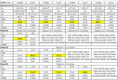
TABLE I. Parameterizing and prediction table for the two models. This table shows how well a model is able to fit the
data that is not used to determine the model parameters. The unit of R0 is Mpc and of H0 is km s-1 Mpc-1. P% is the χ2
probability in percent that is used to assess the best model for each category; higher the χ2 probability 𝑃 better is the model fit to the data. R2is the square of the correlation between the response values and the predicted response values. RMSE
is the root mean square error. Highest P% value in each category is shown in bold and the cell highlighted.
Action /Item ΛCDM VcGΛ ΛCDM VcGΛ ΛCDM VcGΛ ΛCDM VcGΛ
Parameterized
R0 4259±34 4337±18 4269±27 4351±17 4271±26 4352±17 4273±26 4351±16 Ωm,0 0.2601±0.0457 NA 0.2793±0.0261 NA 0.2818±0.0249 NA 0.2845±0.0245 NA H0 70.39±0.56 69.13±0.29 70.23±0.44 68.90±0.27 70.19±0.42 68.89±0.27 70.16±0.42 68.90±0.25
χ2 863.5 889.4 1018 1060 1033 1074 1036 1076
DOF 830 831 1023 1024 1040 1041 1046 1047
P% 20.39 7.83 53.82 21.15 55.53 23.26 58.11 26.02
R2
0.9961 0.9960 0.9969 0.9968 0.9970 0.9969 0.9970 0.9969
RMSE 1.020 1.035 0.9977 1.017 0.9965 1.016 0.9951 1.014
Model Fit
χ2 176.9 190
DOF
P% 97.59 89.84
R2 0.9605 0.9575 RMSE 0.905 0.938 Model Fit
χ2 19.54 17.01 17.59 16.75
DOF
P% 66.94 80.43 77.93 82.13
R2
0.8741 0.8904 0.8867 0.8921 RMSE 0.9216 0.86 0.8746 0.8533 Model Fit
χ2 4.090 1.946 3.167 1.983 3.076 1.986
DOF
P% 66.44 92.45 78.76 92.12 79.92 92.09
R2
0.5993 0.8093 0.6897 0.8057 0.6986 0.8054 RMSE 0.8256 0.5696 0.7265 0.5749 0.716 0.5754 NOT APPLICABLE SINCE THIS DATASET INCLUDES
THE DATASET USED TO PARAMETERIZE THE MODEL 23
6 NOT APPLICABLE SINCE
THIS DATASET INCLUDES THE DATASET USED TO PARAMETERIZE THE MODEL Dataset z>1.0; 23 points
Dataset z>1.5; 6 points
Model dataset all; 1048 points
Dataset z>0.5; 216 points
NOT APPLICABLE SINCE THIS DATASET INCLUDES
THE DATASET USED TO PARAMETERIZE THE MODEL
NOT APPLICABLE SINCE THIS DATASET INCLUDES
THE DATASET USED TO PARAMETERIZE THE MODEL NOT APPLICABLE SINCE
THIS DATASET INCLUDES THE DATASET USED TO PARAMETERIZE THE MODEL Model dataset z<0.5; 832 points Model dataset z<1.0; 1025 points Model dataset z<1.5; 1042 points
Dataset z>0.5; 216 points Dataset z>0.5; 216 points
NOT APPLICABLE SINCE THIS DATASET INCLUDES
THE DATASET USED TO PARAMETERIZE THE MODEL Dataset z>0.5; 216 points
5
calculator to determine 𝑃 from the input of 𝜒2 and DOF (Walker 2018). Our primary findings are presented in Table I. The unit of the Hubble distance 𝑅0 is Mpc and of the Hubble constant 𝐻0 is km s-1 Mpc-1. The table is divided in four categories vertically and four categories horizontally. Vertical division is based on the parameterizing data subset indicated in the second row and discussed above. The parameters determined for each model are in the first horizontal category. The remaining horizontal categories show the goodness-of-fit parameters for higher redshift subsets than used for parameterizing the models. Thus this table shows the relative predictive capability of the two models. The model cells with the highest probability in each category are shown in bold and highlighted.6 DISCUSSION AND CONCLUSION
As should be expected, the two parameter ΛCDM model is able to fit any data set better than the one parameter VcGΛ model. What is unexpected is that when parameterized with a relatively low redshift data the VcGΛ model is able to fit the higher redshift data better than the ΛCDM model. This shows that the second parameter in the latter, while trying to fit a limited dataset as best as possible, compromises the model fit for data not used for parameterizing. This means that the
ΛCDM model does not have as good a predictive capability (i.e. the capability to fit the data that is not included for determining the model parameters) as the VcGΛ model despite having twice as many parameters as the VcGΛ model. In addition the VcGΛ model has the analytical expression for the distance 𝜇 unlike the ΛCDM model which must be evaluated numerically.
One would notice that while 𝑅0 (and hence 𝐻0) values
are relatively stable with the parameterizing dataset containing higher and higher redshift values, varying no more than 0.35%, while the variation in the Ω𝑚,0 is up to 9.4%, i.e. 27 time higher. This confirms that Ω𝑚,0
parameter, and hence Λ through ΩΛ,0, is an artificially
introduced parameter to fit the data rather than being fundamental to the ΛCDM model. In contrast Λ is an integral part of the VcGΛ model. Since 𝐾 (≡ 𝐺/𝑐2) and Λ are related through Eq. (7), one could easily derive that the Λ term contributes 60% for the VcGΛ model against 70% for the ΛCDM model.
We have established that the supernovae 1a data is compatible with the variable constants proposition. This is contrary to the findings of Mould and Uddin (2014) who considered only the variation of 𝐺 in their work. We believe most of the negative findings on the variation of physical constants are possibly due to one considering the variation of a constant in isolation rather than
holistically for all the constants involved. We have established that the physical constants not only vary but also how much they vary: 𝑐̇/𝑐 = 1.8𝐻, 𝐺̇/𝐺 = 5.4𝐻,
Λ̇/Λ = −1.2𝐻 and 𝐻̇/𝐻 = −0.6𝐻. Also, from the null results on the variation of the fine structure constant (Gohar 2017, Rosenband et al. 2008) we can show that
ħ̇/ħ = 1.8𝐻. We urge that they be used in union rather than in isolation.
Acknowledgements Author is thankful to Franz Hofmann for providing his latest research paper and references on Lunar Laser Ranging. He is grateful to Dan Scolnic for providing the SNe Ia Pantheon data used in this work.
References
Barnes, C., Dicke, R. H. 1961 Phys. Rev. 124, 925. Chiba, T. 2011, Prog. Theor. Phys. 126, #6.
Dirac, P. A. M. 1937, Nature 139, 323.
Dirac, P. A. M. 1938, Proc. Roy. Soc. A 165, 199–208.
Gohar, H. 2017, Universe 3, 26.
Gupta, R. P. 2018, Int’l J. Astron. Astrophys. 8, 219; Universe 4, 104.
Hofmann, F, Müller, J. 2018, Class. Quant. Grav. 35, 035015.
Magueijo, J. 2000, Phys. Rev. D 62, 103521. Magueijo, J. 2003, Rept. Prog. Phys. 66, 2025.
Maharaj, S. D., Naidoo, R. 1993, Astrophys. Sp. Sci. 208, 261.
Merkowitz, S. M. 2010, Liv. Rev. Rel. 13, 7.
Mould, J., Uddin, S. A. 2014, PASA 31, e015.
Peebles, P. J. E. 1993, Principles of Physical Cosmology (Princeton University Press, N.J.).
Press, W. H., Teukolsky, S. A., Vetterling, W. T., Flannery, B. P. 1992, Numerical Recipes in C – The Art of Scientific Computing, 2nd Ed. (Cambridge University Press, U. K.).
Rosenband, T., Hume, D. B., Schmidt, P. O., Chou, C. W., Brusch, A., Lorini, et al. 2008, Science 319, 1808. Ryden, B. 2017 Introduction to Cosmology (Cambridge
University Press, U.K.).
Scolnic, D. M., Jones, D. O., Rest, A., et al. 2018, ApJ. 859, 101.
Uzan, J-P. 2003, Rev. Mod. Phys.75, 403. Uzan, J-P. 2011, Liv. Rev. Rel., 14, 2.
van Flandern, T. C. 1975, Mon. Not. Roy. Astron. Soc. 170, 333.