Article
Comparative Study of Clustering approaches Applied
to Spatial or Temporal Pattern Discovery.
Grassi Kelly1,2,3, Poisson-Caillault Émilie2,Bigand André2and Lefebvre Alain3* 1 WeatherForce, Toulouse, France ; [email protected]
2 LISIC EA 4491 Univ. Littoral, Calais, France ; [email protected]; [email protected] 3 IFREMER LER-BL Boulogne-sur-mer, France; [email protected]
* Correspondence: [email protected] † Current address: Affiliation 3
‡ These authors contributed equally to this work.
Abstract: Direct and hierarchical clustering approaches are compared to provide a first pattern discovery and times series segmentation. This unsupervised segmentation should be effective to help an expert labelling task. A divisive spectral clustering architecture with a no-cut criteria is proposed. This new algorithm achieves promise segmentation of spatial UCI databases and time series.
Keywords:Clustering, Pattern Discovery, Time series, Multi-Level Spectral Clustering.
0. Introduction
Pattern discovery in dataset is a fundamental task in various data mining applications. We investigate the way to detect spatial and/or temporal patterns without anya prioriknowledge about their number, shape or distribution. This unsupervised labelling should provide an optimal set of patterns to facilitate identification by a human expert. It will be considered optimal for the interpretation of a phenomenon if it covers all the existing structures within the data from dense to sparse, frequent to extreme. This labelled set is a crucial step to define a first training database to build a prediction system by learning machine techniques.
So, segmentation methods could be divided according to the cut processing way: by windows processing (time windows or space region] [? ? ], by generative models [? ? ], by either temporal/geometric cuts as breaking points [? ?] or clustering methods. The first two approaches need hypotheses about data distribution and pattern size. So, the outline of this paper is to compare the ability of the latter clustering methods so as to extract patterns in spatial and/or temporal cases.
Section 2 orders several clustering methods, and then focuses on our new adapted Multi-level Spectral Clustering (M-SC), combining spectral and hierarchical approaches. Section 3 presents experiment protocol to compare them in the task of pattern discovery and time series segmentation. Results on art. andin-situdata are discussed in Section 4. Their ability to label data is afterwards discussed with a focus on some supervised approaches.
1. Clustering approaches for pattern discovery
Many clustering approaches succeed in pattern segmentation in many applications as isolating object in picture background [?] or environmental event in marine multivariate time series [?]. In this case of time series segmentation, the temporal information are not included in the clustering process. These approaches could be distinguished according to their cut processing and their cut space: direct or hierarchical way, raw space from the data, or kernel or spectral space. The space choice refers to
data geometry. So, we propose viewpoint of direct and hierarchical methods and a new adapted M-SC.
Direct clustering. K-meansor K-Partitioning Around Medoids (PAM) algorithms are well employed to partition convex clusters with no overlap or for vector quantization (data reduction). They aim to partitionN observations into a fixed numberK of clusters, by minimizing the variance within each cluster. Density-Based Spatial Clustering (DBSCAN)approaches [? ] allow to relaxing the convexity constraint to dense cluster: (1) two points are agglomerated in the same cluster if they respect ae-distance and (2) the obtained cluster are saved if they have a minimal number of points (minPts). DBSCAN presents an interest for isolating noises; some observations will not be clustered. It could be a default for sparse cluster.Spectral clustering (SC)technique is used to separate clusters with low density. They require a point-to-point connexity within a cluster. SC is solved through a generalized problem of eigenvalues from a Laplacian matrixL.Lis computed from a similarity matrix Wissued from the data and a cut criterion. The clustering step is done in this spectral space from the K-first eigenvectors. There are many variants likespectral k-means (SC-Kmeans)that uses a standardized symmetric Laplacian matrix (LN JW = D−1/2WD1/2;Dthe degree matrix ofW) and K-means algorithm for partitioning [?] orspectral PAM (SC-PAM)that uses K-medoids algorithm.
Hierachical clustering. Conventional hierachical clustering (HC) techniques are based on the proximity between observations in the initial space. For the divisive ones, each observation is first assigned to its own cluster and then the algorithm proceeds iteratively, at each stage joining the two most similar clusters up to a single cluster. The partitioning trees differ from its proximity criterion; Ward.D2 is the most similar criterion of NJW one. An equivalent spectral approach was proposed by [? ], namedHierarchical-SC (H-SC), where the clustering step is based on HC with WARD.d2 criterion inLN JW eigenspace.Bipartite-SC (Bi-SC)[?] leads to a binary tree: at each level, each node is subdivised inK = 2 clusters according to the sign of the second eigenvector from the laplacian LShi=I−D−1/2WD1/2=I−LN JW. This constraint of separation in 2 groups are well adapted when a dominant structure is there (like background in an image).HDBSCANis a hierarchical extension of DBSCAN algorithm where a dissimilarity based one-neighborhood is used to aggregate observations.
For time-ordered observations, change-point analysis could be also added. We retain only approaches with clustering:Divisive estimation (e.divisive)andagglomerative estimation (e.agglo), which are also hierarchical approaches based on (e=)energy distance [?]. e.divisive defines segments through a binary bisection method and a permutation test. e.agglo creates homogeneous clusters based on an initial clustering. If no initial clustering are defined as such, each observation is assigned to its own segment.
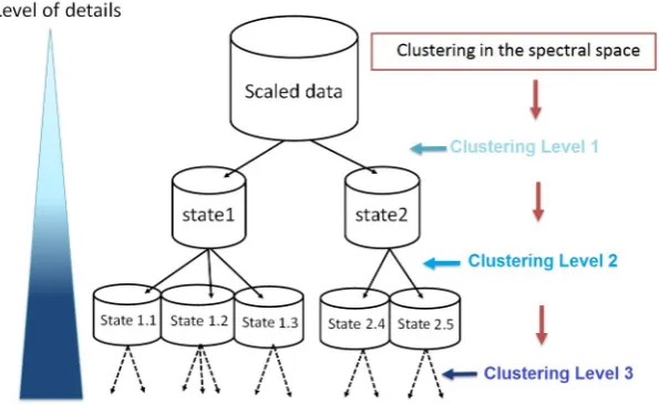
Figure 1.Multilevel Spectral Clustering scheme.
Figure 2.Multilevel Spectral Clustering scheme.
2. Comparison protocol
This work aims at comparing ability of the above methods to propose an effective clustering as first labelling. This section details labelled datasets, the tuning for each method should this step be required, and the list of performance metrics.
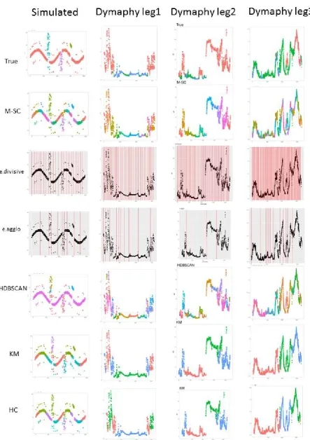
experimental dataset provided by DYPHYMA program [? ?], we used the Pocket Ferry Box data (PFB), coupled with the four algae concentrations from a multiple-fixed-wavelength spectral fluorometer (Algae Online Analyser [AOA], bbe Moldaenke).
Table 1. Dataset characteristics: name, area : exp.= experimental and art.= artificial, dimension (N observations×D features), number of classesC, distribution: the distribution percentage of the smallest class, (E) if equal. In bold: Time Series dataset.
Dataset Area Dimension C Distribution 1 Aggregate [?] art. 788×2 7 4.31 2 Compound [?
]
art. 399×2 6 4
3 Iris [?] exp. 150×4 3 33.33 (E) 4 Species [?] exp. 1, 600×64 100 1.6 (E)
5 Simulated[?] art. 1, 000×3 4 3.2
6 DYMAPHY
Leg1[?]
exp. 2, 032×18 3 12.20
7 DYMAPHY
Leg2[?]
exp. 3, 285×18 3 11.96
8 DYMAPHY
Leg3[?]
exp. 5, 599×18 3 7.30
Data processing and parameter tuning. Firstly, all dataset X are normalized to avoid impact of varying feature ranges in the clustering process. Zelnick and Perona locally adapted gaussian kernel with the 7thneighbors sigma distance in the similarity. For M-SC, min.points is therefore defined at 7. Direct spectral methods and M-SC and H-SC are based onLN JW Laplacian. So, all functions are computed with their default setting. But some parameters must be defined to choose the number of clusters (K).Kare fixed to the ground-truth class number for direct approaches, soK=C. Tree cut in the hierarchical methods (HC, H-SC) and level of divisive methods (Bi-SC, M-SC) are defined to obtain at leastCclusters and, sil.min is fixed at 0.7. For DBSCAN the determination ofK=Cclusters requirese-neighborhood. It is automatically determined by Unit Invariant Knee (UIK) estimation of the average k-nearest neighbor distance. For species dataset, the 20 principal components are retained to obtain a cumsum of 95% explained variance.
Comparison metrics. Two indicators are retained: (1) #Iso, the number of well-isolated patterns represented by more than half of the true positive observations; (2) the total accuracy, defined from the confusion table between theKclusters andCclasses after majority vote. Then three conventional unsupervised scores are added for interpretation: Adjusted Rand index, Dunn index, Silhouette score [?]. Here, they were computed in the raw space whatever the clustering methods used. Low Dunn index and averaged silhouette score from true label show the complexity to isolate each class, esp. for LEG sets, Dunn index computed from the ground-truth labels are around 10−4.
3. Clustering Results
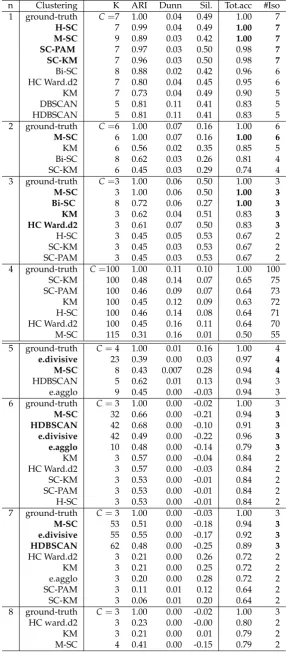
Table 2.Clustering approaches applied to pattern discovery, ordered by well-isolated pattern numbers (#Iso) with performance indicators: Adjusted Rand Index (ARI), Dunn and Silhouette (Sil.) indexes, total accuracy (Tot.acc) and the number of clustersK. (bold: #Iso=C, 0.00: non zero number). n is the dataset number.
n Clustering K ARI Dunn Sil. Tot.acc #Iso 1 ground-truth C=7 1.00 0.04 0.49 1.00 7
H-SC 7 0.99 0.04 0.49 1.00 7
M-SC 9 0.89 0.03 0.42 1.00 7
SC-PAM 7 0.97 0.03 0.50 0.98 7
SC-KM 7 0.96 0.03 0.50 0.98 7
Bi-SC 8 0.88 0.02 0.42 0.96 6
HC Ward.d2 7 0.80 0.04 0.45 0.95 6
KM 7 0.73 0.04 0.49 0.90 5
DBSCAN 5 0.81 0.11 0.41 0.83 5
HDBSCAN 5 0.81 0.11 0.41 0.83 5
2 ground-truth C=6 1.00 0.07 0.16 1.00 6
M-SC 6 1.00 0.07 0.16 1.00 6
KM 6 0.56 0.02 0.35 0.85 5
Bi-SC 8 0.62 0.03 0.26 0.81 4
SC-KM 6 0.45 0.03 0.29 0.74 4
3 ground-truth C=3 1.00 0.06 0.50 1.00 3
M-SC 3 1.00 0.06 0.50 1.00 3
Bi-SC 8 0.72 0.06 0.27 1.00 3
KM 3 0.62 0.04 0.51 0.83 3
HC Ward.d2 3 0.61 0.07 0.50 0.83 3
H-SC 3 0.45 0.05 0.53 0.67 2
SC-KM 3 0.45 0.03 0.53 0.67 2
SC-PAM 3 0.45 0.03 0.53 0.67 2
4 ground-truth C=100 1.00 0.11 0.10 1.00 100
SC-KM 100 0.48 0.14 0.07 0.65 75
SC-PAM 100 0.46 0.09 0.07 0.64 73
KM 100 0.45 0.12 0.09 0.63 72
H-SC 100 0.46 0.14 0.08 0.64 71
HC Ward.d2 100 0.45 0.16 0.11 0.64 70
M-SC 115 0.31 0.16 0.01 0.50 55
5 ground-truth C=4 1.00 0.01 0.16 1.00 4
e.divisive 23 0.39 0.00 0.03 0.97 4
M-SC 8 0.43 0.007 0.28 0.94 4
HDBSCAN 5 0.62 0.01 0.13 0.94 3
e.agglo 9 0.45 0.00 -0.03 0.94 3
6 ground-truth C=3 1.00 0.00 -0.02 1.00 3
M-SC 32 0.66 0.00 -0.21 0.94 3
HDBSCAN 42 0.68 0.00 -0.10 0.91 3
e.divisive 42 0.49 0.00 -0.22 0.96 3
e.agglo 10 0.48 0.00 -0.14 0.79 3
KM 3 0.57 0.00 -0.04 0.84 2
HC Ward.d2 3 0.57 0.00 -0.03 0.84 2
SC-KM 3 0.53 0.00 -0.01 0.84 2
SC-PAM 3 0.53 0.00 -0.01 0.84 2
H-SC 3 0.53 0.00 -0.01 0.84 2
7 ground-truth C=3 1.00 0.00 -0.03 1.00 3
M-SC 53 0.51 0.00 -0.18 0.94 3
e.divisive 55 0.55 0.00 -0.17 0.92 3
HDBSCAN 62 0.48 0.00 -0.25 0.89 3
HC Ward.d2 3 0.21 0.00 0.26 0.72 2
KM 3 0.21 0.00 0.25 0.72 2
e.agglo 3 0.20 0.00 0.28 0.72 2
SC-PAM 3 0.11 0.01 0.12 0.64 2
SC-KM 3 0.06 0.01 0.20 0.64 2
8 ground-truth C=3 1.00 0.00 -0.02 1.00 3
HC ward.d2 3 0.23 0.00 -0.00 0.80 2
KM 3 0.21 0.00 0.01 0.79 2
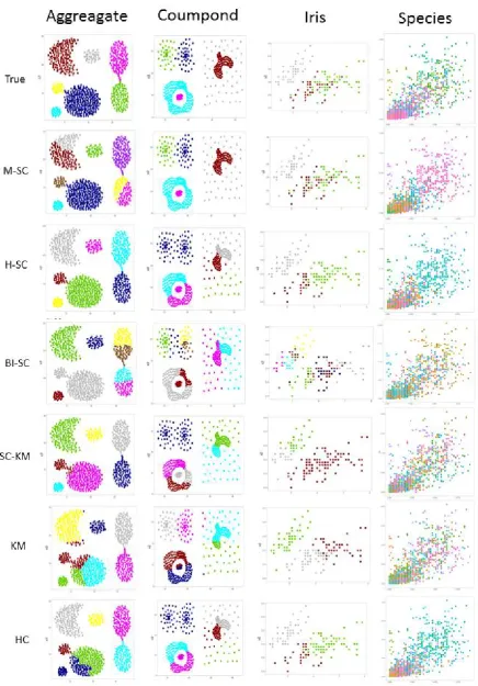
Spectral methods succeed in discovering all spatial patterns (#Iso=C) with high score for hierachical approaches: they could achieve 100% of accuracy, particularly M-SC except for species. It could be explained by the low class distribution and high connected clusters (averaged silhouette =0.1). For time series segmentation task, hierarchical methods better achieved to isolate event patterns, particularly M-SC, e.divisive and HDBSCAN. For LEG3, none of the algorithms isolate the 3 classes. M-SC succeeds to isolate them at level 3 withK=102 and a total accuracy of 93%. This number of clusters to label could appear too much, unreasonable for the human expert, but who can do more can do less.
4. Clustering for labeling
Clustering methods rely solely on data geometry to provide data segmentation. The purpose of this last part is to test their ability to provide a first labeling. So we compare them now with supervised techniques in the task of pattern discovery in time series.
Three basic machine solutions were explored: k-Nearest Neighbors classification (k-nn), Breiman’s Random Forest algorithm (RF, [?]) and a Multi-Layer percpetron (MLP). For the comparison, MLP was preferred to Time Delay Neural Networks to be fair with clustering approaches that do not taking account time parameter also.
Two training databases per dataset (from 5 to 8 in Table1) have been built. The first database represents 20% of the volume of each class in the table (80% for the test database) and the second 50%. Whatever the training and test base is, it covers allK=Ctemporal events. The attributes of an observation in the series are the classifier entries: for the 8th dataset, the input numberIis equal to 18. AndCis the output number for MLP and RF. For k-nn, two k values are chosen.kis set to 1 to assign the label of the closest observation and thenk=7 to obtain a a more unified segmentation (ie. with less than one class singleton among observations of other classes). MLP-1 here has one hidden layer whose neuron number is equal to(I+C)/2 and MLP-0 corresponds to linear perceptron (no hidden layer). Random Forest here consists of the vote of 500 trees withj√Ikvariables randomly sampled as candidates at each split.
The same unsupervised and supervised scores than in Table2are computed on the test databases and reported in Table3in order to compare clustering and classification approaches.
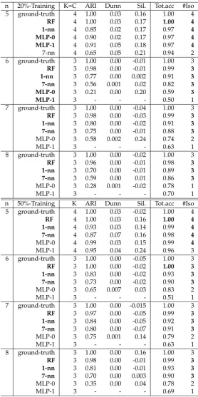
Learning techniques do not over-segment the time series due to the fixed number of their classes. RF and k-nn are able to isolate events with higher accucarcy and so low overlap between them for every dataset and every training cut. MLP-0 and MLP-1 are able to identify the 4 events of the simulated case but they are not efficient for in-situ cases (n=6-8) due to a lack of observations and unequal classes.
Divisive clustering techniques like M-SC does not suffer from unequal classes and has an easier way to detect events in the series. M-SC reached the same objective of well-isolated pattern number than supervised techniques like RF or knn. ARI and connectedness scores are highly dependent on the number of classes. In the supervised case, with a fixed K-number and computed from the test database only, ARI scores are higher than those of clustering approaches. However, the connectedness indices are not better.
Table 3. Classification approaches applied to pattern discovery, ordered by well-isolated pattern numbers (#Iso) with performance indicators for test database: Adjusted Rand Index (ARI), Dunn and Silhouette (Sil.) indexes, total accuracy (Tot.acc) and the number of clustersK. (bold: #Iso=C, 0.00: non zero number). n is the dataset number. RF= Random Forest, MLP-l= Multi-Layer Perceptron with l hidden layer, k-nn=k-nearest neighbors
n 20%-Training K=C ARI Dunn Sil. Tot.acc #Iso
5 ground-truth 4 1.00 0.03 0.16 1.00 4
RF 4 1.00 0.03 0.17 1.00 4
1-nn 4 0.85 0.02 0.17 0.97 4
MLP-0 4 0.90 0.02 0.17 0.97 4
MLP-1 4 0.91 0.05 0.18 0.97 4
7-nn 4 0.65 0.05 0.21 0.94 2
6 ground-truth 3 1.00 0.00 -0.01 1.00 3
RF 3 0.98 0.00 -0.01 0.99 3
1-nn 3 0.77 0.00 0.002 0.91 3
7-nn 3 0.56 0.001 0.02 0.82 3
MLP-0 3 0.21 0.00 0.20 0.59 3
MLP-1 3 - - - 0.50 1
7 ground-truth 3 1.00 0.00 -0.04 1.00 3
RF 3 0.98 0.00 -0.03 0.99 3
1-nn 3 0.80 0.00 -0.02 0.91 3
7-nn 3 0.75 0.00 -0.01 0.88 3
MLP-0 3 0.58 0.002 0.24 0.74 2
MLP-1 3 - - - 0.63 1
8 ground-truth 3 1.00 0.00 -0.02 1.00 3
RF 3 0.96 0.00 -0.01 0.98 3
1-nn 3 0.70 0.00 -0.01 0.89 3
7-nn 3 0.59 0.00 0.01 0.86 3
MLP-0 3 0.28 0.001 -0.02 0.78 1
MLP-1 3 - - - 0.70 1
n 50%-Training K ARI Dunn Sil. Tot.acc #Iso 5 ground-truth 4 1.00 0.03 -0.02 1.00 4
RF 4 1.00 0.03 0.16 1.00 4
1-nn 4 0.93 0.03 0.14 0.99 4
7-nn 4 0.87 0.07 0.16 0.98 4
MLP-0 4 0.99 0.03 0.15 0.99 4
MLP-1 4 0.95 0.04 0.24 0.96 3
6 ground-truth 3 1.00 0.00 -0.05 1.00 3
RF 3 1.00 0.00 -0.02 1.00 3
1-nn 3 0.83 0.00 -0.02 0.93 3
7-nn 3 0.73 0.00 -0.02 0.90 3
MLP-0 3 0.65 0.007 0.03 0.83 2
MLP-1 3 - - - 0.51 1
7 ground-truth 3 1.00 0.00 -0.015 1.00 3
RF 3 0.97 0.00 -0.05 0.99 3
1-nn 3 0.84 0.00 -0.05 0.92 3
7-nn 3 0.80 0.00 -0.07 0.91 3
MLP-0 3 0.75 0.001 0.14 0.79 2
MLP-1 3 - - - 0.63 1
8 ground-truth 3 1.00 0.00 0.16 1.00 3
RF 3 0.98 0.00 -0.01 0.99 3
1-nn 3 0.81 0.00 -0.01 0.93 3
7-nn 3 0.70 0.00 0.003 0.90 3
MLP-0 3 0.35 0.00 0.04 0.78 2
5. Conclusion
A relir car pas EUSIPCO mais ESSAN 2020
There is a large interest in representing high-resolution and high-dimension time series by optimized processing in order to extract relevant information for stakeholder. Huge potential for any application lies in the right combination of numerical methodology and representation without losing key-information as extreme events.
A Multilevel Spectral Clustering (M-SC) was proposed to segment multivariate time series in general patterns up to these extreme events by unsupervised way. On the basis of a simulated times series with high local connexity between events and global-shape signals, the proposed deep M-SC architecture give added value to segment all this shapes in contrast with related SC or hierarchical approach. First results obtained by M-SC on field MAREL Carnot time series are promising. Therefore, M-SC multilevel implicit segmentation will enable the implementation of nested approaches and to optimize extraction of knowledge when considering data covering different scales (temporal, frequency or spatial). We trust that the M-SC approach should be used for other marine applications (data from Ferry Box, gliders, . . . ) and also for other areas of application when dealing with the needs to segment data series and to identify general patterns and specific events without anya prioriknowledge.
Author Contributions:For research articles with several authors, a short paragraph specifying their individual contributions must be provided. The following statements should be used “Conceptualization, X.X. and Y.Y.; methodology, X.X.; software, X.X.; validation, X.X., Y.Y. and Z.Z.; formal analysis, X.X.; investigation, X.X.; resources, X.X.; data curation, X.X.; writing–original draft preparation, X.X.; writing–review and editing, X.X.; visualization, X.X.; supervision, X.X.; project administration, X.X.; funding acquisition, Y.Y. All authors have read and agreed to the published version of the manuscript.”, please turn to theCRediT taxonomyfor the term explanation. Authorship must be limited to those who have contributed substantially to the work reported.
Funding:
Acknowledgments:
Kelly Grassi’s PhD is funded by WeatherForce as part of its R & D program "Building an Initial State of the Atmosphere by Unconventional Data Aggregation".
MAREL-Carnot is part of the COAST-HF (Coastal ocean observing system - High frequency) network from the IR I-LICO (Infrastructure de Recherche LIttorale et COtière).
This project has received funding by JERICO-next from the European Union’s Horizon 2020 research and innovation program under grant agreement No 654410.
This work has been also partly financially supported by the European Union (ERDF), the French State, the French Region Hauts-de-France and Ifremer, in the framework of the project CPER MARCO 2015-2020.
Conflicts of Interest:Declare conflicts of interest or state “The authors declare no conflict of interest.” Authors must identify and declare any personal circumstances or interest that may be perceived as inappropriately influencing the representation or interpretation of reported research results. Any role of the funders in the design of the study; in the collection, analyses or interpretation of data; in the writing of the manuscript, or in the decision to publish the results must be declared in this section. If there is no role, please state “The funders had no role in the design of the study; in the collection, analyses, or interpretation of data; in the writing of the manuscript, or in the decision to publish the results”.
References
c