Multi Hop Routing Algorithm Using Spanning Tree for Network Lifetime in WSN

(1)

Multi-Hop Routing Algorithm Using Spanning Tree for

Network Lifetime in WSN

Deepthi M

1

Iswarya P

2

1

Department ofElectronic & Communication Engineering, SNS College of Engineering, Coimbatore

,

Tamil Nadu

, India

2_{Department of Computer Science &Engineering, SNS College of Engineering, Coimbatore, Tamil Nadu, India}

ABSTRACT

To balance the energy dissipation in the network and to provide long lifetime for network multiple paths in data gathering is used in wireless sensor network. The time where the base station from the sensors in the lifetime of the sensor, which are used in network lower lifetime and number of paths used to balance the energy will maximize the lifetime of the network when extra load is added to the specification node. To maximize the lifetime many existing protocols were used but here we use liner programming approach to solve. In this paper, we propose energy efficient spanning tree based on multi hop routing which will maximum the lifetime of network. The sequence of routing path is used to maximize the lifetime of the system, based on the location of the sensor node and base station. To maximize the lifetime of the network here an analysis in made.

Keywords: EESR PEDAPPA, PEDAP, CMLDA

I. INTRODUCTION

One of the fundamental problems in wireless sensor network is to maximize network lifetime. Most of the existing protocols take the cluster based approach or linear programming approach to solve the problem. In cluster based approach, the whole network is divided into groups where each group has a leader. The leader in a group is responsible to collect information from its member nodes and send data to base station or any nearest leader. In linear programming approach, the lifetime problem of WSN is formulated as maximum flow problem and solved using linear program.

As energy required in communication plays a major issue in energy depletion of the sensor node, we should minimize the number of transmissions along with efficient routing to achieve extended system lifetime. We consider a wireless sensor system where nodes are homogeneous and sensed data are highly correlated. A sensor network for continuous monitoring is a typical example of such a system. [2]

Mainly we have implemented the Data aggregation which used to reduce the data traffic which helps in

saving energy by combining multiple packets to single packet when sensed data are highly correlated.

In this paper, we propose a spanning tree based multi-hop routing technique to maximize network lifetime in terms of first node death. We assume that all nodes perform in-network data aggregation. Our proposed approach generates a transmission schedule which contains a collection of routing paths. A routing path forms a tree that spans all the sensor nodes. A transmission schedule denotes how data is collected from each sensor and propagated to base station. It represents a collection of routing paths that network will follow to maximize lifetime. We also show that our protocol generates a small transmission schedule which saves receiving energy.

II. METHODS AND MATERIAL

(2)

This protocol has a higher election overhead to update information among neighbours.

A maximum lifetime data gathering algorithm called MLDA, is proposed in the given location of each node and base station, MLDA gives the maximum lifetime of a network. MLDA works by solving a linear program to find edge capacities that flow maximum transmissions from each node to base station. The algorithm generates a schedule of multiple spanning trees that give maximum lifetime. MLDA gives almost near optimal lifetime of a network in terms of first node death. However, MLDA has an extreme run time complexity that requires solving linear program with O(n3) variables and constraints (n is the number of nodes in the network).

To overcome the limitation of MLDA, a cluster based heuristic algorithm called CMLDA is proposed in the CMLDA algorithm works by first clustering the nodes into groups of a given size. Each cluster’s energy is set to the sum of the energy of the contained nodes. The distance between clusters is set to the maximum distance between any pair of nodes of two clusters. After the cluster formation, MLDA is applied among the clusters to build cluster trees. CMLDA then utilizes energy balancing strategy within a cluster tree to maximize network lifetime.[2] CMLDA has a much faster running time than MLDA, but does not work well on networks that have nodes spaced far apart. CMLDA works better on dense network when nodes are deployed in groups in close proximity.

Tan and colleagues proposed two minimum spanning tree based data gathering and aggregation schemes to maximize the lifetime of the network, where one is the power aware version of the other. The non power aware version(PEDAP) extends the lifetime of the last node by minimizing the total energy consumed from the system in each data gathering round, while the power aware version (PEDAPPA) balance the energy consumption among nodes. In PEDAP, edge cost is computed as the sum of transmission and receiving energy. In PEDAPPA, an asymmetric communication cost is considered by dividing PEDAP edge cost with transmitter residual energy.

A node with higher edge cost is included later in the tree which results few incoming messages. Once the edge cost is established, routing information is

computed using Prim’s minimum spanning tree rooted at base station. The routing information is computed periodically after a fixed number of rounds (100). These algorithms assume all nodes perform in-aggregation and base station is aware of the location of the nodes. Notice that, the algorithm only considers sending node residual energy in edge cost function. In a densely deployed network, where receiving energy cost dominates over transmission energy cost, the protocol may fail to perform well.

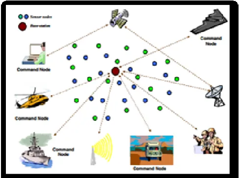
One of the advantages of wireless sensors networks (WSNs) is their ability to operate unattended in harsh environments in which contemporary human-in-the-loop monitoring schemes are risky, inefficient and sometimes infeasible. Therefore, sensors are expected to be deployed randomly in the area of interest by a relatively uncontrolled means,[1] e.g. dropped by a helicopter, and to collectively form a network in an ad-hoc manner. Given the vast area to be covered, the short lifespan of the battery-operated sensors and the possibility of having damaged nodes during deployment, large population of sensors are expected in most WSNs applications. It is envisioned that hundreds or even thousands of sensor nodes will be involved. Designing and operating such large size network would require scalable architectural and management strategies.

Figure 1. An articulation of sample WSN architecture for a military application

(3)

We use a first order radio model described in. In this model, energy required to run the transmitter or receiver circuitry is eelec = 50 nJ/bit and eamp = 100pJ/bit/m2 to run transmitter amplifier.[1] Energy required to transmit a data packet of size l bits from a node i to node j is given by the following equation.

Where dij is the distance between node i and j. Energy required to receive a l bit packet for any node j is given by

2. Maximum Life Time Routing

A. Problem Statement

Consider a network of n sensor nodes, with non-replenishable energy which are randomly placed in a network. Each node generates a fixed length data packet of size k bits and transmits to the base station. [2] All nodes in the network are capable of aggregating one or more incoming data packets with its own and send to base station or any other node.

Definition 1. In a data gathering round, each node generates a k-bit packet, possibly aggregates with others and transmits to base station or other node. In a data gathering round, base station receives sensed data of each sensor through aggregation, which reduces redundancy.[1]

Definition 2. Given the location of nodes, a routing tree specifies routing information of nodes such that sensed data from nodes reach to the base station. The routing tree spans all nodes in the network without any cycle. For a node, routing tree contains two pieces of information: to whom the node has to transmit data, and from which sensors it will receive data packet.[1]

Definition 3. A routing tree can be used for several rounds. We denote frequency to be the total number of rounds a routing tree will be used. [1]

Definition 4. We define schedule to be a collection of routing trees associated with their frequencies to

maximize the network lifetime. A schedule contains complete routing information for a WSN.[1]

Definition 5. Given a network of n sensor nodes s1, s2, ...sn, a routing tree T, we define the load of a sensor node si in routing tree T to be the energy required in receiving incoming packets and transmitting to next neighbor in a single round. We denote the load of a sensor node si by Loadi.[1]

B. Proposed Algorithm

In this section, we describe a greedy algorithm to generate routing trees for data gathering and aggregation. Given the location of nodes in the network, we are interested to compute a routing decision, which will maximize the lifetime of the network in terms of first node death. In other words, we want to keep all sensors operating as long as possible. [4] We assume that sensors are capable of aggregating any number of incoming data packets to a single data packet and transmitting to the base station or any other node when the sensed data are highly correlated.

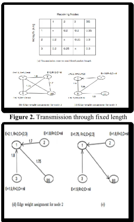
Figure 2. Transmission through fixed length

(4)

C. Edge Weight Assignment

Our routing tree generation algorithm starts with assigning link weight among nodes and forms a spanning tree. To transmit a k-bit packet from node i to node j the weight assignment is performed as follows:

where Ei is the current energy of the node i and Tij (k) is the energy required to transmit a k bit packet from node i to node j. The term Rj (k) denotes energy consumed to receive a k bit packet for node j. Notice that, the edge weight function is asymmetric which takes both the residual energy of sender node and receiver node under consideration. When a node sends a packet, it computes the edge weight for all its neighbors and selects the highest weighted edge to forward data towards base station. This avoids the receiving node to become overloaded by receiving too many incoming packets. Figure 1 shows an example of EESR weight assignment function. The variables E, R and C represent energy, root and child list of a node respectively. A lowest energy node is selected and its weight assignment is performed. Figure 1(a) denotes the transmission cost (Tij ) of each node for a fixed length packet. The received energy (Rj ) is assumed to be 0.1 unit for all nodes. Figure 1(b) illustrates the edge weight assignment for node 2, where weights are assigned by taking the minimum residual energy of sender and received node. In Figure 1(c), node 1 is selected as the parent of node 2, as this edge remains the highest residual energy both in sender and receiver. Next, node 3 is selected as the next lowest residual energy node. Figure 1(c) and 1(b) show the edge weight assignment and parent selection for node 3. Finally, in Figure 1(e), base station is selected as the parent of node 1. The detail of this weight assignment and parent selection is given in Figure 2 and 3

containing neighbour information for each node. It returns a sensor list A, containing routing information. We maintain a minpriority queue S to contain all nodes, which are yet to be connected to the routing tree.

The priority queue S is keyed by current energy level of nodes

E. Routing in Sensor Networks

A new class of spanning trees called Vertex Subset Degree Preserving Spanning Tree (A-DPST) is defined as a spanning tree T of the graph G(V,E) such that degT (vi) =deg G(vi) for all vi in A which is a nonempty subset of V[4]. The minimum spanning tree problem with an added constraint that the vertices of A should preserve their degrees in the spanning tree which can be termed as A-Degree Preserving Minimum Spanning Tree (A-DPMST).We are using an algorithm for multi-clustering in sensor networks using such A-DPMST is proposed.

The sensor network is considered as a graph whose vertices are the sensors along with the cluster heads, the base station, and the links between them as the edges. Now the collection of cluster heads say A is a nonempty subset of the vertex set of the graph and the construction of the routing tree for the sensor network becomes the problem of finding A-Degree Preserving Spanning Tree in the graph [2]. Because in the sensor network this A-DPST will be a minimally connected sub network in which all the links to the cluster heads are maintained. Since in the tree every other node is either directly connected to the head or having a path to the head, routing will be complete. Such routing could be made optimum by deploying higher energy node as the sensor heads of the clusters.

F. Selecting Routing Tree Frequency

(5)

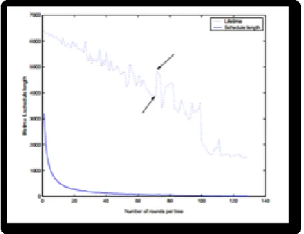
[3]Figure 4 shows the influence of tree frequency on network lifetime and schedule length on a 50x50m2 network consisting of 70 sensor nodes. The value in the x axis represents tree frequency of each tree in the schedule. The top curve represents the lifetime of the network using fixed tree frequency. The bottom curve depicts relation between tree frequency and schedule length. Although schedule length starts dropping with the increase of tree frequency, the relationship between tree frequency and network lifetime remains non linear. It could be anticipated that as we use each tree for higher number of rounds, both schedule length and lifetime would be reduced. Instead, our results show that network lifetime increases from 4000 to 5439 when the tree frequency is 70 and 72 respectively which proves our non linear claim between network lifetime and schedule length. It gives the indication that all trees should not be used for same number of rounds. Each tree should be assessed to find an appropriate tree frequency. As a result, there is a need for a dynamic tree frequency for each routing tree which will achieve higher lifetime with reasonably lower schedule length. Our routing tree generation algorithm produces multiple routing trees to balance energy consumption among nodes. A sensor node has a different load in different trees. Continuous use of a routing tree causes rapid decrease in energy of the highest loaded node in that tree and results in reduced network lifetime. Although too many distinct routing trees balance load among nodes well, they add overhead in broadcasting those routing trees. To minimize number of distinct generated trees in a schedule, Tan and colleagues [3] proposed.

Figure 4. Influence of tree frequency

To use each routing tree for fixed rounds (100). We propose an adaptive formula that evaluates each routing tree and compute appropriate frequency of that tree.

Once our RoutingTree algorithm generates a tree T, the frequency of that routing tree is computed as follows:

where ei is the residual energy of sensor i. The term min{ ei Loadi } ensures that the frequency of a routing tree is less than the critical lifetime of that tree. A critical lifetime of a routing tree defines the maximum possible number of rounds using that tree. We select 10% of the critical lifetime so that sensors have enough lifetime in the next routing tree. The function f (T), adds the effect of load balancing and is defined as follows:

Here, σ (T) is the standard deviation of the load values of the sensors. It indicates how well any routing tree is balancing the load among nodes. The zero value of the standard deviation means uniform distribution of loads among nodes; hence this tree should be used for maximum possible number of rounds. For simplicity, we consider the maximum value of σ (T) to be 1, as each sensor is equipped with small amount of energy. Any sensor load higher then 1 unit can be easily normalized by the highest valued sensor load, thus limiting the maximum value of σ (T) to 1. We have chosen natural logarithm of σ (T), as sensors load vary only by fractional amount.[2]

The term balanceFreq determines required number of rounds when the energy of highest load node will be equal to that of weak node and is defined as follows:

(6)

equal to that of weak node. By powerful node, we mean the node with highest residual energy. Let i be the powerful node in the network, while node j denotes the weakest node. Now, balanceFreq gives the number of rounds, when residual energy of node i is equal to the difference between j’s residual energy and receiving energy. Thus, balanceFreq balances energy between the most powerful and weakest node in the network.

G. Analysis in Routing Algorithm

In this section, we present performance result of our EESR routing algorithm and compare with CMLDA[6] and PEDAPPA[6] algorithm. All these routing within the field and outside of the field. To simulate the performance when base station is far away, we moved the BS at (150, 150) in 50×50 m2 field and (200, 200) initialized with 1J and first order radio model was used as described in section2.1.[3]

III. RESULTS AND DISCUSSION

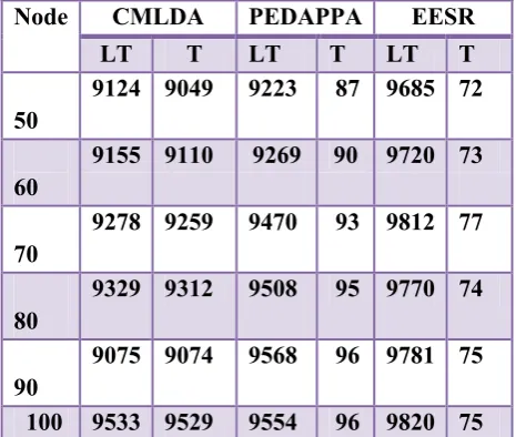
In each experiment, sensors are placed randomly in the field and presented results are averaged of 10 different experiments with same network parameters. We compare the network lifetime (LT) and number of distinct routing trees (T), generated by EESR,CMLDA and PEDAPPA protocols. Table 1 and 2 shows EESR performance for 50×50m2 network field when base station is within and outside of the network respectively.

For all network sizes, our EESR protocol outperforms CMLDA and PEDAPPA in terms of network lifetime. Moreover, EESR also minimizes number of routing CMLDA varies with cluster size. Too small cluster size of CMLDA turns to MLDA which results better lifetime with the cost of high time complexity. On the other hand, large cluster size in CMLDA behaves as traditional spanning tree and looses performance. For all experiments, we set the cluster size of 8 and 10 nodes and average results are taken. As the base station moves away from the network, EESR achieves better lifetime with slight increase in number of distinct trees then PEDAPPA.[7]

Table 1:50*50 network, BS at (25,25)

Node CMLDA PEDAPPA EESR

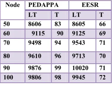
Table 2:50*50 field BS at (150,150)

(7)

PEDAPPPA uses fixed number of rounds for each routing tree. When base station is away from the network, PEDAPPA consumes large amount energy from each tree which results fewer distinct trees with the cost of poor lifetime.[8]

In table 5, we repeat the experiment of table 4 using different initial energy for PEDAPPA and ESSR. In each experiment, 25% of sensors node are randomly selected and equipped with higher initial energy (10J). In all cases, ESSR outperforms PEDAPPA both in lifetime and schedule length.

This experiment gives the indication that ESSR can be used in heterogeneous energy label when few sensors are equipped with higher energy or new sensors are replaced in the network. ESSR adds high power sensors later in the routing tree thus assigning more load to

Table 3:100*100 field BS at (50,50)s

Node CMLDA PEDAPPA EESR

Table 4:100*100 field BS at (200,200)

The strength of EESR can be further observed in dense network. As network gets denser, EESR gives better lifetime using small number of routing trees. As mentioned before, our protocol considers both sending and receiving nodes residual energy in choosing routing path thus works better in dense network. PEDAPPA only considers transmitter residual energy

in edge cost thus ends up assigning higher load to the receiver node and reduces overall performance[5].

Node PEDAPPA EESR

In this paper, we have proposed a spanning tree based multi-hop routing to maximize the lifetime of the network. Where we represented an edge cost function that balance energy among sensors. We also showed that ESSR maximizes network lifetime using limited number of routing trees. We presented our simulation results which shows significant improvement over existing protocols. We showed that our algorithm works better in dense network where receiving energy consumption plays a significant impact to maximize network lifetime. While our approach mainly concerns to extend network lifetime it also tries to generate small schedule size. As a continuation of this work, we are exploring a situation when nodes are not in same transmission range. In future, we will also investigate to maximize network lifetime for heterogeneous network where sensed data are not correlated and aggregation is not possible.

V. REFERENCES

[1]. Mani B. Srivastava Curt Schurgers. Energy

efficient routing in wireless sensor networks. MILCOM’01, pages 357–361, October 28-31 2001.

[2]. I. Matta V. Erramilli and A. Bestavros. On the interaction between data aggregation and topology control in wireless sensor networks. In Proc. of SECON,, pages 557–565,, Oct 2004. [3]. S. Bandyopadhyay and E. J. Coyle. An energy

(8)

wireless sensor networks. In Proceedings of the IEEE Conference on Computer Communications (INFOCOM), 2003.

[4]. S. Ghiasi, A. Srivastava, X. Yang, and M. Sarrafzadeh. Optimal energy aware clustering in sensor networks. Sensors, 2:258–259, 2002.

[5]. Anathan P. Chandraskan Wendi B. Heinzelman

and Hari Blakrisshnan. An application-specific protocol architecture for wireless microsensor

networks. IEEE Trans. on Wireless

Communications, 1(4):660–670, OCT 2002.

[6]. Konstantinos Kalpakis Koustuv Dasgupta and

Parag Namjoshi. An efficient clustering-based heuristic for data gathering and aggregation in

sensor networks. In IEEE Wireless

Communications and Networking Conference, 2003.

[7]. Koustuv Dasgupta Konstantinos Kalpakis and

Parag Namjoshi. Maximum lifetime data gathering and aggregation in wireless sensor networks. In IEEE International Conference on Networking, pages 685–696, August 2002.

[8]. Daniel Kofman Ravi Mazumdar Ness Shroff

Vivek P. Mhatre, Catherine Rosenberg.

[9]. Nandini.M.D.S, Kiruthika.M “Life Time

Balanced Routing Algorithm for Wireless Sensor Networks”, IJARCSMS published 2014.