A
s
tudy on the evaluation of the geoid-qua
s
igeoid
s
eparation term over
Paki
s
tan with a
s
olution of fir
s
t and
s
econd order height term
s
Muhammad Sadiq, Zulfiqar Ahmad, and Gulraiz Akhter
Department of Earth Sciences, Quaid-i-Azam University, Islamabad Post Code 45320, Pakistan
(Received December 27, 2007; Revised November 11, 2008; Accepted January 6, 2009; Online published August 31, 2009)
An attempt has beenmade to evaluate the geoid-quasigeoid separation termover Pakistan by using solutions of terms involving first and second order terrain heights. The first term, involving the Bouguer anomaly, has a significant value and requires being incorporated in any case for determination of the geoid fromthe quasigoidal solution. The results of the study show that the second termof separation, which involves the vertical gravity anomaly gradient, is significant only in areas with very high terrain elevations and reaches amaximumvalue of 2–3 cm. The integration radius of 18 kmfor the evaluation of the vertical gravity anomaly gradient was found to be adequate for the near zone contribution in the case of the vertical gravity anomaly gradient. The Earth Gravity Model EGM96 height anomaly gradient terms were evaluated to assess themagnitude of themodel dependent part of the separation term. The density of the topographic masses was estimated with the linear operator of vertical gravity anomaly gradient using the complete Bouguer anomaly data with an initial arbitrary density of 2.67 g/cm3 to study the effect of variable Bouguer density on the geoid-quasigeoid separation. The density
estimates seemto be reasonable except in the area of very high relief in the northern parts. The effect of variable density is significant in the value of the Bouguer anomaly-dependent geoid-quasigeoid separation and needs to be incorporated for its true applicability in the geoid-quasigeoid separation determination. The geoid height (N) was estimated fromthe geoid-quasigeoid separation termplus global part of height anomaly and terrain-dependant correction terms. The results were compared with the separation termcomputed fromEGM96-derived gravity anomalies and terrain heights to estimate itsmagnitude and the possible amount of commission and omission effects.
Key words: Geoid, quasigeoid, C1 &C2 correction terms, gravity anomaly, height anomaly, vertical gravity
anomaly gradient.
1.
Introduction
Most of the modern geodetic boundary value problems provide quasigeoid as its solution. The geoid-quasigeoid separation term is then required for the determination of geoid in areas where height datumis based on the
ortho-metric height system. It is well known that rigorous
deter-mination of the geoid requires knowledge of themass dis-tribution of topography above the geoid. To avoid this prob-lem, Molodenskyet al.(1962) discarded the geoid and in-troduced a new surface, the quasigeoid, in which the geoidal undulation is replaced by height anomaly. The determ ina-tion of height anomaly involves no assumption of its density in the computation, unlike the geoidal undulation (N). The geoid-quasigeoid separation termcan then be used for the computation of the geoid fromthe quasigeoid.
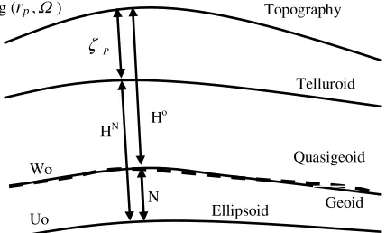
The separation between the quasigeoid height (ζp) and
the geoid height (N) is derived in two different ways. Firstly, the difference between the orthometric height and the normal height yields the separation term. Secondly, the difference of the results of two Stokes formulae for the quasigeoid and the geoid can be used to achieve the purpose
Copyright cThe Society of Geomagnetismand Earth, Planetary and Space Sci-ences (SGEPSS); The Seismological Society of Japan; The Volcanological Society of Japan; The Geodetic Society of Japan; The Japanese Society for Planetary Sci-ences; TERRAPUB.
(Heiskanen and Moritz, 1967; Sj¨oberg, 1995). The geoid is an equipotential surface of the Earth that corresponds to
mean sea level, whereas the quasigeoid is a geometrical sur-face referred to as a normal height system. The geoid un-dulation N is the separation between the ellipsoid and the geoid measured along the ellipsoidal normal. The height anomaly (ζp) is the separation between the reference
ellip-soid and quasigeoid along the ellipellip-soidal normal. There is a similar concept of orthometric heights (Ho)measured along
the plumb line, whereas normal heights (HN) aremeasured
along the ellipsoidal normal. These reference surfaces are shown in Fig. 1.
The geoidal heights can also be computed fromglobal gravity field models, as studied by Rapp (1971, 1994a, b, 1997), who examined different procedures for geoidal height computations using spherical harmonic coefficients of the global Earth gravitymodels. The difference in height anomaly ζp and geoidal-height N and a height anomaly
gradient correction termcan be used to achieve this pur-pose. Sj¨oberg (1995) has proposed this as an ‘indirect’
method; which was further investigated by Nahavandchi (2002) using EGM96 geopotential coefficients (Lemoineet al., 1997). This indirect method for geoid modeling has also been investigated for the entire area of Pakistan using observed gravity data, a global gravitymodel, its
Topography
dependant correction terms, and digital elevation models in addition to quantification of the difference between the geoid and height anomaly. It is a known fact that the global vertical datum, i.e. globalmean sea level or geoid and local
mean sea leveling data, has as an offset/bias (Lisitzin, 1974; Torge, 2001). This bias comes fromthe external harmonic series when applied to the geoid within the topographic
masses as well as fromthe errors in the GPS and leveling data. Additionally, it has its source frompermanent ocean dynamic topography (PODT) andmean sea level changes (Torge, 2001). Sj¨oberg (1977, 1994) pointed out this bias and Sj¨oberg (1994, 1995), Vaniceket al.(1995), and Naha-vandchi and Sj¨oberg (1998) derived different terms to han-dle this bias, which is called the topographic correction for potential coefficients. Here an attempt has beenmade to quantify it through the comparison with local GPS-leveling data as the difference in the standard deviation with respect to global vertical datum.
The observed gravity anomalies, elevation data, and global geopotential model were used in this study. The
model part of the gravity anomaly was computed fromthe EGM96 globalmodel, and the digital elevationmodel data was extracted from GTOPO5 (5-arc min global topogra-phy) and Shuttle Radar Topographic Mission (SRTM30) for the whole area of Pakistan. The terrain correction was applied to the distance of 167 km(∼1.5◦) in the area and added to the Bouguer anomaly to quantify the effect of ter-rain on geoid-quasigeoid separation. The EGM96 global
model is a reasonably good estimate of the global gravity field and height anomalies (Rapp, 1997). Other combined globalmodels, such as the EIGEN-CG01C (Reigberet al., 2004), EIGEN-CG03C and EIGEN-GL04C (F¨osrsteet al., 2005, 2006)models derived fromthe CHAMP and GRACE satellitemissions, are also good enough; however, they have comparable statistics to EGM96 in terms of observed grav-ity and geoid in Pakistan (Sadiq and Ahmad, 2007). The
model part of the geoid-quasigeoid separation termwas de-termined using EGM96 potential coefficients (Lemoineet al., 1997).
The height datumof Pakistan is based on the orthometric height system. Therefore, the final solution should be in the formof the geoid for surveying and other related applica-tions. Pakistan has a variety of terrain distribution due to its vast expanse of land comprising both plain lands tomid
elevation ranges and then to very high Himalayan m oun-tain ranges. The quantification of the maximumpossible value of the geoid to quasigeoid separation is essential due to the fact thatmostmodern geodetic boundary value prob-lems provide the quasigeoid as their final solution, with the exception of the pure Helmert condensation. The basis for this is related to the ways of handling topography in a bet-ter way in thesemethods, e.g., Molodensiki’smethod with RTM and combined RTM/Helmert schemes, among others (Omang and Forsberg, 2000). The focus of this study is
mainly on the estimation of asmaximumas possible com -plete geoid-quasigeoid separation termto be used for the determination of a geoid froma quasigeoidal solution. For this purpose, an initial study was made to investigate the geoid-quasigeoid separation termdependence on elevation by Sadiq and Ahmad (2006) as a part of geoid-quasigeoid separation (Np−ζp)modeling study in Pakistan.
Section 2 provides a brief theoretical background for the evaluation of the geoid-quasigeoid separation term, Sec-tion 3 analyses the test results, and SecSec-tion 4 presents the results with some recommendations.
2.
Brief Theoretical Background
The geoid to quasigeoid separation termis a function of the geoid and quasigeoid in one sense and orthomeric and normal heights in the other sense. This termcan be
deter-mined with adequate accuracy as a difference of the geoid and quasigeoid using terms to the second power of orthom e-tric heights (Sj¨oberg, 1995) by the following relationship.
Np−ζp=
the orthometric height, and γ¯ is the average theoretical gravity along the ellipsoidal normal between the surface of the geocentric reference ellipsoid and the telluroid.
Rapp (1997) pointed out thatζpis dependent on the
gra-dients of radius vectorrp and height as a function of the
first order height term. The valueζ0 at the ellipsoidal
sur-face needs to be corrected to obtainζ values at P.
ζp=ζ0(ϕ, λ,rE)+∂ζ
whereh is the ellipsoidal height of point P andrE is the
ellipsoidal radius. We can write the final formfor geoid-quasigeoid separation as (Rapp, 1997; Nahavandchi, 2002)
N(ϕ, λ)=ζ0(ϕ, λ,rE)+C1(ϕ, λ)+C2(ϕ, λ) (3)
whereζ0 is the height anomaly at the ellipsoidal surface,
andϕandλare the geodetic latitude and longitude, respec-tively
Here, orthometric height can be used instead of ellipsoidal height without any loss of accuracy (Rapp, 1997)
The following conventionmay be adopted for naming the terms of Eqs. (4) and (5),
C1(ϕ, λ)=C11(ϕ, λ)+C12(ϕ, λ) (6)
and
C2(ϕ, λ)=C21(ϕ, λ)+C22(ϕ, λ). (7)
The solution of Eq. (4) can be determined using the rela-tionship for the height anomaly (Rapp, 1997) with spherical harmonic expansion to degree and order 360 as below
ζ0(ϕ, λ,rE)=
whereγ is the normal gravity at the ellipsoid anda is its semi-major axis,C¯nmS¯nmare fully normalized potential co-efficients of degreenand orderm, andP¯nmis fully norm al-ized Legendre function. The first and second termof Eq. (4) can be determined using Eq. (8) as follows.
∂ζ
determined by Eqs. (9) and (10) using height data and gravity-mass constant G M with the definition of Wo
(Bursa, 1995) in a non-tidal system. Here, we have used 3.986004418E+1014m3s−2forG Min order tomake
con-sistent calculations with respect to the tidal systemused. The first termof Eq. (5) is simple to compute. The sec-ond term, the height gradient of free air anomaly, requires special solution techniques and is given by Heiskanen and Moritz (1967) as
wherelo is the spatial distance between the computation
point P and the running point,Ris the average earth radius, andσ is the unit sphere. The planar solution of Eq. (2), as given by Heiskanen and Moritz (1967), can be written as
∂gF
wheres0 is the constant linear distance (here it is the grid
interval of the gridded data), andgx xandgyyare the second order horizontal derivatives of the free air gravity anomaly.
The horizontal second order derivatives were calculated fromthe gridded free air anomaly data at 5arcminute grid intervals.
The approximation of the vertical gravity anomaly gra-dient with Eq. (12) is not very accurate, but it can be im -proved with numerical integration for greater integration radii. For this purpose, the solution of Eq. (11) was de-termined numerically using Newton-Cotes formulae after solving the singular integral in the planar approximation. The planar/flat Earth approximation of the vertical gravity anomaly gradient is expressed as (Heiskanen and Moritz, 1967; Bian and Dong, 1991; Bian, 1997).
∂g
planar coordinates of themoving point. The solution for the innermost area,−2a <x <2a,−2a <y <2a, was im -plemented on the gridded data with a planar approximation with a grid interval ‘a’. The final solution for the vertical gravity anomaly gradient comes out to be
∂g
The average integration radius corresponding to the Newton-Cotes formula for n = 4 with a grid interval of 5 arc min was used in this study. Additionally, the even orders of the Newton-Cotes integration yield exact results. This is due to the reason that the fourth order was found to be enough for estimating of the vertical gravity anomaly gradient through Eq. (14) in the innermost zone formedium
elevation ranges (Sadiqet al., 2008). In addition to this, it is also known that the vertical gravity anomaly dependent
C22, i.e., second termof Eq. (1) is ofmuch lessmagnitude
Table 1. Statistics of the input parameters for the computation of the geoid-quasigeoid separation term.
Parameter Min Max Mean Std. dev.
Altitude (m) −3836.2 6143.8 374.45 1767.74 Bouguer Anomaly (mgal) −559.85 132.2 −91.69 114.03 Free air Anomaly (mgal) −290.97 256.25 −39.09 76.512 Terrain correction (mgal) −64.264 229.13 16.92 27.04
3.
Data Processing Strategy and Analysis
of
Re-sults
The gravity data for the numerical investigation was taken from the GETECH database (GETECH, 1995) for Bouguer gravity anomalies over Pakistan with a 5 grid interval. The digital elevation model of GTOPO5 and SRTM30 were also available for the computation terrain-related gravity field parameters. The topographic heights vary from3836.2 to 6143.8mwithin the study area. Since GTOPO5 elevation data were used for the evaluation of Bouguer anomaly, the free air anomaly was computed by the back transformation of the procedure implemented for the determination of the Bouguer anomaly. The Bouguer gravity anomaly varies from−559.85mgal to 132.2mgal with a constant topographic density of 2.67 g/cm3. The free air anomaly ranges from−290.97 to 256.25mgal. The terrain-corrected Bouguer anomaly is preferred for the es-timation of the C21 correction term. To this end, the
ter-rain correction was estimated via prismintegration using the GRAVSOFT (2005) programand was computed by us-ing a 30-arc second resolution SRTM30 grid along with in-termediate (5-arcmin grid) and reference grid (30-arcmin grid). It varies from−64.264 to 229.133mgal in the study area. The theoretical normal gravity (i.e., γ) at the ellip-soidal surface was computed using Somigliana’s formula. The statistics of input gravity field parameters is shown in Table 1.
For better management and data manipulation
require-ments, the whole area of Pakistan was divided into two parts, namely PKGRD1 and PKGRD2, for the estimation of the C22 term using free air gravity anomalies. The
data around the Pakistan were filled with EGM96 free air anomaly data to make the above two grids as regular and rectangular as possible and therefore useful for computating first and second order horizontal derivatives. These deriva-tives were used in Eq. (14) to compute the vertical grav-ity anomaly gradient, which was further used in Eq. (5) to compute theC22part of the geoid-quasigeoid separationC2
term.
The global geopotential model-dependent C1 term
(Eqs. (9) and (10)) was computed by employing the global gravity model and digital elevation data (GTOPO5 and SRTM30). To this end, the EGM96model with its geopo-tential coefficients was used for themaximumdegree of ex-pansion, i.e., degree and order of 360. The ground gravity data-dependentC2termwas computed while using the
digi-tal elevationmodel and ground gravity free air and Bouguer gravity anomalies. The computation ofC21 and C22 was
performed using actual data of the GETECH grid avail-able within the GETECH database along with terrain
cor-rections.
3.1 Development of topographic density model
TheC21part of the separation term, which is dependent
on the Bouguer anomaly, has a built-in supposition of con-stant density of 2.67 g/cm3. The use of constant density
introduces errors into the reduced gravity anomalies (e.g., simple Bouguer anomaly and its terrain-corrected version) and, consequently, in the geoid-quasigeoid separation and geoid itself.
Several studies have been conducted using laterally vary-ing topographic densitymodels in gravimetric geoid com -putations (e.g., Martinecet al., 1995; Kuhtreiber, 1998; Pa-giatakis and Armenakis, 1999; Tziavos and Featherstone, 2000; Huang et al., 2001; Hunegnaw, 2001). Different approaches can be used for the development of a density
model in a particular area. The first, but rather difficult, ap-proach is the directmeasurement and collection of samples. Thismethod has limitations due to inaccessibility andmay not be representative. The other well-known geophysical
method is the use of the density profile approach (Nettleton, 1971). An extension of thismethod is density estimation using a linear least squares regression for the distributed over an area (Helmut, 1965). One important geophysical technique is the well-logs investigationmethod. From a practical point of view, it is very expensive and is usually used only for special exploration projects (e.g., oil explo-ration, etc.). The information derived fromgeologicalmaps can be utilized for establishing topographic densitymodels. Various researchers around the world (see Martinec, 1993; Pagiatakis and Armenakis, 1999; Kuhn, 2000a, b; Tziavos and Featherstone, 2000; Huanget al., 2001; Kiamehr, 2006) have successfully used geologicalmaps to generate density
models. A 3-D digital density model is usually needed to give a better description of the topographicmasses, but the development of such amodel can be very difficult or almost impossible. Nevertheless, an approximate densitymodel would improve the gravity reduction in a precise geoid de-termination rather than assuming an unrealistic constant density model (Kiamehr, 2006). In addition to this, true seismic velocities of the crustal layer can be very well em -ployed for estimating crustal rock density (Nafe and Drake, 1963). Another workable approachmay be Fractal dim en-sion estimation fromBouguer anomaly data for density de-termination (Thorarinsson and Magnusson, 1990).
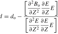
In the present study, an attempt was alsomade to evalu-ate and estimate the effect of the true average density on geoid-quasigeoid separation in the maximum part of the study area. To this end, the generalized procedure of linear regression (Helmut, 1965) was implemented for the evalu-ation of Bouguer density using the Bouguer anomaly and terrain correction-dependant term(Eq. (16)) in the follow-ing form.
where Bo is the arbitrary Bouguer anomaly using density
Table 2. The topographic densities determined using the generalized Nettleton Procedure.
Grid description Density (g/cm3) Grid-1 22.0◦–25.7◦N 60.0◦–64.0◦E 2.643 Grid-2 22.0◦–25.7◦N 64.0833◦–69◦E 2.728 Grid-3 24.0◦–27.667◦N 69.0833◦–71.2◦E 2.632 Grid-4 25.8◦–30.25◦N 61.0◦–65.667◦E 2.661 Grid-5 27.75◦–30.25◦N 65.75◦–71.25◦E 2.634 Grid-6 30.0◦–32.0◦N 66.0◦–69.0◦E 2.654 Grid-7 30.333◦–32.25◦N 69.0◦–71.0◦E 2.807 Grid-8 27.833◦–34.2◦N 71.33◦–75.5◦E 2.625 Grid-9 32.333◦–34.5◦N 69.0◦–75.5◦E 2.848 Grid-10 34.3◦–37.0◦N 70.5◦–77.0◦E 2.929
computation of the vertical gradient of the different terms
mentioned in Eq. (15). The term‘E’ is defined by
E =T −0.04193∗Ho (16)
where ‘T’ is terrain correction and ‘Ho’ is orthometric
height. For estimation of the true average density ‘d’, linear operators of first and second vertical derivative of the grav-ity anomaly were applied on the gridded data. The second termof Eq. (15) was determined for true average density ‘d’ for each grid, asmentioned in Table 2.
The study area was therefore divided into different grids with suitable dimensions (total of ten sub-grids for the Pak-istan area) for data handling in the planar approximation and more representative density calculations. The com -puted average density appears to fall towards the higher side for grids 7, 9, and 10, which occurs due to the high relief and steep slopes in the northern parts. This originates from
the inherent characteristics of themethod resulting fromthe distribution of terrain and gradient of gravity anomalies.
3.2 Analysisof results
The procedure of computation of geoid to quasigeoid separation term has been implemented and quantified for themaximumpossible area of Pakistan based on observed gravity andmodel datasets. The work done by Rapp (1997) and Nahavandchi (2002), with minor modifications, has been adopted in a study area which has a very high and rugged terrain. In addition to this, estimation of Bouguer density wasmade within Pakistan to better evaluate its ef-fect on density-dependant geoid-quasigeoid separation, i.e.,
C21.
3.2.1 The estimation of the C2 term (C21 plusC22)
The planar approximation was applied for the solution of the singular integral of the vertical gravity anomaly gradi-ent for the estimation of theC22 term. The complete geoid
to quasigeoid separation termas the sumofC1 andC2 in
Eq. (3) was computed fromEqs. (4) and (5) after the indi-vidual terms had been determined using Eqs. (8), (9), (10), and (14). The global part of correctionC1 was computed
fromthe EGM96 global gravitymodel.
The terrain-corrected Bouguer anomaly and topographic height were used for the calculation of theC21 term. The
variation of this termis−3.2637 to 0.0096mwith a stan-dard deviation of 0.4929mwhile using a constant density of 2.67 g/cm3. ThisC
21termis found to bemaximum
con-tributor towards the total effect of the geoid-quasigeoid
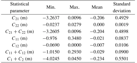
sep-Table 3. The statistics of different parts of the complete geoid-quasigeoid separation term(C21with constant density of 2.67 g/cm3).
Statistical
Min. Max. Mean Standard
parameter deviation
C21(m) −3.2637 0.0096 −0.206 0.4929 C22(m) −0.0237 0.0279 0.000 0.0019 C21+C22(m) −3.2605 0.0096 −0.204 0.4898 C11(m) −0.976 0.3480 −0.021 0.0837 C12(m) −0.0690 0.0000 −0.007 0.0106 C11+C12(m) −1.0150 0.2930 −0.029 0.0900 C1+C2(m) −4.0245 0.0450 −0.234 0.5501
Table 4. The statistics of different parts of the complete geoid to quasi-geoid separation term(C21computed with variable density from Ta-ble 2).
Statistical
Min. Max. Mean Standard
parameter deviation
C21(m) −3.580 0.0096 −0.220 0.5375 C22(m) −0.0237 0.0279 0.000 0.0019 C21+C22(m) −3.577 0.0096 −0.220 0.5374 C11(m) −0.976 0.3480 −0.021 0.0837 C12(m) −0.0690 0.0000 −0.0076 0.0106 C11+C12(m) −1.0150 0.2930 −0.0291 0.0900 C1+C2(m) −4.329 0.0391 −0.2495 0.597
aration termdue to the Bouguer plate effect, as shown in Fig. 2.
The variable density for different grids suitably selected was also used for grids 1–10 (Table 2). The estimates of densities for grids 7, 9, and 10 seemto be relatively higher. The density values for the remaining seven grids are as ex-pected and seemto be realistic estimates. The estimation of theC21termfromthe Bouguer anomaly wasmade with
constant as well as variable density data. The effect of vari-able densities appears to be considervari-able (Tvari-ables 3 and 4) and needs to be incorporated for better modeling of this term. Themean and standard deviation differences of the
C21termfor the two cases are 13.9 and 44.6mm. This,
how-ever, requires that the densitymodeling be verified by some other independentmethod, such as computed fromFractal dimension estimation of Bouguer densities (Thorarinsson and Magnusson, 1990) and/or seismic velocities of topo-graphicmasses (Nafe and Drake, 1963), among others. The results of variable and constant density are shown in Ta-bles 3 and 4. The second part of theC2term, i.e.,C22, was
computed using free air gravity anomaly data on the grid of 5×5. The whole study area was divided into two parts, keeping inmind the distribution of data and extensions. The computed first and second horizontal derivatives were used in Eq. (14) to compute the vertical gravity anomaly gradi-ent, which was then used in Eq. (5) to compute this second part ofC2term.
During the computation of the vertical gravity anomaly gradient, it was observed that Newton-Cotes formula for
n = 4 seems to be adequate for practical purposes for the evaluation of theC22 term. The variation in theC22 term
over the whole study area ranges from−23.7 to 27.9mm
aly-Table 5. The statistics of different parts of complete geoid to quasigeoid separation termand EGM96 height anomaly (C21determined using the EGM96 correction coefficients set).
Statistical parameter Min. Max. Mean Std. dev.
EGM96 height anomaly (m) −54.08 −17.19 −39.263 7.92
C21(EGM96 Corr. Coeff.) (m) −3.42 0.05 −0.220 0.557
C22(m) −0.024 0.0279 0.0000 0.0019
C21+C22(m) −3.419 0.0499 −0.220 0.5568
C11(m) −0.976 0.3480 −0.021 0.0837
C12(m) −0.069 0.0000 −0.0076 0.0106
C11+C12(m) −1.0150 0.2930 −0.0291 0.0900
C1+C2(m) −4.0647 0.167 −0.249 0.6189
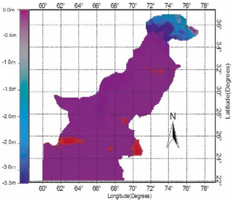
Fig. 2. The image plot of theC21part of the geoid-quasigeoid separation.
Fig. 3. The image plot of theC22part of geoid-quasigeoid separation.
dependant termC21. This shows that theC22part is
insignif-icant in the completeC2termand that the overall statistics
of theC2 termdoes not change verymuch because it has
been statistically hidden by the major part of C21, as has
been shown in Fig. 3.
3.2.2 Estimation of theC1term (C11plusC12) The C1termwas computed fromthe global geopotential
coeffi-cients of EGM96 fromthe expansion up to order and 360◦ with height anomaly gradient terms using Eqs. (9) and (10) and implemented with somemodifications in the software F477S.FOR (Rapp, 1982). After this implementation, the programcalculates theseC11 andC12 terms at the surface
of earth. The gradient term C1 for the geoid-quasigeoid
separation requires the data of topographic height and the potential coefficient of the recent earth gravitymodel.
The total C1 term (sum of C11 and C12) varies from −1.032 to 0.293 min the whole study area. The overall effect on the total geoid-quasigeoid separation termis found to be additive in general, as it is evident fromthe statistics given in Tables 4 and 5 andmaps shown in Figs. 4, 5, and 6. The contour pattern of theC1termshows a similar trend of
increase inmagnitude fromlow land areas towards the high
mountains, as it is observable in theC21andC22terms.
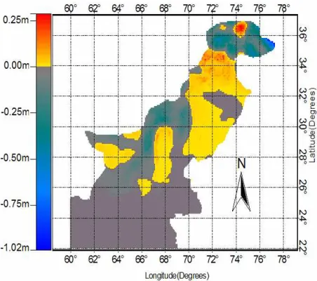
Themodel part of the geoid-quasigeoid separation term
(Fig. 7) was computed to assess itsmagnitude in com par-ison with one computed in the scheme above. This sepa-ration termwas computed using EGM96 model (Lemoine
et al., 1997) with the geopotential coefficients and geoid-quasigeoid correction coefficients determined by Rapp (1997) fromthe values of theC1andC2terms using global
30×30 gravity anomaly data; for details, see the paper fromRapp (1997). The harmonic expansion for the correc-tion termwasmade to 360◦ so that the corresponding cell size is 30×30tomatch the resolution with EGM96. With this information now available, theC1 and C2 terms can
be evaluated on a global grid. This correction termrefers to the WGS84 ellipsoid. The computation of C1 andC2
wasmade using programF477.FOR (Rapp, 1982). These data however, aremissing theC12 andC22 terms. It is
ob-servable fromour results that it does not differmuch from
the totalC2 termobtained fromobserved gravity data
ex-cept the height anomaly gradient termC12andC22obtained
fromthe free air vertical gravity anomaly gradient. This re-sult shows that the EGM96 earth gravitymodel-basedC21
termcorresponds nearly to GTECH data in Pakistan area computed with variable densities. The comparison of Ta-bles 3 and 5 clearly shows that EGM96-dependant geoid-quasigeoid separation is closer to variable density based re-sults from observed data rather than for constant density. Statistics for the geoid to quasigeoid separation termand
deter-Fig. 4. The image plot of theC2part of the geoid-quasigeoid separation.
Fig. 5. The image plot of theC1part of the geoid-quasigeoid separation.
mination of geodal height (N) fromthe height anomalyζp
and additionalC1 andC2 terms dependent on H and H2
as mentioned in Eqs. (1), (2), and (3) in Section 2. This scheme has been proposed to be indirect geoid determ ina-tionmethod based on gravimetric data (Sj¨oberg, 1995; Na-havandchi, 2002; section 3). For comparison purposes, we computed the geoid using thismethod and compared it with GPS-leveling geoid data at 35 selected points. The height anomaly was computed using Eq. (8) at the ellipsoidal sur-face by employing the EGM96 potential coefficients up to order and degree 360 at the locations of the GPS-leveling data points. The C1 andC2 terms were computed at the
same locations using the results of Eqs. (4) and (5), respec-tively.
The GPS-leveling geoidal heights (N) were computed using the difference between ellipsoidal heights (h),m ea-sured with the differential global positioning system
(DGPS), and orthometric heights (H), obtained from
pre-Fig. 6. The image plot of the sumofC1 andC2 of geoid-quasigeoid separation.
Fig. 7. The image plot of geoid-quasigeoidC term separation using EGM96 data.
cise leveling data with simple relation
N =h−H. (17)
The GPS ellipsoidal height data were collected and pro-cessed by the Survey of Pakistan and was connected to the high precision first order leveling network already estab-lished (Noor et al., 1997). The GPS bench marks were comprised ten GPS control points, and the other 25 points belonged to the Pakistani first order geodetic network. The processed DGPS 3-D coordinate data have amaximum er-ror of 10 cmin the ITRF94 reference frame (Nooret al., 1997). The high precision leveling data has amaximum
error of 2 cmas absolute. The statistics of differences be-tween the computed gravimetric and GPS-Leveling geoidal heights at 35 stations are shown in Table 6.
An-Table 6. Statistics of differences between gravimetric and GPS-leveling derived geoid heights for 35 GPS-leveling stations.
Model type Min. Max. Mean Std. dev.
Difference b/w GPS Leveling & gravimetric geoids (m) −1.741 1.477 −0.318 0.773 Difference b/w GPS Leveling & EGM96 geoids with EGM96 correction termadded (m) −1.235 2.002 0.206 0.775
derson, Neil’s Bohr Institute). However, this height bias value can not be representative of the total datum height offset due to insufficient GPS-leveling data (only 35 num -bers) and not well-distributed data in the Pakistan area in addition to the other inherent errors of geodeticm
easure-ments. Since both gravimetric as well as EGM96-derived results are representative of the global datum, the difference is almost the same in terms of local GPS-leveling data. A
maximumdifference of−1.741mhas been computed with respect to the gravimetric and GPS-leveling geoid. The rea-son behind this differencemight be associated with errors in the GPS-leveling data, heights derived fromGTOPO5, observed gravity data, and errors in themodeling of den-sity in the determination of the geoid-quasigeoid separation term, in addition to the constant height offset between local and global vertical datums in the Pakistan area. In addition to this, the geoidal height determined through the height anomaly has shown good agreement with the GPS-leveling data, though some high-frequency information, i.e., terrain effects etc, is not present in this approach (Nahavandchi, 2002). This method can give better results by increasing the accuracy of potential coefficientmodels through the ad-dition of high-frequency information fromland gravity and terrain data and increasing themaximumdegree of expan-sion in future global geopotentialmodels.
4.
Conclusion and Recommendations
This study focuses on the computation and assessment of the complete geoid to quasigeoid separation termfor the selection of the onward geoid determinationmethod. Pak-istan has an orthometric height system, therefore this cor-rection termwill facilitate the determination of the geoid in Pakistan more precisely, if the height anomaly is cal-culated from observed gravity data using the solution of the geodetic boundary value problembased on Moloden-siky’s approach. The geoidal heights determined through height anomaly and terrain-dependant correction terms has demonstrated relatively good agreement to GPS-leveling data in comparison to those computed from the EGM96
model and its geoid-quasigeoid correction coefficients set. The results of our comparison confirm the difference of global vertical datumand local GPS-leveling datumto be of the order of 0.7 m in the sense of height bias; how-ever, this comparison is not complete in the sense that GPS-leveling data were not sufficient and well distributed. This comparison requiresmore GPS-leveling data in the whole area of Pakistan for better confidence on the derived re-sults. The results might also be improved by calculating the height anomaly component fromobserved gravity data. Additional benchmark data are required to obtain the bet-ter comparison results. Some additional work is required for the calculation of this separation termusing more re-dundant and reliable density estimates by some other
work-able independentmethod, such as the Fractal dimension of the Bouguer anomaly or fromseismic velocities data to es-timate the Bouguer density evaluation.
Acknowledgments. Higher Education Commission of Pakistan is highly acknowledged for sponsoring this study under the in-digenous Ph.D. program at the Department of Earth Sciences Quaid-i-Azam University (QAU) Islamabad, Pakistan. The Di-rectorate General of PetroleumConcessions (DGPC), Ministry of Petroleum and Natural Resources Islamabad, GTECH, Univer-sity of Leeds, UK and Survey of Pakistan are also acknowledged for providing the gravity, elevation, and GPS-leveling data of the study area to the Department of Earth Sciences, QAU, Islamabad for this research. The authors also appreciate the valuable sugges-tions and comments fromthe associate editor and two anonymous reviewers.
References
Andersen, O. B., L. Anne, Vest, and P. Knudsen, The KMS04 Multi-Missionmean Sea Surface,Proceedings of the Workshop GOCINA: Im-proving modeling of ocean transport and climate prediction in the North Atlantic region using GOCE gravimetry, April 13–15, 2005, Novotel, Luxembourg, 2005.
Bian, S., Some cubature formulas for singular integrals in geodesy,J. Geod.,71, 443–453, 1997.
Bian, S. and X. Dong, On the singular integration in physical geodesy,
Manuscr. Geod.,16, 283–287, 1991.
Bursa, M.,Report of Special Commission SC3, Fundamental constants, International Association of Geodesy, Paris, 1995.
F¨osrste, C., F. Flechtner, R. Schmidt, U. Meyer, R. Stubenvoll, F. Barthelmes, R. K¨onig, K. H. Neumayer, M. Rothacher, Ch. Reigber, R. Biancale, S. Bruinsma, J.-M. Lemoine, and J. C. Raimondo, A new high resolution global gravity fieldmodel derived fromcombination of GRACE and CHAMPmission and altimetry/gravimetry surface gravity data, Poster presented atEGU General Assem. 2005, Vienna, Austria, 24–29, April, 2005, 2005.
F¨osrste, C., F. Flechtner, R. Schmidt, R. K¨onig, U. Meyer, R. Stubenvoll, M. Rothacher, F. Barthelmes, H. Neumayer, R. Biancale, S. Bruinsma, J.-M. Lemoine, and S. Loyer, Amean global gravity fieldmodel from
the combination of satellitemission and altimetry/gravimetry surface data—EIGEN-Gl04C,Geophys. Res. Abst.,8, 03462, 2006.
GETECH,GETECH report on South East Asia Gravity project (SEAGP), GETECH Group plc., Kitson House, Elmete Hall Elmete Lane, Round-hay University of Leeds, LS8 2LJ, U.K., 1995.
GRAVSOFT, A systemfor geodetic gravity fieldmodelling, C. C. Tsch-erning, Department of Geophysics, Juliane Maries Vej 30, DK-2100 Copenhagen N. R. Forsberg and P. Knudsen, Kort og Matrikelstyrelsen, Rentemestervej-8, DK-2400 Copenhagen NV, 2005.
Heiskanen, W. A. and H. Moritz,Physical Geodesy, Freeman, San Fran-cisco, 1967.
Helmut, L., A generalized formof Nettletons’s density determination,
Geophys. Prospect.,15, 247–258, 1965.
Huang, J., P. Vanicek, S. Pagiatakis, and W. Brink, Effect of topographical
mass density variation on gravity and geoid in the Canadian Rocky Mountains,J. Geodyn.,74, 805–815, 2001.
Hunegnaw, A., The effect of lateral density variation on local geoid
deter-mination,Proc. IAG 2001 Sci. Assem., Budapest, Hungary, 2001. Kiamehr, R., The impact of lateral density variationmodel in the determ
i-nation of precise gravimetric geoid inmountainous areas: a case study of Iran,Geophys. J. Int.,167, 521–527, 2006.
Kuhn, M., GeoidBestimmung unter verwendung verschiedener dichtehy-pothesen. Deutsche Geodatische Kommission, inDissertationen, Heft Nr. 520, edited by C. Reihe, Munchen, Gaermany, 2000a.
Kuhtreiber, N., Precise geoid determination using a density variation
model,Phys. Chem. Earth,23(1), 59–63, 1998.
Lemoine, F. G., D. E. Smith, R. Smith, L. Kunz, N. K. Pavlis, S. M. Klosko, D. S. Chinn, M. H. Torrence, R. G. Williamson, C. M. Cox, K. E. Rachlin, Y. M. Wang, E. C. Pavlis, S. C. Kenyon, R. Salman, R. Trimmer, R. H. Rapp, and R. S. Nerem, The development of thr NASA, GSFC and NIMA joint geopotentialmodel, inGravzly, Geozd, and Marzne Geod., edited by Segawa, Fugimoto and Okubo, IAG Synzposza 117, Springer-Verlag, Berlin, 461–470, 1997.
Lisitzin, E.,Sea level changes, Elsevier, Amsterdam, 1974.
Martinec, Z., Effect of lateral density variations of topographicalmasses in view of improving geoidmodel accuracy over Canada,Contract report for Geodetic Survey of Canada, Ottawa, Canada, 1993.
Martinec, Z., P. Vanicek, A. Mainville, and M. Veronneau, The effect of lake water on geoidal height,Manuscr. Geod.,20, 193–203, 1995. Molodensky, M. S., V. F. Eremeev, and M. I. Yurkina,Methods for the
study of the external gravitational field and figure of the Earth, Israeli Programfor Scientific Translations, Jerusalem, 1962.
Nahavandchi, H., Two differentmethods of geoidal height determinations using a spherical harmonics representation of the geopotential, topo-graphic corrections and height anomaly-geoidal height difference,J. Geod.,76, 345–352, 2002.
Nahavandchi, H. and L. E. Sj¨oberg, Terrain correction to power H3 in gravimetric geoid determination,J. Geod.,72, 124–135, 1998. Nafe, L. E. and C. L. Drake, Physical properties ofmarine sediments, in
The sea Interscience, edited by Hill, 794–815, 1963.
Nettleton, L. L., Elementary gravity andmagnetic for geologists and
seis-mologists,SEG Monogr. Ser. l,121, 1971.
Noor, E., J. Chen, L. Yulin, and J. Zhang, Report on data process-ing/adjustment regarding “A” & “AB” order GPS networks of Pakistan June 15–24, 1997,Survey of Pakistan Rawalpindi, 1997.
Omang, O. C. D. and R. Forsberg, How to handle topography in practical geoid determination: three examples,J. Geod.,74, 458–466, 2000. Pagiatakis, S. D. and C. Armenakis, Gravimetric geoidmodelling with
GIS,Int. Geoid Serv. Bull.,8, 105–112, 1999.
Rapp, R. H., Methods for the computation of geoid undulations from
potential coe.cients,Bull. Geod.,101, 283–297, 1971.
Rapp, R. H., A FORTRAN Programfor the computation of gravimetric quantities fromhigh degree spherical harmonic expansions,Rep. 334, Dept. of Geodetic Science and Surveying, The Ohio State University, Columbus, Ohio, 1982.
Rapp, R. H., Global geoid determination, inGeoid and Its Geophysical Interpretations, edited by Vanicek and Christou, p. 57–76, CRC Press, Boca Raton. FL, 1994a.
Rapp, R. H., The use of potential coefficientmodels in computing geoid undulations. Intenational School for the determination and use of the geoid,Int. Geoid Serv., DIIAR-Politecnico di Milano, 71–99, 1994b. Rapp, R. H., Use of potential coefficient models for geoid undulation
determinations using a spherical harmonic representation of the height anomaly/geoid undulation difference,J. Geod.,71, 282–289, 1997. Reigber, Ch., P. Schwintzer, R. Stubenvoll, R. Schmidt, F. Flechtner, U.
Meyer, R. K¨onig, H. Neumayer, Ch. F¨orste, F. Barthelmes, S. Y. Zhu, G. Balmino, R. Biancale, J.-M. Lemoine, H. Meixner, and J. C. Raimondo,
A High Resolution Global Gravity Field Model Combining CHAMP and GRACE Satellite Mission and Surface Data: EIGEN-CG01C, 2004. Sadiq, M. and Z. Ahmad, A comparative study of the geoid-quasigeoid
separation termC at two different locations with different topographic distributions,Newton’s Bulletin,3, 1–10, International Geoid Service www.iges.polimi.it, 2006.
Sadiq, M. and Z. Ahmad, On the selection of optimal global geopotential
model for geoidmodeling: a case study in Pakistan,Internal report#11, Dept. of Earth Sciences QAU, Islamabad, 2007.
Sadiq, M., Z. Ahmad, and M. Ayub, Vertical gravity anomaly gradient ef-fect on the geoid-quasigeoid separation and an optimal integration ra-dius in planer approximation,Studia Geophys. Geod., 2008 (submitted). Sj¨oberg, L. E., On the error of spherical harmonic development of gravity at the surface of the Earth,Rep. 257, Department of Geodetic Science, The Ohio State University, Columbus, 1977.
Sj¨oberg, L. E., On the total terrain effects in geoid and quasigeoid determ i-nations using Helmert second condensationmethod,Rep. 36, Division of Geodesy, Royal Institute of Technology, Stockholm, 1994. Sj¨oberg, L. E., On the quasigeoid to geoid separation,Manuscr. Geod.,20,
182–192, 1995.
Thorarinsson, F. and S. G. Magnusson, Bouguer density determination by fractal analysis,Geophys.,55, 932–935, 1990.
Torge, W.,Geodesy, 3rd ed., 2001.
Tziavos, I. N. and W. E. Featherstone, First results of using digital density data in gravimetric geoids computation in Australia, IAG Symposia, GGG2000, Springer Verlag,Berlin Heidelberg,123, 335–340, 2000. USGS,EROS, SRTM30 Digital Elevation Model DATA Center, SIOUX
Fall, SD 57198–0001, http://srtm.usgs.gov/data/obtainingdata.html. Vanicek, P., M. Naja, Z. Martinec, L. Harrie, and L. E. Sj¨oberg, Higher
or-der reference field in the generalized Stokes-Helmert scheme for geoid computation,J. Geod.,70, 176–182, 1995.