R E S E A R C H
Open Access
On the dynamics of new 4D Lorenz-type
chaos systems
Guangyun Zhang
1, Fuchen Zhang
1,2*, Xiaofeng Liao
3, Da Lin
4,5and Ping Zhou
6*Correspondence:
zhangfuchen1983@163.com 1College of Mathematics and
Statistics, Chongqing Technology and Business University, Chongqing, 400067, People’s Republic of China 2College of Mathematics and
Statistics, Southwest University, Chongqing, 400716, People’s Republic of China
Full list of author information is available at the end of the article
Abstract
It is often difficult to obtain the bounds of the hyperchaotic systems due to very complex algebraic structure of the hyperchaotic systems. After an exhaustive research on a new 4D Lorenz-type hyperchaotic system and a coupled dynamo chaotic system, we obtain the bounds of the new 4D Lorenz-type hyperchaotic system and the globally attractive set of the coupled dynamo chaotic system. To validate the ultimate bound estimation, numerical simulations are also investigated. The innovation of this article lies in that the method of constructing Lyapunov-like functions applied to the Lorenz system is not applicable to this 4D Lorenz-type hyperchaotic system; moreover, one Lyapunov-like function cannot estimate the bounds of this 4D Lorenz-type hyperchaos system. To sort this out, we construct three Lyapunov-like functions step by step to estimate the bounds of this new 4D
Lorenz-type hyperchaotic system successfully.
Keywords: hyperchaotic systems; stability; invariant sets; domain of attraction; computer simulation
1 Introduction
In , Lorenzet al. found the famous Lorenz chaotic system, which can be described by the following autonomous differential equations []:
⎧
Since then, chaotic systems have been extensively studied, such as the Rössler system [], Chua’s circuit [], the Chen system [], the Lü system [–], the hyperchaos Lorenz sys-tem [], the Shimizu-Morioka syssys-tem [], the Liu syssys-tem []. Various complex dynamical behaviors of chaotic systems are studied due to its various applications in the field of pop-ulation dynamics, electric circuits, cryptology, fluid dynamics, lasers, engineering, stock exchanges, chemical reactions, etc. [–].
In the recent years, motivated by different applications, much work has been reported in constructing the new chaotic and hyperchaotic models [, , , ]. On the one hand, the hyperchaos theory is still a new field of research. On the other hand, there is no general method to obtain hyperchaotic systems. Compared with chaotic systems, hyperchaotic
systems have at least two positive Lyapunov exponents and, therefore, their lowest di-mension is four. To generate a hyperchaotic system, it is essential to increase the system dimension []. Hyperchaotic systems can be obtained by adding one more state variable to a three-dimensional chaotic system []. In , Liet al. constructed a new chaotic system based on the Lorenz chaotic system []:
⎧
According to the chaotic system (), by introducing a linear feedback controllerwin the first equation, and adding a first-order nonlinear differential state equation with respect tow, one gets a new D Lorenz-type chaotic system as follows:
⎧
The Lyapunov exponents of the dynamical system () are calculated numerically for the parameter valuesa= ,b= ,c= ,d= .,k= .,e= .,h= with the initial state (x,y,z,w) = (., ., ., .). System () has Lyapunov exponents asλLE= ., λLE = .,λLE = ,λLE= –. and the Lyapunov dimension is . for the
parame-ters listed above (see Refs. [] and [] for a detailed discussion of Lyapunov exponents of strange attractors in dynamical systems). This means system () is really a dissipative system, and the Lyapunov dimension of system () is fractional. Thus, system () has two positive Lyapunov exponents and the strange attractor, which means the new system () can exhibit a variety of interesting and complex chaotic behavior. System () has a hyper-chaotic attractor, as shown in Figure and Figure .
In this paper, all the simulations are carried out by using the fourth-order Runge-Kutta method with time-steph= ..
A coupled dynamo system can be described by the following differential equations with appropriate normalization of variables [, ]:
⎧
wherewandwrepresent the angular velocities of the rotors of two dynamos,xandx
represent the currents of two dynamos,qandqare the torques applied to the rotors,u,
u,εandεare positive parameters representing dissipative effects of the disk dynamo
Figure 1 Chaotic attractors of system (2) in 3D spaces witha= 5,b= 20,c= 1,d= 0.1,k= 0.1,e= 20.6,
h= 1 and the initial state (x0,y0,z0,w0) = (3.2, 8.5, 3.5, 2.0).
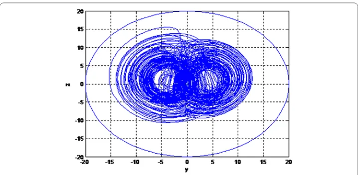
Figure 2 Chaotic attractor of system (2) inyOzplane witha= 5,b= 20,c= 1,d= 0.1,k= 0.1,e= 20.6,
h= 1 and the initial state (x0,y0,z0,w0) = (3.2, 8.5, 3.5, 2.0).
Whenu= .,u= .,q= .,q= .,ε= .,ε= . with the initial
state (x(),x(),w(),w()) = (., ., ., .), system () has a chaotic attractor, as
shown in Figure (also see []).
When u = ., u = .,q = ., q= ., ε = ., ε = . with the initial state
(x(),x(),w(),w()) = (., ., ., ), system () has a chaotic attractor, as shown
in Figure (also see [])
The rest of this paper is organized as follows. The invariant sets of chaotic systems () and () are analyzed in Section . In Section , ultimate bound sets for the chaotic attrac-tors in () and () are studied using Lyapunov stability theory. To validate the ultimate bound estimation, numerical simulations are also provided. Finally, the conclusions are drawn in Section .
2 Invariance analysis for the chaotic attractors in (2) and (3)
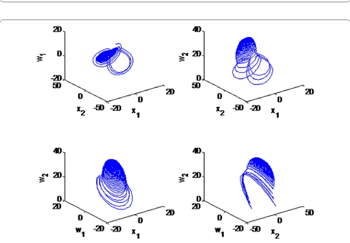
Figure 3 Chaotic attractors of system (3) in 3D spaces withu1= 0.001,u2= 0.0002,q1= 0.19,
q2= 0.21,ε1= 0.15,ε2= 0.15 and the initial state (x1(0),x2(0),w1(0),w2(0)) = (3.2, 8.5, 3.5, 2.0).
Figure 4 Chaotic attractors of system (3) in 3D spaces withu1= 0.2,u2= 0.5,q1= 5.9,q2= 9.15,
ε1= 0.5,ε2= 0.1 and the initial state (x1(0),x2(0),w1(0),w2(0)) = (2.2, 2.0, 10.5, 20).
case on the positivex-axis,y-axis andw-axis for system ().x-axis,x-axis,w-axis and
w-axis are all not positively invariant under the flow generated by system ().
3 Ultimate bound sets for the chaotic attractors in (2) and (3)
Recently, ultimate bound estimation of chaotic systems and hyperchaotic systems has been discussed in many research studies [, , , ]. It is well known that there is a bounded ellipsoid inRfor the Lorenz system which all orbits of the Lorenz system will
for estimation of the fractal dimension of chaotic and hyperchaotic attractors, such as the Hausdorff dimension and the Lyapunov dimension [, ].
Motivated by the above discussion, we will investigate the bounds of the new D Lorenz-type hyperchaotic system () and the disk dynamo system () in this section. The main results are described by Theorem and Theorem .
3.1 Ultimate bound sets for the chaotic attractors in system (2)
Theorem Suppose that∀a> ,h> ,c> ,d> .Let(x(t),y(t),z(t),w(t))be an arbitrary solution of system().Then the set
=
(x,y,z,w)x≤(ad+ke)
R
ad ,y
+z≤R,w≤kR
d
is the ultimate bound set of chaotic system(),where
R=b
θc, θ=min(h,c) > . Proof Define the function
f(z) = –cz+ bz, ∀c> .
Then we can get
max
z∈R f(z) =
b c .
Construct the Lyapunov function
V(X) =V(y,z) =y+z. ()
Computing the derivative ofV(y,z) along the trajectory of system (), we have
dV(y,z)
dt
()
= ydy dt+ z
dz dt
= y(xz–hy) + z(b–xy–cz)
= –hy– cz+ bz
≤–hy–cz–hy–cz+ bz ≤–hy–cz–cz+ bz ≤–θV(y,z) +f(z)
≤–θV(y,z) +b
c
≤–θ V(y,z) –b
θc
Integrating both sides of the above inequality yields
VX(t)≤VX(t)
e–θ(t–t)+
t
t
θRe–θ(t–τ)dτ=VX(t )
e–θ(t–t)+R –e–θ(t–t).
Thus, we can get the following inequality:
VX(t)–R≤V(X) –R
e–θ(t–t).
By the definition, taking the upper limit on both sides of the above inequality ast→+∞ results in
lim
t→+∞V(y,z)≤R
. ()
From inequality (), we can get
|y| ≤R, |z| ≤R. ()
Let us define another function
g(w) = –dw+ kR|w|, ∀d> . Then we can get
max
w∈Rg(w) =
kR
d .
Construct another Lyapunov function
V(w) =w, ()
Computing the derivative of Lyapunov function () along the trajectory of system (), we have
dV(w)
dt
()
= wdw dt
= w(ky–dw)
= –dw+ kyw ≤–dw–dw+ k|y||w| ≤–dw–dw+ kR|w| ≤–dw+g(w)
≤–dw+k
R
d
≤–d V(w) –
kR
d
Similarly, taking the upper limit on both sides of the above inequality ast→+∞, we can
From inequality (), we can get
|w| ≤ kR
Computing the derivative of Lyapunov function () along the trajectory of system (), we have
Similarly, taking the upper limit on both sides of the above inequality ast→+∞, we can obtain the following inequality:
Figure 5 Localization of chaotic attractor of system (2) bywitha= 5,b= 20,c= 1,d= 0.1,k= 0.1,
e= 20.6,h= 1 and the initial state (x0,y0,z0,w0) = (3.2, 8.5, 3.5, 2.0).
Remark (i) According to Theorem in this paper, we can get
=(y,z)|y+z≤R
is the ultimate bound set ofy(t),z(t) of chaotic system (), where
R=b
θc, θ=min(h,c) > .
Whena= ,b= ,c= ,d= .,k= .,e= .,h= , we can see that
=(y,z)|y+z≤
is the ultimate bound set ofy(t),z(t) of chaotic system ().
In Figure , we give the localization of the chaotic attractor of system () formed by . (ii) From Figure , we can see that the bounds estimate for the chaotic attractors of system () is conservative, we can get a smaller bound of chaotic attractors of system () with the help of the iteration theorem in [] (see [] for a detailed discussion of the bounds of chaotic systems).
3.2 Bounds for the chaotic attractors in system (3)
El-Gohary and Yassen studied the equilibrium points, chaotic attractors, limits cycles, chaos behaviors, and optimal control of system () in [, ]. We will investigate the globally attractive set of the chaotic system () here. We use the following generalized Lyapunov-like function:
Vλ,m(X) =mx+λx+m(w+λη)+λ(w–mη), ()
which is obviously positive definite and radially unbounded. Here,λ> ,m> andη∈ Rare arbitrary constants. LetX(t) = (x(t),x(t),w(t),w(t)) be an arbitrary solution of
Theorem Suppose that u> ,u> ,ε> ,ε> ,and let
Proof Define the following functions:
f(w) = –mεw+ mqw, g(w) = –λεw+ λqw, ()
Differentiating the Lyapunov-like functionVλ,m(X) in () with respect to timetalong the trajectory of system () yields
and
lim
t→+∞Vλ,m
X(t)≤Lλ,m
which clearly shows thatλ,m={X|Vλ,m(X)≤Lλ,m}is the globally exponential attractive set and positive invariant set of system ().
The proof is complete.
Remark (i) In particular, let us takem= in Theorem , we can get the results that obtained in []. The results presented in Theorem contain the existing results in [] as special cases.
(ii) Let us takeu= .,u= .,q= .,q= .,ε= .,ε= .,λ= ,m= , and
η= , then we can see that
,=
(x,x,w,w)|x+x+ (w)+ (w)≤.
()
is the globally exponential attractive set and positive invariant set of system () according to Theorem . Figure shows chaotic attractors of system () in the (x,x,w) space
de-fined by,. Figure shows chaotic attractors of system () in the (x,x,w) space defined
Figure 6 Chaotic attractors of (3) in the (x1,x2,
w2) space defined by1,1withu1= 0.2,u2= 0.5,
q1= 5.9,q2= 9.15,ε1= 0.5,ε2= 0.1 and the initial state (x1(0),x2(0),w1(0),w2(0)) = (2.2, 2.0, 10.5, 20).
Figure 7 Chaotic attractors of (3) in the (x1,x2,
w1) space defined by1,1withu1= 0.2,u2= 0.5,
Figure 8 Chaotic attractors of (3) in the (x1,w1,
w2) space defined by1,1withu1= 0.2,u2= 0.5,
q1= 5.9,q2= 9.15,ε1= 0.5,ε2= 0.1 and the initial state (x1(0),x2(0),w1(0),w2(0)) = (2.2, 2.0, 10.5, 20).
Figure 9 Chaotic attractors of (3) in the (x2,w1,
w2) space defined by1,1withu1= 0.2,u2= 0.5,
q1= 5.9,q2= 9.15,ε1= 0.5,ε2= 0.1 and the initial state (x1(0),x2(0),w1(0),w2(0)) = (2.2, 2.0, 10.5, 20).
by,. Figure shows chaotic attractors of system () in the (x,w,w) space defined by
,. Figure shows chaotic attractors of system () in the (x,w,w) space defined by
,.
(iii) From Figures -, we can see that the bounds estimate for the chaotic attractors of system () is conservative, we can get a smaller bound of chaotic attractors of system () with the help of the iteration theorem in [] (see [] for a detailed discussion of the bounds of chaotic systems).
4 Conclusions
This paper presents a new D autonomous hyperchaotic system based on Lorenz chaotic system and another coupled dynamo chaotic system. By means of Lyapunov stability the-ory as well as optimization thethe-ory, the bounds of the new D autonomous hyperchaotic system and the coupled dynamo chaotic system are estimated. To show the ultimate bound region, numerical simulations are provided.
Acknowledgements
Fund of Chongqing Technology and Business University (Grant No. 2014-56-11), China Postdoctoral Science Foundation (Grant No. 2016M590850) and the Program for University Innovation Team of Chongqing (Grant No. CXTDX201601026). Xiaofeng Liao is supported by the National Key Research and Development Program of China (Grant No.
2016YFB0800601), in part by the National Nature Science Foundation of China (Grant No. 61472331). Da Lin is supported by the National Natural Science Foundation of China (Grant No. 61640223), the Open Project Program of the State Key Laboratory of Management and Control for Complex Systems (Grant No. 20160106), the Natural Science Foundation of Sichuan Province (Grant No. 2016JY0179), the Innovation Group Build Plan for the Universities of Sichuan Province (Grant No. 15TD0024), the Youth Science and Technology Innovation Group of Sichuan Provincial (Grant No. 2015TD0022), the High-level Innovative Talents Plan of Sichuan University of Science and Engineering (2014), the Key project of Artificial Intelligence Key Laboratory of Sichuan Province (Grant No. 2016RZJ02) and the Talents Project of Sichuan University of Science and Engineering (Grant No. 2015RC50). We thank professors Min Xiao in the College of Automation, Nanjing University of Posts and Telecommunications and Gaoxiang Yang at the Department of Mathematics and Statistics of Ankang University for their help with us. The authors wish to thank the editors and reviewers for their conscientious reading of this paper and their numerous comments for improvement which were extremely useful and helpful in modifying the paper.
Competing interests
The authors declare that they have no competing interests.
Authors’ contributions
All authors have read and approved the final manuscript.
Author details
1College of Mathematics and Statistics, Chongqing Technology and Business University, Chongqing, 400067, People’s
Republic of China.2College of Mathematics and Statistics, Southwest University, Chongqing, 400716, People’s Republic of China.3College of Electronic and Information Engineering, Southwest University, Chongqing, 400715, People’s Republic of China.4School of Physics and Electronic Engineering, Sichuan University of Science and Engineering, Zigong, 643000, People’s Republic of China.5Artificial Intelligence Key Laboratory of Sichuan Province, Zigong, 643000, People’s Republic of China.6Key Laboratory of Network Control and Intelligent Instrument of Ministry of Education, Chongqing University of Posts and Telecommunications, Chongqing, 400065, China.
Publisher’s Note
Springer Nature remains neutral with regard to jurisdictional claims in published maps and institutional affiliations.
Received: 31 March 2017 Accepted: 17 July 2017 References
1. Lorenz, EN: Deterministic nonperiodic flow. J. Atmos. Sci.20, 130-141 (1963) 2. Rössler, O: An equation for hyperchaos. Phys. Lett. A2-3, 155-157 (1979)
3. Chua, L, Komura, M, Matsumoto, T: The double scroll family. IEEE Trans. Circuits Syst.33, 1072-1118 (1986) 4. Chen, G, Ueta, T: Yet another chaotic attractor. Int. J. Bifurc. Chaos9, 1465-1466 (1999)
5. Lü, J, Chen, G: A new chaotic attractor coined. Int. J. Bifurc. Chaos12, 659-661 (2002)
6. Leonov, GA, Kuznetsov, NV: On differences and similarities in the analysis of Lorenz, Chen, and Lu systems. Appl. Math. Comput.256, 334-343 (2015)
7. Zhang, FC, Liao, XF, Zhang, GY: On the global boundedness of the Lü system. Appl. Math. Comput.284, 332-339 (2016)
8. Wang, XY, Wang, MJ: A hyperchaos generated from Lorenz system. Physica A387(14), 3751-3758 (2008)
9. Leonov, GA: General existence conditions of homoclinic trajectories in dissipative systems. Lorenz, Shimizu-Morioka, Lu and Chen systems. Phys. Lett. A376, 3045-3050 (2012)
10. Wang, XY, Wang, MJ: Dynamic analysis of the fractional-order Liu system and its synchronization. Chaos17(3), 033106 (2007)
11. Leonov, GA, Kuznetsov, NV, Mokaev, TN: Homoclinic orbits, and self-excited and hidden attractors in a Lorenz-like system describing convective fluid motion. Eur. Phys. J. Spec. Top.224(8), 1421-1458 (2015)
12. Kuznetsov, NV, Mokaev, TN, Vasilyev, PA: Numerical justification of Leonov conjecture on Lyapunov dimension of Rössler attractor. Commun. Nonlinear Sci. Numer. Simul.19, 1027-1034 (2014)
13. Leonov, GA, Kuznetsov, NV: Hidden attractors in dynamical systems. From hidden oscillations in Hilbert-Kolmogorov, Aizerman, and Kalman problems to hidden chaotic attractor in Chua circuits. Int. J. Bifurc. Chaos Appl. Sci. Eng.23, 1330002 (2013)
14. Leonov, GA, Kuznetsov, NV, Kiseleva, MA, Solovyeva, EP, Zaretskiy, AM: Hidden oscillations in mathematical model of drilling system actuated by induction motor with a wound rotor. Nonlinear Dyn.77, 277-288 (2014)
15. Liu, HJ, Wang, XY, Zhu, QL: Asynchronous anti-noise hyper chaotic secure communication system based on dynamic delay and state variables switching. Phys. Lett. A375, 2828-2835 (2011)
16. Elsayed, EM: Solutions of rational difference system of order two. Math. Comput. Model.55, 378-384 (2012) 17. Zhang, FC, Mu, CL, Zhou, SM, Zheng, P: New results of the ultimate bound on the trajectories of the family of the
Lorenz systems. Discrete Contin. Dyn. Syst., Ser. B20(4), 1261-1276 (2015)
18. Zhang, YQ, Wang, XY: A symmetric image encryption algorithm based on mixed linear-nonlinear coupled map lattice. Inf. Sci.273, 329-351 (2014)
19. Wang, XY, Song, JM: Synchronization of the fractional order hyperchaos Lorenz systems with activation feedback control. Commun. Nonlinear Sci. Numer. Simul.14(8), 3351-3357 (2009)
21. Zhang, FC, Liao, XF, Zhang, GY, Mu, CL: Dynamical analysis of the generalized Lorenz systems. J. Dyn. Control Syst.
23(2), 349-362 (2017)
22. Li, XF, Chlouverakis, KE, Xu, DL: Nonlinear dynamics and circuit realization of a new chaotic flow: a variant of Lorenz, Chen and Lü. Nonlinear Anal., Real World Appl.10, 2357-2368 (2009)
23. Zhang, FC, Liao, XF, Zhang, GY: Qualitative behaviors of the continuous-time chaotic dynamical systems describing the interaction of waves in plasma. Nonlinear Dyn.88(3), 1623-1629 (2017)
24. Kuznetsov, NV, Kuznetsova, OA, Leonov, GA, Vagaytsev, VI: Hidden attractor in Chua’s circuits. In: ICINCO 2011-Proc. 8th Int. Conf. Informatics in Control, Automation and Robotics, pp. 27-283 (2011)
25. Elsayed, EM: Dynamics and behavior of a higher order rational difference equation. J. Nonlinear Sci. Appl.9(4), 1463-1474 (2016)
26. Elsayed, EM: On the solutions and periodic nature of some systems of difference equations. Int. J. Biomath.7(6), 1450067 (2014)
27. Frederickson, P, Kaplan, JL, Yorke, ED, Yorke, JA: The Liapunov dimension of strange attractors. J. Differ. Equ.49(2), 185-207 (1983)
28. Wolf, A, Swift, JB, Swinney, HL, Vastano, JA: Determining Lyapunov exponents from a time series. Physica D16, 285-317 (1985)
29. Gohary, AE, Yassen, R: Chaos and optimal control of a coupled dynamo with different time horizons. Chaos Solitons Fractals41, 698-710 (2009)
30. Gohary, AE, Yassen, R: Adaptive control and synchronization of a coupled dynamo system with uncertain parameters. Chaos Solitons Fractals29, 1085-1094 (2006)
31. Leonov, GA: Bounds for attractors and the existence of homoclinic orbits in the Lorenz system. J. Appl. Math. Mech.
65, 19-32 (2001)
32. Zhang, FC, Shu, YL, Yang, HL: Bounds for a new chaotic system and its application in chaos synchronization. Commun. Nonlinear Sci. Numer. Simul.16(3), 1501-1508 (2011)
33. Zarei, A, Tavakoli, S: Hopf bifurcation analysis and ultimate bound estimation of a new 4-D quadratic autonomous hyper-chaotic system. Appl. Math. Comput.291, 323-339 (2016)
34. Pogromsky, A, Nijmeijer, H: On estimates of the Hausdorff dimension of invariant compact sets. Nonlinearity13(3), 927-945 (2000)