Partial joint processing with efficient backhauling using particle swarm optimization

(1)

R E S E A R C H

Open Access

Partial joint processing with efficient backhauling

using particle swarm optimization

Tilak Rajesh Lakshmana

1*

, Carmen Botella

2

and Tommy Svensson

1

Abstract

In cellular communication systems with frequency reuse factor of one, user terminals (UT) at the cell-edge are prone to intercell interference. Joint processing is one of the coordinated multipoint transmission techniques proposed to mitigate this interference. In the case of centralized joint processing, the channel state information fed back by the users need to be available at the central coordination node for precoding. The precoding weights (with the user data) need to be available at the corresponding base stations to serve the UTs. These increase the backhaul traffic. In this article, partial joint processing (PJP) is considered as a general framework that allows reducing the amount of required feedback. However, it is difficult to achieve a corresponding reduction on the backhaul related to the precoding weights, when a linear zero forcing beamforming technique is used. In this work, particle swarm optimization is proposed as a tool to design the precoding weights under feedback and backhaul constraints related to PJP. The precoder obtained with the objective ofweighted interference minimization

allows some multiuser interference in the system, and it is shown to improve the sum rate by 66% compared to a conventional zero forcing approach, for those users experiencing low signal to interference plus noise ratio.

Keywords:coordinated multipoint, joint processing, particle swarm optimization, precoding, stochastic optimization.

1 Introduction

Future cellular communication systems tend to be spec-trally efficient with a frequency reuse factor of one. The aggressive reuse of frequency resources causes interfer-ence between cells, especially at the cell-edge. Therefore, the user experience is affected and the performance of such systems is interference limited. To overcome this problem, coordinated multipoint (CoMP) transmission/ reception is proposed [1]. Joint processing (JP) is one of the techniques that falls into the framework of CoMP transmission. In the downlink, JP involves the coordina-tion of base stacoordina-tions (BSs) such that the interfering sig-nals are treated as useful sigsig-nals when transmitting to a user terminal (UT). Note that this technique was pre-viously referred to as network coordination [2].

For JP, UTs need to feed back the channel state informa-tion (CSI) of their BS-UT links. In centralized joint proces-sing (CJP), the CSI is collected at a node in the network

called central coordination node (CCN), to form an aggre-gated channel matrix [3,4]. The CCN can be treated as a logical node that can be implemented at a BS. Based on this aggregated channel matrix, the CCN obtains the pre-coding weights, consisting of the beamforming weights after power allocation. These precoding weights need to be available along with the user data at the corresponding BSs to control interference via JP. In this work, the back-haul traffic mainly comprises of transporting the CSI coef-ficients from the cooperating BSs to the CCN, the precoding weights from the CCN to the cooperating BSs and the user data. We restrict the definition of the back-haul loadas transporting the precoded weights from the CCN to the cooperating BSs. Thefeedback loadis the traf-fic due to the CSI forwarding from UTs to the BSs. These definitions are illustrated in Figure 1. Along with the user data, this traffic poses tremendous requirements on the network backhaul [4-6]. It also imposes delay constraints due to non-stationary channels, but the delay constraints are beyond the scope of this work.

One of the approaches to alleviate the complexity requirements in JP is to arrange the BSs in clusters [3]. * Correspondence: [email protected]

1

Department of Signals and Systems, Chalmers University of Technology, 412 96 Gothenburg, Sweden

Full list of author information is available at the end of the article

(2)

The BSs involved in JP within a cluster control the intracluster interference, while the BSs belonging to neighboring clusters give rise to intercluster interfer-ence. In a static clustering approach the cooperating set of BSs does not change with time, but this can create unfairness for UTs on the cluster edge. Hence, dynamic clustering helps in maintaining fairness among UTs. An example of dynamic clustering could be a family of clus-ters operating in round robin fashion where each cell takes its turn to be at the cluster boundary. Clustering techniques can also be divided into user-centric or net-work-centric depending on where the clustering deci-sion is taking into account the UT determined channel conditions. Since CJP implies full cooperation, it requires extensive feedback and backhaul resources in the cooperative cluster. In order to bring JP close to rea-listic scenarios, one can further reduce the complexity for a given cluster through suboptimal approaches.

Several such approaches have been considered in the lit-erature to reduce the requirements of CJP, such as limited feedback [7,8] and limited backhauling [5,6,9,10]. Partial joint processing (PJP) is a general framework aiming to reduce the complexity requirements of CJP, basically the feedback and backhaul load. In the particular PJP approach considered in this article, a CCN or the serving BS instructs the UTs to report the CSI of the links in the cluster of BSs whose channel gain fall within an active set threshold or window, relative to their best link (usually the serving BS) [7]. This is summarized in Algorithm 1. Note that a similar approach is used in [8]. PJP can be regarded as a user-centric clustering when it is implemented over a

static cluster, since overlappingsubclustersoractive setsof BSs are dynamically formed. Note that CJP is a particular case of PJP when the threshold tends to infinity.

In PJP, the CSI of the links reported by the UTs to the CCN are marked asactivelinks and those not reported are marked asinactive. Based on these, the CCN forms an aggregated channel matrix for interference control, where the coefficients of the inactive links are set to zero. In this article, the CCN identifies the BSs that fall outside the threshold window for a given UT based on the links for which the UT has not reported CSI. It is assumed that the obtained CSI is error free. Protocol aspects of this commu-nication need to be addressed in more detail in a real sys-tem implementation. As a result, the aggregated channel matrix is now sparse. Linear techniques such as zero for-cing (ZF) can invert the aggregated channel matrix to remove interference, but these techniques fail to invert a sparse aggregated channel matrix and at the same time reduce the backhaul load, such that only the BSs in the active set of a UT receive the precoding weights [9].

The question thus arises, in the PJP framework, can the gains achieved with CSI feedback load reduction translate to an equivalent backhaul load reduction, in the sense that the number of CSI coefficients constitut-ing the feedback load (assumconstitut-ing a sconstitut-ingle tap channel for simplicity) is the same as that of the precoding weights in the backhaul (Figure 1 illustrates this notion). Particle swarm optimization (PSO) is proposed in this article as a tool to obtain a solution that fits this requirement, since it can find the precoding weights without actually inverting the sparse aggregated channel matrix.

UT BS CCN User Data

CSI = [h1, h2, h3]

w2 Feedback Load

BS

w1

w3

Backhaul Load

h1

h3

h2

Precoding weight = [w1, w2, w3]

(3)

1.1 State of the art techniques

Precoding design for clustered scenarios under JP is a recent problem. In [11], a large network is divided into a number of disjoint clusters of BSs. Linear precoding is carried out within these clusters to suppress intracluster interference as well as intercluster interference. In the case of overlapping clusters, soft interference nulling (SIN) precoding technique is proposed in [12]. For SIN, the complete CSI is available at all BSs and the user data is made available only to the BSs in the coordination cluster. Hence, the BSs can jointly encode the message for transmission. Moreover, in [12], multiple spatial streams are allowed up to the total number of transmit antennas in the coordination clusters. As the exhaustive search for the best clustering combination has a very high complexity, two simple clustering algorithms are proposed in [12]. They are: (a) nearest bases clustering and (b) nearest interferers clustering. The SIN iterative precoder optimization algorithm does not remove the interference completely, but performs better than or equal to any linear interference-free precoding scheme [12, Proposition 1]. SIN precoding relaxes the restriction to have zero interference, due to that SIN precoding works even when the number of transmit antennas is less than the total number of receive antennas within a coor-dination cluster. It should be noted that SIN achieves backhaul reduction in terms of the precoded weights and user data being available at BS where needed, but it does not provide feedback load reduction.

For JP, as long as the aggregated channel matrix at the CCN is well conditioned for inversion, linear ZF beam-forming (BF) techniques can be used for interference control. It has been shown in [9] that when using techni-ques that achieve CSI feedback reduction, such as active set thresholding in PJP, this reduction does not translate to an equivalent backhaul load reduction with the linear ZF BF. When calculating the ZF BF based on the sparse aggregated channel matrix, a link that has been defined as an inactive link may be mapped with a non-zero BF weight for that link. This causes unnecessary backhaul-ing, since the UT has reported that link as inactive and that BS is already outside the active set of that UT. Instead, the BS could use this resource to serve another UT. An intuitive approach could be that the CCN resorts to nulling the BF weights where the links are expected to be inactive. This is a suboptimal solution. In [13], a partial ZF precoding design is proposed based on [14] to remove the interference in a PJP scenario. This solution performs better than the linear ZF BF with a weight nul-ling assumption, and works even for a sparse aggregated channel matrix at the CCN, but it does not achieve an equivalent backhaul load reduction. On the other hand, there is no linear technique in the literature that can invert the sparse aggregated channel matrix and preserve

the zeros in the transposed version of the inverse, when the aggregated channel matrix is not diagonal or block-diagonal.

To the best of our knowledge, the problem of backhaul load reduction equivalent to feedback load reduction has only been addressed in [9], where two solutions are pro-posed. One based on scheduling (medium access con-trol–MAC layer approach) and a second one based on a ZF precoding PHY layer approach. The limitations of this approach are discussed in Section 2.2.

1.2 Contributions

The active set thresholding technique in PJP (limited feedback of CSI) is used to achieve the feedback load reduction and these gains need to be preserved with an equivalent backhaul load reduction (limited backhauling of precoding weights). To achieve this, a stochastic opti-mization algorithm such as PSO is proposed for precod-ing design. PSO has been shown to obtain the optimal linear precoding vector, aimed to maximize the system capacity in a multiuser-multiple input multiple output (MU-MIMO) system [15]. The main distinguishing factor of our article compared to [15] is that the PSO is used for designing the precoder under a multicell setting with PJP. PSO has also been proposed as a tool for a scheduling strategy in a MU-MIMO system [16]. Recently, a multi-objective PSO has been proposed for accurate initializa-tion of the channel estimates in a MIMO-OFDM iterative receiver [17]. Drawing inspiration from [15-17], and combining the state of the art PSO implementation with expendable parallel computing power at the CCN, a PSO based precoder should be feasible for the scenario under consideration.

In this article, two objectives are studied using PSO. They are:

(1)Weighted interference minimization: Minimize the interference for the UTs and improve the UT experien-cing the minimum signal to interference plus noise ratio (SINR).

(2) Sum rate maximization.

In addition, to fairly compare the linear ZF-based pre-coder and the proposed PSO-based prepre-coder, the use of perturbation theory and Gershgorin’s discs is introduced. These discs can be used to obtain a quick graphical snap-shot of the intracluster interference remaining in the sys-tem. The sum rate bounds under a constrained backhaul and imperfect channel knowledge are important [18] and it is part of our future work.

(4)

notation are analyzed. An interesting connection is made between the signal to interference ratio (SIR) and Gershgorin’s discs in Section 4. The simulation results are presented in Section 5 and the conclusions are drawn in Section 6.

Notation: The boldface upper-case letters, boldface lower-case letters and italics such asX,x andx denote matrices, vectors and scalars, respectively. The ℂm×nis a complex valued matrix of sizem×n. The (·)His the con-jugate transpose of a matrix. || · ||F is the Frobenius

Norm, diag(A) and OffDiag (A) are the diagonal and off-diagonal elements of the matrixA. Block diagonaliz-ing the matricesAandBis denoted as blockdiag(A,B). aggregated channel matrix at the CCN due to full CSI feedback and the sparse aggregated channel matrix at the CCN due to limited CSI feedback, respectively. W

and _W denote the BF matrix and sparse BF matrix,

respectively. The BF matrix with power allocation forms the precoding matrix, W.

2 System model

Consider the downlink of a static cluster ofKBSs with NT antennas servingM single antenna UTs [7]. In this model, the intracluster interference caused due to the transmission to the UTs located at the cluster center is considered, as shown in Figure 2. For simplicity, the intercluster interference is assumed to be negligible. Assuming CJP between BSs in the cluster, the discrete time signal received atMUTs, isyÎℂM×1is

y = HWx+n. (1) The aggregated channel matrix available in the CCN is

H∈CM×KNT, and it is of the form H= [hT

1hT2...hTM]T,

where hm∈C1×KNT is the channel from all the BSs to

themth UT in the cluster. The precoding matrix W is obtained from the aggregated BF matrix W∈CKNT×M

after power allocation. The BF matrix is of the formW= [w1 w2 ...wM], wm∈CKNT×1is the BF for themth UT.

The transmitted symbols to theMUTs arexÎ ℂM×1. The receiver noisenat the UTs is spatially and tempo-rally white with variances2, and it is uncorrelated with the transmitted symbols.

In the case of ZF BF, the constraintK· NT ≥Mneeds to be satisfied to maintain orthogonality between UTs

[19]. The matrix W is then obtained by taking the

Moore-Penrose pseudoinverse ofHas

W = HH₍_HHH₎−1_. ₍₂₎ Each BS is constrained to a maximum transmit power, Pmax. The suboptimal power allocation based on [20] is performed for ZF under per-BS power constraints, where at least one of the BSs is transmitting at maxi-mum power, and it is defined as

W=

kth BS with its NT antennas towards the M UTs. The SINR at themth UT is given as

and the sum rate per cell in terms of bits per second per Hertz per cell (bps/Hz/cell) is given as

Rtot= 1

As stated in Section 1, the link for which the CSI is reported to the CCN is marked as an active link and the unreported CSI is marked as an inactive link. These active and inactive links can be represented with a bin-ary matrix of sizeM ×K. The (m, k)th element in this matrix corresponds to the link between themth UT and the kth BS. An active link is represented with‘1’and an inactive link is represented with‘0’.

(5)

constraint cannot achieve an equivalent reduction in backhaul load.

In this article, the following ZF scenarios are consid-ered, where the ZF is performed using the pseudoin-verse as in Equation (2) on the aggregated channel matrix at the CCN. The main focus is on the ZF with limited feedback (LFB) and limited backhauling (LBH), where the gains of feedback load reduction need to be preserved in the backhaul load reduction. This is denoted as ZF:LFB + LBH. The LFB is achieved based on the active set thresholding technique. The LBH with ZF is achieved with an intuitive approach of nulling of the BF coefficients based on the inactive links in the binary matrix. When the UT is allowed to feed back all the CSI (full feedback, FFB) and allowing full backhaul-ing (FBH), it is represented as ZF:FFB + FBH. This sce-nario is considered to show the upper bound of the ZF technique, as in the case of CJP. The scenario ZF with FFB and LBH is considered to have a similar configura-tion as that of the SIN precoding technique [12]. This is denoted as ZF:FFB + LBH. Finally, the scenario ZF with LFB and FBH is considered, similar to that considered in [9], where the ZF is allowed to have the precoded

weights at BSs where it is not desired and allowing FBH. This is represented as ZF:LFB + FBH. It should be noted that this approach does achieve some backhaul reduction, but not necessarily equivalent to the feedback load.

2.2 Limitations of the state of the art

The following subsections capture the limitations with the state of the art solutions.

2.2.1 The invertibility of the aggregated channel matrix

To maintain the orthogonality between the UTs, as highlighted earlier, the condition K· NT≥ M needs to be satisfied. Due to this, the number of columns of the matrix His always greater or equal to the number of rows, and the only way to invert the aggregated channel matrix is by using the right inverse as shown in Equa-tion (2). The invertibility of the linear ZF BF is limited by the ability to invert (HHH)-1or in other words, the

rank of HHH should be equal to the number of UTs,

whose channels are linearly independent.

In the PJP framework, the active set threshold can be increased such that the UTs can feed back the CSI of any additional BSs that fall within this window, thereby

(6)

increasing the chances of inverting the aggregated chan-nel matrix as proposed in [13]. The worst case could be that the UTs would need to feed back the complete CSI from all the BSs like in the case of CJP. The CCN can now invert the aggregated channel matrix to obtain the BF weights, but at the expense of increasing the feed-back load.

2.2.2 Required nulls in beamformer

As stated before, to the best of our knowledge, to over-come the invertibility of the aggregated channel matrix and the required nulls in the BF, the MAC layer and the PHY layer approaches are proposed in [9]. These approaches are analyzed for the remaining part of this section.

In the scheduling MAC layer approach, BS subgroups are formed such that the transmission to the UTs in each time slot is disjoint, where each BS is transmitting in only one subgroup. These disjoint sets give rise to a sparse aggregated channel matrix at the CCN, which presents a block-diagonal form. Note that the schedul-ing approach can be mapped to a disjoint clusterschedul-ing solution. This approach solves the problem of equivalent backhaul load reduction, as the inverse of a block diago-nal matrix is block diagodiago-nal itself, thereby retaining the zeros or nulls in the BF weights where needed. In a given time slot, if the collocated UTs prefer services from the same set of BSs, then the MAC layer approach can only serve the UTs in a time division multiplexing fashion, as disjoint BS sets need to be selected for trans-mission. To guarantee fairness, such UTs will have to wait for a long time to be served.

The proposed PHY layer ZF precoding solution does not require any specific constraints on scheduling [9], and it allows the formation of overlapping clusters. The interference is reduced by formulating a constrained least squares optimization problem, whose solution is showed to be a pseudoinverse [9]. The closed-form solu-tion to find the non-zero BF weights as obtained in [9, Eq. (29)] is

where Hel is obtained after processing the sparse aggregated channel matrix _H in the CCN, after elimi-nating the columns corresponding to the zeros from vec(W). These zeros correspond to the nulls expected in the BF, IK is the identity matrix of sizeK×K, where K= 3.wel contains the vectorized non-zero BF weights that need to be remapped to form the final BF matrix

W.

To illustrate the limitations in the PHY layer approach in [9], consider single antenna BSs serving single antenna UTs with the aggregated channel matrix at the

CCN as shown in Table 1. The first step is to build a block diagonal matrix as Hd= blockdiag(H,H,H), and

then to eliminate the columns of Hd corresponding to

the predetermined zeros in the vectorized BF matrix, vec(W). In this example, columns 3, 4, 7 and 8 should be eliminated from the matrix Hd to obtain the matrix

Helof size 9× 5. Due to this, the rows 3 and 7 inHel become zeros and the Equation (6) is badly conditioned for right inverse. Hence, the PHY layer algorithmshould be modified to eliminate all rows that contain only zeros inHelbefore evaluating the right inverse. Proceeding with this modification for the solution in Equation (6), the matrixHelis now of size 7×5, but it still has a problem of having more rows (equations) than columns (vari-ables). There is no solution to this overdetermined sys-tem and the right inverse as shown in the closed-form in Equation (6) is not feasible. There could only be solu-tions when the rows are linearly dependent, i.e., two or more UTs see the same channel, which is a highly unli-kely scenario. More examples can be found, where the closed-form solution as per Equation (6) breaks down.

The PHY layer solution does not comment on the fact that there is no PHY layer solution without scheduling the UTs, as the invertible part of the pseudoinverse in

may not be feasible. In short, the PHY layer

solution needs some scheduling constraints to obtain the BF weights.

Due to the limitations in this closed-form solution in Equation (6), a proper comparison of the proposed PSO with this PHY layer solution is generally not possible. Hence, here the PHY layer solution of [9] is not consid-ered in the simulations. However, an interested reader can refer to [21] where the comparison is performed when [9] is feasible. In the subsequent section, PSO is presented as a tool for precoder design for backhaul load reduction equivalent to the feedback load reduction in the PJP framework.

3 PSO for precoding in the PJP framework

The PSO was inspired from the movement of a swarm, such as a shoal of fish, a flock of birds, etc, to find food or to escape from enemies, by splitting up into groups. There is no apparent leader of the swarm other than the

Table 1 An example of a sparse aggregated channel matrix giving rise to an overdetermined system when PHY layer precoding is applied

H BS1 BS2 BS3

UT1 h11 h12 0

UT2 0 h22 h23

(7)

social interactions between the bird like objects (or boids). The coherent movement of these boids is mod-eled based on their social interactions with their neigh-bors. The algorithm simulating these social aspects was simplified in [22] and it was found to perform optimiza-tion. In this article, a basic PSO algorithm [23] with inertia weight and velocity restriction is implemented and it is capable of finding a stable solution based on a given objective function.

Classical optimization methods are especially preferred when the optimization problem is known to be convex but this is not the case here. Numerical methods such as Newton’s method are not feasible as the objective func-tion is non-differentiable. Other classical techniques could fail but PSO would always find an equilibrium/ stable solution. PSO was chosen over other evolutionary algorithms, as it requires very few parameters to config-ure, it is easier to understand with computationally lesser bookkeeping and it fits well for reducing the backhaul load. In [23], PSO is viewed as a paradigm within the field of swarm intelligence and the performance measures of basic PSO are highlighted. This reference also provides detailed differences between PSO and other evolutionary algorithms.

In this article, each bird in a swarm carries the real and imaginary parts of the non-zero elements of the BF matrix, i.e., the ith member of the swarm is theith par-ticle that carries all the (n= 2 · K·NT · M) BF coeffi-cients. The ‘2’is due to PSO treating the real and the imaginary part of the complex BF coefficients as another dimension to the search space. Hence, the particle hav-ing the best n values needs to be found for a given objective function. For example, an infinite threshold would yieldn= 2 ·K·NT·M non-zero CSI coefficients in the aggregated channel matrix of size [M × K·NT].

With an active set threshold of 0 dB then only the best link (or reference link) would be fed back by each UT yieldingn = 2 · 1 ·NT ·M. The real and the imaginary

parts of the non-zero BF matrix, _W, are mapped to a particle. This mapping, during initialization, is only for illustrating how the BF is translated to a particle. These steps can be omitted in the actual implementation. The position, X(i, j), and the velocity, V(i, j), of the ith particle with thejth BF coefficient are stochasti-cally initialized as X(i, j) = xmin+r · (xmax - xmin)

and V(i,j) = 1_t−(xmax−xmin)

2 +s·(xmax−xmin)

,

respec-tively. Herer andsare random numbers picked from a uniform distribution in the interval [0, 1], and xmax is the maximum value that a BF coefficient is initialized with. This does not mean that the position of the parti-cle will not exceed this value, i.e., the partiparti-cles in the PSO can actually go beyond these limits. The same holds for the velocity of the particle, but it is restricted

by a maximum velocity, vmax, so that the particle does not diverge.Δt is the time step length. The total num-ber of particles is Q. Recall that each particle is indexed using the variable i, where each particle is carryingnBF coefficients. These coefficients are indexed using the variablej.

A given objective function is evaluated for every

particle i carrying the BF coefficients, and it is

demapped to form the BF matrix as

W(l,m)← {X(i,j)}+ i .{X(i,j+ 1)},l∈ {1, ...,KNT},m∈ {1, ...,M}.

Theith particle keeps a record of its best BF asXpb(i, :), and the best BF achieved by any of the particles in the swarm is stored as xsb. The equations governing the update of the velocity and the position of a particle are:

V(i,j)←w·V(i,j) +c1·p·

The variables p and q are random numbers drawn

from a uniform distribution in the interval [0, 1]. The terms involvingc1andc2are called the cognitive compo-nent and thesocialcomponent, respectively. The cogni-tive component tells how much a given particle should rely on itself or believe in its previous memory, while the social component tells how much a given particle should rely on its neighbors. The cognitive and social constant factors,c1and c2, are equal to 2, as highlighted in [22]. Aninertia weight, w, is used to bias the current velocity based on its previous value, such that when the inertia weight is initially being greater than 1 the parti-cles are biased to explore the search space. When the inertia weight decays to a value less than 1, the cognitive and social components are given more attention [24]. The decaying of the inertia weight is governed by a con-stant decay factorb, such thatw¬ w·b.

The pseudocode of PSO described above is summar-ized in Algorithm 2.

3.1 Objective function

The particle with the best BF coefficients is demapped

to obtain the BF matrix, W. The maximum transmit

(8)

functions below. It should be noted that for the NoP-wrAdj case, the objective function is evaluated without any restriction on the BS transmit power. This means that it is possible to exceed the BS power constraint when evaluating the objective function. Nevertheless, the final precoding weights after applying Equation (3) satisfy the BS power constraint. The flexibility of choos-ing an objective function gives another degree of free-dom for the PSO-based precoder.

In this article, two different objective functions are considered for the PSO to optimize.

3.1.1 Weighted interference minimization

Based on our experience, choosing a single direct objec-tive function of minimizing only the interference skews the PSO algorithm to prefer only the good SINR UTs and to leave out the weak SINR UTs. This gives rise to power savings at the BS, thereby lowering the sum rate of the UTs. One can choose to maximize the weak SINR UTs but then the total interference is not taken into account. Hence, the objective function should not only minimize the interference but also improve the SINR of the weakest UT (minSINRuser). We call this objective function weighted interference minimization, where the interference is minimized with the weight of the SINR of the weakest UT in each iteration. Note that the weakest SINR UT can change in every iteration. Thus, a multiobjective function evaluated for the ith particle in every iteration is defined as

f(X(i, :)) := ||OffDiag(HW)||F

minSINRuser . (9)

The goal of every particle is to minimize this multiob-jective function iteratively. Finally, the swarm’s best par-ticle will contain the best BF that has managed to minimize Equation (9).

3.1.2 Sum rate maximization

The PSO presented in Algorithm 2 involves minimiza-tion of the objective funcminimiza-tion. Hence, to maximize the sum rate, the objective function is written as f(X(i,:)): = -Rtot. This means that prior to evaluating the objective function, the sum rate per cell as in Equation (5) needs to be calculated for every iteration.

3.2 Termination criteria

In [23], various stopping conditions are discussed. A few of them are listed here for completeness. The algorithms can be terminated when at least one of the following conditions is triggered:

(1) Maximum number of iterations has been exceeded. (2) A solution fulfilling a target value is found.

(3) No improvement is observed over a number of iterations.

(4) Normalized swarm radius is close to zero.

In practice, any one of the above mentioned criteria can be used for termination. In this article, the third cri-terion is used for termination.

3.3 Convergence

With a basic PSO, the notion of convergence means that the swarm has moved towards an equilibrium state [23]. The Lemma 14.2 in [23] shows that the basic PSO does not satisfy the convergence condition for global search. In our article, a basic PSO with basic variations such as velocity restriction and inertia weight has been used. Proving the optimality conditions of the PSO is not easy, but what can be said is that a stable solution can be achieved. Hence, suitable variations of the PSO algorithm need to be considered in future work, such as Random Particle PSO or Multistart PSO, since they satisfy the convergence condition for global search and can be considered for global optimization [23].

3.4 Computation complexity analysis

The Big _O notation is used to determine the complex-ity of implementing PSO as a function of the number of

UTs M, based on the pseudocode presented in

Algo-rithm 2. The computational complexity of PSO is

O(Block1 + c (Block2 + Block3)), (10)

wherecrefers to the number of iterations in the while loop, which depends on the convergence of the algo-rithm. In this article, it was observed that the algorithm converges within 100 iterations with no further improvements for the case of LFB and LBH.

•Block1: The initialization of particles carrying the BF coefficients from steps 6 to 10, has a computa-tional complexity of O(Qn), whereQis the number of particles which is a constant throughout the simu-lation andnis the number of BF coefficients.

• Block2: From steps 12 to 24, the complexity is

OQ·complexity of the objective function. Demapping from the ith particle to the BF matrix consumes O(n), which is independent of the objec-tive function. But now we shall represent the

dimen-sion of the BF matrix W in terms of n andM as

_n

2M×M

.

Objective function: Weighted interference

minimization

(9)

O(Mn)+OM2+O(Mn) and can be simpli-fied to O(Mn).

Objective function: Sum rate maximization

- The calculation of SINR and consequently the sum rate per cell yields O(Mn).

Therefore, considering the worst case objective func-tion, the complexity of Block2 is O(QMn).

• Block3: From steps 25 to 30, the time and space complexity can only grow with the number of BF coefficients. Hence, the computational complexity is

O(Qn).

Finally, the overall complexity of the PSO is

O(Qn+c(QMn+Qn)) and can be simplified to

O(cMn), ignoring the constants and lower order terms. In this article, we considerM single antenna UTs and KBSs withNT antennas each. As shown in Algorithm 2, the number of BF coefficients carried by a particle is n= 2·M ·K·NT. Therefore, the complexity of the PSO is OcM2KNT

. Assuming that orthogonality is main-tained in the system such that the number of UTs is M = K· NT, we have O

cM3. The complexity of ZF BF is merely that of the pseudoinverse which is of the

order OM2KNT and can be simplified to OM3

under orthogonality constraint. Comparison between PSO and ZF in terms of execution time may not be fair as only a basic PSO with basic variations is being imple-mented in MATLAB and ZF is bound to perform better. But, it should be noted that the PSO always provides an equilibrium solution while the ZF might not. Hence, it is difficult to perform a completely fair comparison.

4 Analysis of interference using Gershgorin’s discs In the case of ZF BF, the feasibility of the solution is determined by the ability to invert (HHH)-1. In [25,26], it is shown that any approach to improve the channel inversion must aim to reduce the effect of the largest eigen value. Another metric that has been used in the framework of ZF in a single-cell setup is the Frobenius norm of the channelH, since it is proportionally related to the link level performance as shown in [25]. Their proposed network coordinated BF algorithm combines both metrics such that the mean of the largest eigen value of (HHH)-1should be small and the mean of the Frobenius norm of Hshould be large, so that SINR of the UT is large and the bit error rate is improved, respectively.

In the case of PSO, analyzing the properties of the obtained precoder via (HHH)-1 is not meaningful. To evaluate the performance of a PSO-based precoder,HW

is analyzed here. But, _||HW||F does not give an insight

into the properties of the precoder, as the off-diagonal elements are the residual intracluster interference remaining in the system. Interference is completely

removed when the off-diagonal elements of HW are

zeros. However, note that complete removal of interfer-ence is not maximizing the sum rate and therefore sub-optimal in that sense.

In the framework of perturbation theory [27], these off-diagonal elements can be seen as a perturbation over the diagonal elements of_HW. In this context, Gershgorin cir-cle theorem [27] can be used to analyze the behavior of different precoding techniques. Gershgorin circle theo-rem says that for a given square matrixA, the elements in the main diagonal give an estimate of the eigen values on the complex plane. For a given element in the diago-nal, the sum of the absolute values of the corresponding row is the length of the radius of the Gershgorin disc around this estimated eigen value. The circumference of this disc is called the Gershgorin’s circle. The Gershgor-in’s circle theorem tells that all the eigen values of the matrixAlie within the union of these discs. This theo-rem was mainly used to describe how well the elements in the diagonal of a matrix approximate their eigen values. Hence, Gershgorin’s discs can be used here to fairly visualize how the intracluster interference is removed with the PSO-based precoder and the linear ZF BF, as shown in Section 5.3.

Applying Gershgorin’s circle theorem, the matrix

A=HW can be perturbed as HW=D + F, where D=

diag(d1, d2, ...,dM) andF has zero as its diagonal entries

while the off-diagonal elements are the pertubation. The elements in the diagonal of D form the useful signal strength for the UTs, while the off-diagonal elements of the matrixF are the multiuser interference in the sys-tem. Theith Gershgorin disc,Di, is computed based on

Di=

where the right hand side of the inequality is the radius of theith disc.

5 Simulation results

Consider the cluster layout in Figure 2, whereK= 3 BSs with NT = 3 antennas each, are servingM = 6 single antenna UTs. The UTs are uniformly dropped at the cluster center, along an ellipse with semi-major and semi-minor axis of length R

16 and

h/2

16, respectively.R= 500 m is the radius of the cell andhis the height of the hexagon of the cluster area. The correlation between the antennas at the BS is r= 0.5. The pathloss,γPL, is

(10)

fading,γSF, of N(0, 8 dB) and a Rayleigh fading

com-ponent,Γ, which is simulated as a circularly symmetric complex Gaussian random variable as CN(0, 1). The channel between thekth BS and the mth UT is calcu-lated as

h=.C12_._G_.γ_SF_.γ_PL_, (12) whereGis the gain of the antenna at the BS andCis the correlation matrix of sizeNT ×NT. The simulation parameters are summarized in Table 2. Note that in order to compare PSO and ZF, only the cases providing invertibility of the aggregated channel matrix are consid-ered. As the focus is at the cluster center along an

ellipse as defined earlier, the ZF approach fails to invert only 0.22% of the time. Nevertheless, the probability for failure to invert increases as the UTs move closer to a BS as shown in [13] with a realistic WINNER II channel model (scenario B1, urban micro-cell, non-line of sight). But, PSO would still be able to find a solution when ZF fails. The parameters governing PSO are summarized in Table 3.

Various configurations of the ZF and PSO precoders are considered for comparison. They are summarized in Table 4. A simple power allocation is performed as per Equation (3). In case of ZF, the power constraint is always applied after the pseudoinverse, and for the sce-narios involving PSO, the power constraint is applied in every iteration or after convergence, (refer to Section 3.1 for a more detailed explanation). To obtain a better

Active Set Thresholds [dB]

F

eedba

ck

ra

te,

fr

an

d

b

ac

kh

au

l

rat

e,

br

[kbps]

ZF: LBH with null weight

ZF: LBH with null weight less than -20 dB

PSO: LBH

Limited CSI Feedback (LFB)

Overlapping curves: Limited CSI feedback

and PSO with LBH

0 3 5 10 15 20 40

2 3 4 5 6 7 8 9

Figure 3Rate of the average number of CSI feedback coefficients and the average number of precoding weights in the backhaul. These need to be transmitted for various active set thresholds for all the 6 UTs is shown in the above figure. User data is routed at the CCN based on the non-zero precoding weights which also translates to the reduction in the user data paths in the backhaul.

Table 2 Simulation parameters

System parameters Values

Number of BSs\UTs 3\6

Number of antennas at BS\UT 3\1

Shadow fading,γSF N(0, 8 dB)

Pathloss model,γPL(din Kms) 128.1 + 37.6 · log10(d) Rayleigh fast fading,_Γ CN(0, 1)

BS antenna gain,G 9 dBi

Correlation between antennas at BS,r 0.5 Number of channel realizations 104

Max. BS Tx power with cell-edge SNR = 15 dB 0.0603 W (17.8 dBm)

Noise bandwidth 1 MHz

Noise figure 0 dB

Active set threshold for LFB 10 dB

Table 3 PSO parameters

Parameters Values

Number of particles,Q 30

Number of variables,n Number ofℜ&ℑBF coeff.

xmax= -xmin 1/ max{|H(m,l)|}

Time step length,Δt 1

Max. velocity,vmax (xmax-xmin)/Δt Cognitive factor,c1 2

(11)

equilibrium, the solution obtained from PSO with FFB and LBH is fed to one of the particles in the PSO with FFB and FBH during the stochastic initialization stage, for PwrAdj and NoPwrAdj cases, respectively. The sce-nario PSO:FFB + LBH is considered to simulate the same environment as that of SIN precoding and to com-pare the same with the corresponding ZF scenario. For the cases of LFB or LBH, an active set threshold of 10 dB was pessimistically considered. This value was decided based on a recent study [29], in which it was found that it is difficult to jointly estimate the channels for a UT with an active set threshold greater than 15 dB at the cell-edge. Also in [[29], Figure 4.19], the 10 dB threshold defines a cooperation area that is more focused on the cluster center, while a 15 dB threshold considers the cluster center and cell-edges as well.

Figure 3 shows the rate at which the average number of CSI coefficients are fed back (LFB) and the rate at which the average number of precoding weights are backhauled (LBH) for various active set thresholds. In particular, for an active set threshold of 10 dB, the feedback rate,frdue to the CSI coefficients of all theM= 6 UTs is 587.3 kbps, which is calculated as, assuming that every complex coef-ficient takes 16 bits for quantization and a scheduling interval of 1 ms (LTE). Likewise, following a similar approach, the backhauling rate, br, due to precoding weights with PSO is 587.3 kbps. Hence, the feedback load reduction is equivalent to the backhaul load reduction. In case of a ZF approach, precoders that show zeros for nulls in the beamformer have a higher rate of 859.4 kbps, thereby increasing the backhaul load. Relaxing the null constraint for the ZF approach by treating a threshold of less than 20 dB as a null in the BF, still yields a higher backhaul rate of 759.3 kbps. The reduction in the back-haul load in terms of precoding weights also translates to the reduction in the user data distribution in the

backhaul, as the user data can be selectively routed to a given BS based on the non-zero precoding weights. It should be reiterated here that the ZF approach could have nulled the weights when the BSs required them and thereby reducing the sum rate. This is not accounted in this figure. Hence, for a given active set threshold, PSO achieves the exact bound for the backhaul load being equivalent to the feedback load. Note that in a wideband system, the CSI would be estimated and fed back based on the pilot positions. The estimated CSI would be inter-polated for a group of subcarriers, as they are smaller than the coherence bandwidth of the channel and thus this group of subcarriers would experience flat fading. The precoding weights obtained at the CCN would be based on the estimated CSI and could be applied over this group of subcarriers. Hence, every CSI coefficient fed back by the UT still would map to a corresponding pre-coding weight. However, with a ZF approach, the user data being routed at the CCN, as shown in Figure 1, would cause a substantial and unnecessary increase in the backhaul. This could be avoided with the proposed PSO. It should be noted that in Figure 3 the backhaul rate,br, (due to precoding weights) does not include the user data rate. The user data rate would be several orders of magnitude larger than the feedback rate, and could be proportionally reduced with selective routing as described above.

fr=

(Average number of coefficients) . (Number of bits) Scheduling interval ,(13)

5.1 Objective function: weighted interference minimization

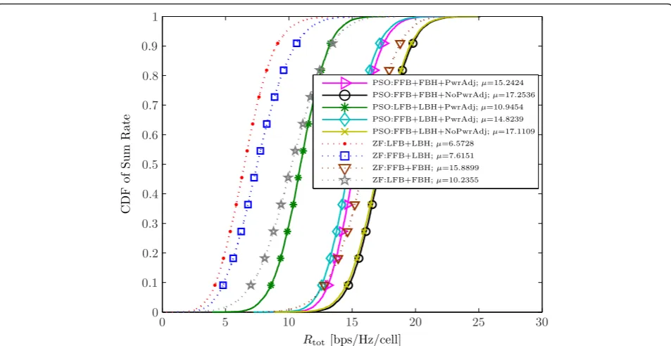
Particle swarm optimization with LFB and LBH performs better than ZF under comparable configurations. The cumulative distribution function (CDF) of the sum rate per cell is shown in Figure 4. The PSO with LFB and LBH performs better than the ZF with LFB and LBH by 66.53% on average. PSO with LFB and LBH also performs better than ZF with FFB and LBH by 43.73% on average. The ZF with FFB and FBH performs better than PSO with FFB and FBH with PwrAdj in every iteration, but PSO with NoPwrAdj shows the best average sum rate compared to the other scenarios considered. This is pri-marily due to the fact that PSO with NoPwrAdj effec-tively uses the BS peak power constraint. The ZF with LFB and FBH (without backhaul load reduction) per-forms better than the ZF with FFB and LBH (with back-haul load reduction). This is similar to the results observed in [9], since the signals received by the UT from BSs outside the active set are seen as desired signals and thus help the UTs to accumulate more energy, but it Table 4 Various precoding configurations

Nos. Precoder Feedback Backhaul Power constraint 6 ZF:LFB + LBH Limited Limited After ZF 7 ZF:FFB + LBH Full Limited After ZF 8 ZF:FFB + FBH Full Full After ZF

(12)

leads to unnecessary backhauling. Due to this minor gain and the undesired additional backhauling, this scenario, ZF with LFB and FBH, is not considered in the following plots.

Alternately, PSO with the objective of maximizing the minimum SINR of the UT was simulated. In the case of LFB and LBH, a 2.1% relative increase in the average sum rate per cell was observed when compared to weighted interference minimization but at the cost of 7.7% relative increase in BSs power consumption and 45% relative increase in interference. As expected inter-ference is greatly affected, hence, weighted interinter-ference minimization is preferred.

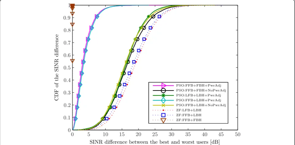
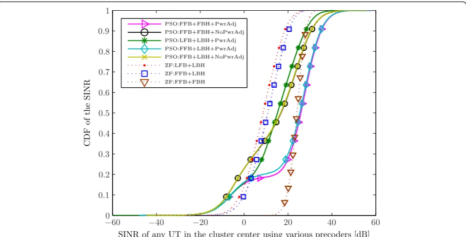
PSO utilizes the available transmit power constraint of Pmax per BS more effectively, and at the same time, it improves the weakest SINR UT. The CDF of the SINR of any UT for various precoding algorithms in any chan-nel realization is shown in Figure 5 with reasonable improvement in the SINR of the weakest UT (the lower part of the CDF). There is an improvement of 2.97% in the average SINR of PSO compared to ZF, under the same conditions of LFB and LBH. We define the SINR difference as [ΔSINR]dB= [SINRm]dB-[SINRm’]dB, where UTm,m ≠m’, experiences the best SINR while UT m’ experiences the best SINR while UT m’experience the worst SINR in agivenchannel realization. The CDF of this SINR difference is shown in Figure 6. With this objective function, where the worst SINR UT is taken care explicitly, the PSO has a much lower variance

compared to the ZF approach. As expected, the ZF approach with FFB and FBH has all the UTs with equal SINR, hence the difference is zero. It is interesting to note that PSO with FFB and LBH with PwrAdj and NoPwrAdj are nearly 15 dB apart in the SINR difference between the best and the worst UT. This is because in the case of NoPwrAdj, applying Equation (3) disfigures the BF weights obtained from the PSO after convergence.

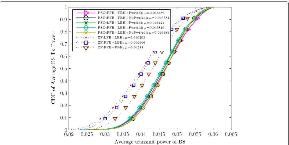
The CDF of the average transmitted power at the BS is shown in Figure 7. The maximum BS transmit power is 0.0603 W, corresponding to a cell-edge SNR of 15 dB. In fact, the PSO keeps the BS power amplifiers on at a higher power, most of the time, which is a desired prop-erty for amplifier efficiency. The power consumption is reduced beforehand with the limited feedback and lim-ited backhauling. PSO uses BS transmit power more effectively when there is a null constraint on the BF (LBH).

It can be seen in Figure 8 that the PSO allows interfer-ence compared to the ZF scenarios. The sum rate is improved even when some interference is remaining in the system. This is similar to the SIN technique in [12], but the SIN technique requires full CSI at the CCN. It is also observed that ZF with FFB and FBH completely removes the interference, but this scheme does not use the available BS transmit power effectively as shown in Figure 7. In the case of PSO, as observed in Figure 8, if LBH is preferred then LFB should also be preferred, as Rtot[bps/Hz/cell]

C

DF

o

fS

um

Ra

te

PSO:FFB+FBH+PwrAdj;µ=15.2424 PSO:FFB+FBH+NoPwrAdj;µ=17.2536 PSO:LFB+LBH+PwrAdj;µ=10.9454 PSO:FFB+LBH+PwrAdj;µ=14.8239 PSO:FFB+LBH+NoPwrAdj;µ=17.1109 ZF:LFB+LBH;µ=6.5728

ZF:FFB+LBH;µ=7.6151 ZF:FFB+FBH;µ=15.8899 ZF:LFB+FBH;µ=10.2355

0 5 10 15 20 25 30

0

0.1

0.2

0.3

0.4

0.5

0.6

0.7

0.8

0.9

1

(13)

PSO with LFB and FFB under PwrAdj shows the same residual interference in the system.

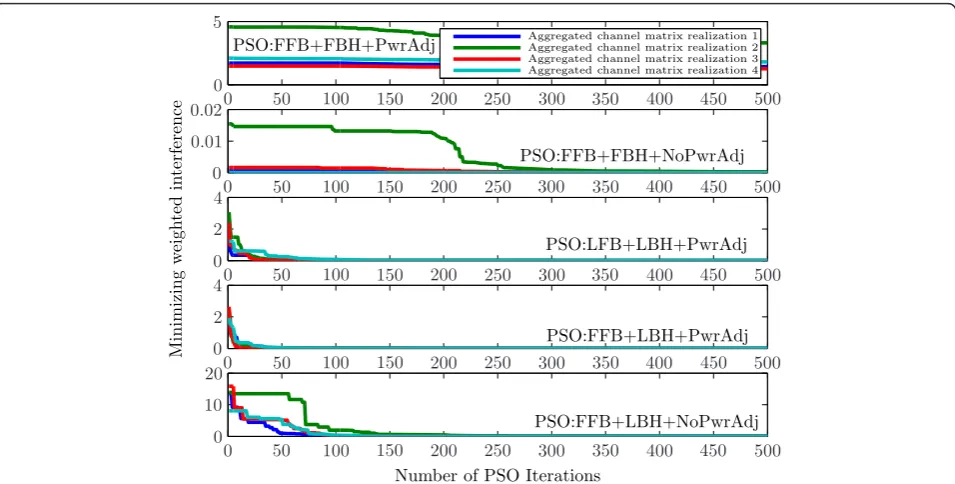
The convergence of the PSO algorithm when evaluat-ing the objective function of weighted interference mini-mization for four randomly chosen aggregated channel matrix realizations is shown in Figure 9 for various

precoder configurations. This objective function con-verges in less than 100 iterations when PSO is applied with LFB and LBH. It can be observed that the number of iterations to find a stable solution is comparatively fast when the number of BF coefficients is small. The conver-gence pattern of FBH is not examined here. This is

SINR of any UT in the cluster center using various precoders [dB]

C

DF

o

f

the

S

INR

PSO:FFB+FBH+PwrAdj PSO:FFB+FBH+NoPwrAdj PSO:LFB+LBH+PwrAdj PSO:FFB+LBH+PwrAdj PSO:FFB+LBH+NoPwrAdj ZF:LFB+LBH

ZF:FFB+LBH ZF:FFB+FBH

−040 −30 −20 −10 0 10 20 30 40 50 60

0.1

0.2

0.3

0.4

0.5

0.6

0.7

0.8

0.9

1

Figure 5CDF of the SINR of any UT for various precoders in any channel realization. PSO with objective function: weighted interference minimization.

SINR diﬀerence between the best and worst users [dB]

C

DF

o

f

the

S

INR

d

iﬀ

erence

0 5 10 15 20 25 30 35 40 45 50

0

0.1

0.2

0.3

0.4

0.5

0.6

0.7

0.8

0.9

1

Figure 6CDF of the SINR difference, [_ΔSINR]dB= [SINRm]dB- [SINRm’]dBbetween the best and the worst UTs in agivenchannel

(14)

because the PSO with FFB and FBH has one of the parti-cles fed with the corresponding solution of PSO with FFB and LBH, during the stochastic initialization phase. This was done to show that the PSO implemented in this arti-cle only finds a stable equilibrium solution and not the global optimum, as increasing the dimensionality of the

problem makes it harder for the PSO, i.e., PSO with unconstrained backhauling, FBH, yielded a slightly poor solution compared to the PSO with constrained back-hauling (LBH), when the objective function was sum rate maximization. To unify our PSO proposal, both objective functions followed the same procedure. This is one of the

Average transmit power of BS

CDF

o

f

A

v

er

a

g

e

BS

Tx

P

o

w

er

PSO:FFB+FBH+PwrAdj;µ=0.046586 PSO:FFB+FBH+NoPwrAdj;µ=0.046584 PSO:LFB+LBH+PwrAdj;µ=0.046121 PSO:FFB+LBH+PwrAdj;µ=0.045819 PSO:FFB+LBH+NoPwrAdj;µ=0.046585 ZF:LFB+LBH;µ=0.040203

ZF:FFB+LBH;µ=0.040906 ZF:FFB+FBH;µ=0.04288

00.02 0.025 0.03 0.035 0.04 0.045 0.05 0.055 0.06 0.065

0.1

0.2

0.3

0.4

0.5

0.6

0.7

0.8

0.9

1

Figure 7CDFs of the average BS transmit power, max = 0.0603 W(17.8 dBm), with cell-edge SNR of 15 dB. PSO with objective function: weighted interference minimization. The value in the legend denotes the mean valueμin a given CDF.

||OﬀDiag(HW_x)||_F

CD

F

o

f

the

Actual

In

terf

erence

0 1 2 3 4 5 6 7 8 9

0.55

0.6

0.65

0.7

0.75

0.8

0.85

0.9

(15)

main reasons why the convergence curves of PSO with FBH remain relatively flat.

Based on the analysis in Section 3.4 and on the prior experience, the number of BF coefficients carried by a particle decreases with the sparsity of the aggregated channel matrix. With LBH, the PSO converges faster than the case when there is FBH. Reference to Figure 9 could be unfair, due to the reason cited earlier that the solution of PSO with LBH is fed to one of the particles in the case of FBH. If this is not performed, then the faster convergence of the PSO is observed (not shown here).

5.2 Objective function: sum rate maximization

When the objective of the PSO is to maximize the sum rate, the maximization is indirectly related to the parti-cles in the PSO carrying the BF weights via the logarithm. This objective is very sensitive to the power adjustment performed after the PSO algorithm has converged. The CDF of the SINR of any UT is shown in Figure 10. It can be observed that the ambition of improving only the sum rate of the system penalizes the weak SINR UTs.

5.3 Gershgorin’s circles

In the complex plane, Figure 11 shows the circumference of the Gershgorin’s discs for various precoders, with the objective of the PSO being weighted interference minimi-zation. This figure is plotted for a given reference SINR value of the PSO with FFB and FBH. The receiver noise is assumed to be uniform across all the UTs, and SINR is plotted instead of SIR. The green‘+’refers to the elements

in the diagonal of the matrixD= diag(HW),representing the Gershgorin’s estimate of the eigen value. The absolute sum of the off diagonal elements forms the radius of the blue Gershgorin’s circles for that eigen value and it is plotted with the green‘+’as its center. The blue bigger cir-cles show the multiuser interference remaining in the sys-tem for a given precoder. The actual eigen values are plotted in red squares as‘□’. It can be seen that the PSO gives more freedom for the eigen values to move around in the complex plane, thereby increasing the power trans-mitted to the UTs. ZF with FFB and FBH completely removes the interference and hence the blue multiuser interference circles are not visible. The ZF approach aims to serve all the UTs equally and hence their actual eigen values are closer together.

It is interesting to note that for the PSO with LFB and LBH, the actual eigen values map closely to the esti-mated Gershgorin’s eigen values, unlike the ZF with LFB and LBH. From an interference point of view, hav-ing concentric circles helps containhav-ing the interference within the largest circle. ZF with LFB and LBH shows this attribute.

6 Conclusions

In this work, a particle swarm stochastic optimization algorithm has been proposed in a partial JP framework to design the precoding weights for efficient backhauling, achieving a backhaul reduction proportional to the reduc-tion in the CSI feedback. In this context, two objective functions have been considered, a weighted interference

Aggregated channel matrix realization 1 Aggregated channel matrix realization 2 Aggregated channel matrix realization 3 Aggregated channel matrix realization 4

Minimizing

w

eig

h

ted

in

ter

ference

Number of PSO Iterations

PSO:FFB+FBH+NoPwrAdj

PSO:LFB+LBH+PwrAdj

PSO:FFB+LBH+PwrAdj

PSO:FFB+LBH+NoPwrAdj PSO:FFB+FBH+PwrAdj

0 50 100 150 200 250 300 350 400 450 500

0 10 20 0 2 4 0 2 4 0

0.01

0.02

0 5

(16)

minimization and a sum rate maximization. In the pro-posed weighted interference minimization, the SINR of the weakest UT is iteratively improved, in addition to the interference minimization. With the limited feedback and limited backhaul constraints, and the weighted interfer-ence minimization as the objective function, the average sum rate per cell of the UTs is improved by 66.53% with respect to a ZF precoder. The particle swarm based pre-coder allows some multiuser interference to remain in the system, still improving the sum rate, and it uses the BS transmit power more effectively.

With recent developments in swarm intelligence, the complexity and the feasibility can be improved to achieve a faster and a more robust particle swarm algorithm. There is potential for improving the PSO algorithm with capabilities to perform global search, such as random PSO, which should improve the already promising results presented in this article.

Algorithm 1 Active set thresholding for limited feedback based on [7]

1: Choose:threshold= 10 dB 2:foreach UTdo

3: Measure the channel gain from all BSs 4: bestLink= max{channel strength from all BSs} 5: if(bestLink - otherLink)≤thresholdthen

6: UT feed backs the CSI ofotherLink

7: CCN marks this link asactive

8: else

9: Feedback load reduction:

10: UT does not feed back theotherLink

11: CCN marks this link asinactive

12: end if

13: UT feeds back thebestLink 14: CCN marks this link asactive 15:end for

Algorithm 2 Pseudocode for obtaining the BF via PSO. Steps 3 to 5 are only mentioned for

illustration and can be avoided prior to initialization

1:Initialization:

2: Determine the number of non-zero coefficients n needed in the BF matrix, _W

3: Map the BF to the particle:

4: X(i,j)← {W(l,m)},l∈ {1, ...,KNT},m∈ {1, ...,M} 5: X(i,j+ 1)← {W(l,m)}

6: Stochastically initialize particles with BF coefficients: 7: xmax= 1/ max|H(i,j)|

8: xmin= -xmax

9: Position:X(i,j) =xmin+r · (xmax-xmin)

10: Velocity: V(i,j) = 1 t

−(xmax−xmin)

2 +s·(xmax−xmin)

11:whileTermination Criteriondo

12: fortheith particle in the swarmdo

13: Demap the variables in a particle to form the BF matrix

SINR of any UT in the cluster center using various precoders [dB]

C

DF

o

f

the

S

INR

−060 −40 −20 0 20 40 60

0.1

0.2

0.3

0.4

0.5

0.6

0.7

0.8

0.9

1

(17)

14: W(l,m)← {X(i,j)}+ i· {X(i,j+ 1)} 15: Evaluate the objective functionf(X(i, :)) 16: Store:

17: iff(X(i,:)) <fpb(X(i,:))then

18: Particles’Best:Xpb(i,:)¬X(i,:) 19: end if

20: iff(X(i,:)) <fsb(X(i,:))then

21: Swarm’s Best:xsb ¬X(i,:) 22: _Wsb₍_l_,_m₎_{← {}_xsb₍_j₎_}_{+ i.}_{_xsb₍_j_{+ 1)}_}

23: end if

24: end for

25: for Each particle in the swarm with BF coeffi-cientsdo

26: Update:

27: Velocity: V(i,j)←w·V(i,j) +c1·p·

Xpb₍_i_,_j₎₋_X₍_i_,_j₎ t

+c2·q·X sb₍_j₎₋_X₍_i_,_j₎

t 28: Restrict velocity:|V(i,j)| < vmax

29: Position:X(i,j)¬ X(i,j) +V(i,j) ·Δt 30: end for

31: w¬w·b

0.5

1 x 10

-16

ZF:FFB+FBH

(18)

Abbreviations

BF: beamformer (-ing); bps: bits per second; BS(s): base station(s); CCN: central coordination node; CDF: cumulative distribution function; CJP: centralized joint processing; CoMP: Coordinate MultiPoint (transmission); CSI: channel state information; FBH: Full BackHauling; FFB: Full FeedBack; JP: joint processing; LBH: Limited BackHauling; LFB: Limited FeedBack; MAC: medium access control; MU-MIMO: MultiUser Multiple Input Multiple Output; NoPwrAdj: no power adjustment; PJP: partial joint processing; PHY: physical; PwrAdj: power adjustment; PSO: particle swarm optimization; SIR: signal to interference ratio; SINR: signal to interference plus noise ratio; SNR: signal to noise ratio; SIN: soft interference nulling; UT(s): user terminal(s); ZF: zero forcing.

Acknowledgements

The authors would like to thank the reviewers for their critical comments that greatly improved the article. This study has been partly supported by the Swedish Research Council, within the project 621-2009-4555 Dynamic Multipoint Wireless Transmission. This study is also been supported by The Swedish Agency for Innovation Systems (VINNOVA) and by the EU FP7 project INFSO-ICT-247223 ARTIST4G. C. Botella’s work has been supported by the Spanish MEC Grants CONSOLIDER-INGENIO 2010 CSD2008-00010

“COMONSENS”and COSIMA TEC2010-19545-C04-01. The authors would also like to acknowledge the members of the VR meetings, in particular Jingya Li and Agisilaos Papadogiannis for the valuable discussions. Thanks to Bhavishya Goel for the fruitful discussions on complexity. The computations were performed on C3_{SE computing resources.}

Author details

1_{Department of Signals and Systems, Chalmers University of Technology, 412} 96 Gothenburg, Sweden2Institute of Robotics and Information &

Communication Technologies (IRTIC), Universitat de València, València, Spain

Competing interests

The authors declare that they have no competing interests.

Received: 30 June 2011 Accepted: 29 May 2012 Published: 29 May 2012

References

1. 3GPP TR 36.814-900, 3rd Generation Partnership Project; Technical specification group radio access network; Further advancements for E-UTRA physical layer aspects (Release 9) (2010)

2. MK Karakayali, GJ Foschini, RA Valenzuela, Network coordination for spectrally efficient communications in cellular systems. IEEE Wirel Commun.

13(4), 56_–61 (2006). doi:10.1109/MWC.2006.1678166

3. D Gesbert, S Hanly, H Huang, SS Shitz, O Simeone, Wei Yu, Multi-cell MIMO cooperative networks: a new look at interference. IEEE J Sel Areas Commun.

28(9), 1380–1408 (2010)

4. A Papadogiannis, E Hardouin, D Gesbert, Decentralising multi-cell cooperative processing: a novel robust framework. EURASIP J Wirel Commun Netw 1–10 (2009). Article ID 890685

5. P Marsch, G Fettweis, A framework for optimizing the downlink of distributed antenna systems under a constrained backhaul. inProc European Wireless Conference,Paris, France 1_–5 (2007)

6. P Marsch, G Fettweis, On multicell cooperative transmission in backhaul-constrained cellular systems. Ann Telecommun.63(5), 253_–269 (2008). doi:10.1007/s12243-008-0028-3

7. C Botella, T Svensson, X Xu, H Zhang, On the performance of joint processing schemes over the cluster area. inProc IEEE Vehicular Technology Conference, Taipei, Taiwan 1–5 (2010)

8. A Papadogiannis, H Bang, D Gesbert, E Hardouin, Downlink overhead reduction for multicell cooperative processing enabled wireless networks. in IEEE Personal, Indoor and Mobile Radio Communications, Cannes, France 1–5 (2008)

9. A Papadogiannis, HJ Bang, D Gesbert, E Hardouin, Efficient selective feedback design for multicell cooperative networks. IEEE Trans Veh Technol.

60(1), 196_–205 (2011)

10. F Boccardi, H Huang, A Alexiou, Network MIMO with reduced backhaul requirements by MAC coordination. inProc IEEE Asilomar Conference on Signals, Systems and Computers, Pacific Grove 1125–1129 (2008)

11. J Zhang, R Chen, JG Andrews, A Ghosh, RW Heath, Networked MIMO with clustered linear precoding. IEEE Trans Wirel Commun.8(4), 1910–1921 (2009)

12. CTK Ng, H Huang, Linear precoding in cooperative MIMO cellular networks with limited coordination clusters. IEEE J Sel Areas Commun.28(9), 1446_–1454 (2010)

13. TR Lakshmana, C Botella, T Svensson, X Xu, J Li, X Chen, Partial joint processing for frequency selective channels. inProc IEEE Vehicular Technology Conference, Ottawa, Canada 1–5 (2010)

14. X Wei, T Weber, A Kuhne, A Klein, Joint transmission with imperfect partial channel state information. inProc IEEE Vehicular Technology Conference, Barcelona, Spain 1–5 (2009)

15. S Fang, G Wu, S-Q Li, Optimal multiuser MIMO linear precoding with LMMSE receiver. EURASIP J Wirel Commun Netw 1–10 (2009). Article ID 197682

16. Y Hei, X Li, K Yi, H Yang, Novel scheduling strategy for downlink multiuser MIMO system: particle swarm optimization. Sci China F.52(12), 2279_–2289 (2009). doi:10.1007/s11432-009-0212-8

17. C Knievel, PA Hoeher, A Tyrrell, G Auer, Particle swarm enhanced graph-based channel estimation for MIMO-OFDM. inProc IEEE Vehicular Technology Conference, Budapest, Hungary 1–5 (2011)

18. P Marsch, G Fettweis, On downlink network MIMO under a constrained backhaul and imperfect channel knowledge. inGlobal Telecommunications Conference, California, USA 1_–6 (2009)

19. Q Spencer, A Swindlehurst, M Haardt, Zero-forcing methods for downlink spatial multiplexing in multiuser MIMO channels. IEEE Trans Signal Process.

52(2), 461–471 (2004). doi:10.1109/TSP.2003.821107

20. H Zhang, H Dai, Cochannel interference mitigation and cooperative processing in downlink multicell multiuser MIMO networks. EURASIP J Wirel Commun Netw.2, 222–235 (2004)

21. TR Lakshmana, C Botella, T Svensson, Partial Joint Processing with Efficient Back-hauling in Coordinated MultiPoint Networks. inProc IEEE Vehicular Technology Conference, Yokohama, Japan 1–5 (2012)

22. J Kennedy, RC Eberhart, Particle swarm optimization. inProc IEEE International Conference on Neural Networks, Perth, Australia 1942_–1948 (1995)

23. AP Engelbrecht,Fundamentals of Computational Swarm IntelligenceJohn Wiley 171–172 (2005)

24. YH Shi, RC Eberhart, Parameter selection in particle swarm optimization. in The 7th Annual Conference on Evolutionary Programming, San Diego, USA 591–601 (1998)

25. C-B Chae, S-H Kim, RW Heath, Network coordinated beamforming for cell-boundary users: linear and nonlinear approaches. IEEE J Sel Top Signal Process.3(6), 1094_–1105 (2009)

26. CB Peel, BM Hochwald, AL Swindlehurst, A vector-perturbation technique for near-capacity multiantenna multiuser communication-part I: channel inversion and regularization. IEEE Trans Commun.53(1), 195–202 (2005). doi:10.1109/TCOMM.2004.840638

27. RA Horn, CR Johnson,Matrix Analysis, (Cambridge University Press, Cambridge, 1985), pp. 344–347

28. 3GPP TR 36.942-a20, 3rd Generation Partnership Project; Technical specification group radio access network; Evolved universal terrestrial radio access; Radio frequency system scenarios (Release 10) (2011)

29. ARTIST4G D1.2, Innovative advanced signal processing algorithms for interference avoidance, ARTIST4G technical deliverable, p. 84 https://ict-artist4g.eu/projet/work-packages/wp1/documents/d1.2/d1.2.pdf. Accessed 17 June 2010

doi:10.1186/1687-1499-2012-182