R E S E A R C H
Open Access
Analysis of an
SIRS
epidemic model with
time delay on heterogeneous network
Qiming Liu
1*, Meici Sun
1and Tao Li
1,2*Correspondence:
lqmmath@163.com
1Shijiazhuang Campus, Arm
Engineering University, Shijiazhuang, 050003, China Full list of author information is available at the end of the article
Abstract
We discuss a novel epidemicSIRSmodel with time delay on a scale-free network in this paper. We give an equation of the basic reproductive numberR0for the model and prove that the disease-free equilibrium is globally attractive and that the disease dies out whenR0< 1, while the disease is uniformly persistent whenR0> 1. In addition, by using a suitable Lyapunov function, we establish a set of sufficient conditions on the global attractiveness of the endemic equilibrium of the system.
Keywords: epidemic spreading; scale-free network; basic reproductive number; global attractiveness; time delay
1 Introduction
Following both the seminal work on small-world network phenomena by Watts and Stro-gatz [] and the scale-free network, in which the probability ofp(k) for any node withk links to other nodes is distributed according to the power lawp(k) =Ck–γ( <γ≤),
sug-gested by Barabási and Albert [], the spreading of an epidemic disease on heterogeneous networks,i.e., scale-free networks, has been studied by many researchers [–].
Realistic epidemic models should include some past states of the system, and time de-lay pde-lays an important role in the spreading process of the epidemic. For instance, it can simulate the incubation period of the infectious disease, the infectious period of patients, and the immunity period of recovery of the disease with time delay [, ]. However, only little attention has been given to the epidemic models with time delays on heteroge-neous networks. Liu and Xu presented a functional differential equationSEIRSepidemic model, in which time delay represents the latent period and the immune period []. Liu and Denget al.discussed a functional differential equationSISmodel, in which time de-lay represents the average infectious period [], obtained the basic reproduction number, and discussed the persistence of the disease. Wang and Wanget al.presented a functional differential equationSIRmodel, in which time delay represents the incubation period, and discussed the global stability of equilibria of the system []. Kang and Fu also established a functional differential equationSISmodel with an infective vector and analyzed the global stability of the endemic equilibrium, the disease-free equilibrium [], and so on.
Considering the fact that the immune individual may become the susceptible individual, Chen and Sun discussed anSIRSepidemic model without delay []. In [], Wang and Wanget al.presented a delayedSIRmodel, in which time delay represents the incubation
period during which the infectious agents develop in the vector, and discussed the global stability of equilibria of the system. Motivated by the work of Chen [] and Wang [], we will present a novel functional differential equationSIRSmodel in which time delay rep-resents the incubation period of an infective vector to investigate the epidemic spreading on a heterogeneous network.
Assuming the size of the network is a constantNduring the period of epidemic spread-ing, we also suppose that the degree of each node is time-invariant andp(k) denotes the degree distribution of the network. LetSk(t),Ik(t), and Rk(t) be the relative density of susceptible nodes, infected nodes, and recovered nodes of connectivityk at timet, re-spectively, wherek=m,m+ , . . . ,n, in whichmandnare the minimum and maximum degree in network topology, respectively. Since the number of total nodes with degreek is a constantp(k)Nduring the period of epidemic spreading, the following normalization conditions hold:
Sk(t) +Ik(t) +Rk(t) = , k=m,m+ , . . . ,n.
In propagation processes of the epidemic via a vector (such as the mosquito), when a sus-ceptible vector is infected by an infected one, there is a delayτduring which the infectious agents develop in the vector and the infected vector becomes itself infectious after the de-lay. At the same time, the vector’s usual activities are in a limited range, and the vector population size is large enough such that at any timeta number of the infectious vector population in the vicinity of the infected nodes with degreek(k=m,m+ , . . . ,n) at any timetis simply proportional to the number of the infected nodes with degreek. The dy-namical equations for the densitySk(t),Ik(t), andRk(t), at the mean-field level, satisfy the following set of functional differential equations whent> [, , ]:
˙
Sk(t) = –λ(k)Sk(t)(t–τ) –δSk(t) +μRk(t), ˙
Ik(t) =λ(k)Sk(t)(t–τ) –rIk(t),
˙
Rk(t) =rIk(t) –μRk(t) +δSk(t),
()
whereλ(k) is a transmission coefficient of the disease between the susceptible nodes and infected nodes andris the recovery rate from the infected nodes to the recovered nodes because the infected nodes (patients) are cured.δis the removal rate from the susceptible nodes to the recovered nodes because the susceptible nodes acquire temporary immunity. μis the removal rate from the recovered nodes to the susceptible nodes because the re-covered nodes lose temporary immunity. The dynamics ofngroups ofSIRSsubsystems are coupled through the function(t), which represents the probability that any given link points to an infected node at timet. Considering the uncorrelated network [, ], we have
(t) = k
n
k=m
ϕ(k)p(k)Ik(t), ()
≤α< ,a> ,b≥ []. With different parameters,ϕ(k) can be divided into different cases, such asϕ(k) =k[] whenα= ,b= , anda= ;ϕ(k) =A[] whena=A,α= , and b= ;ϕ(k) =kα [] whena= andb= . Specially, ifb= ,ϕ(k) will become gradually
saturated as degreekincreases,i.e.,limk→∞ϕ(k) =b/a. The initial conditions of system () are the following:
Sk(θ) =ζk(θ), Ik(θ) =ψk(θ),
Rk(θ) =φk(θ), θ∈[–τ, ],k=m,m+ , . . . ,n,
()
whereω= (ζm(θ),ψm(θ),φm(θ), . . . ,ζn(θ),ψn(θ),φn(θ))∈Care nonnegative continuous on [–τ, ] andζk() > ,ψk() > forθ= .Cdenotes the Banach spaceC([–τ, ],R(n–m+)) with the norm
ω=
n
i=m ζi(θ)
τ +ψi(θ)
τ+φi(θ)
τ
/ ,
where
f(θ)τ= sup
–τ≤θ≤
f(θ).
It is well known, by the fundamental theory of functional differential equations [], that system () has a unique solution (Sm(t), . . . ,Sn(t),Im(t), . . . ,In(t),Rm(t), . . . ,Rn(t)) satisfying the initial conditions (). It is easy to show that all solutions of system () with initial con-ditions () are defined on [, +∞) due to the boundedness ofSk,Ik, andRk. In addition, using similar arguments as in [], it is easy to show that all solutions of system () with initial conditions () remain positive for allt≥.
The rest of this paper is organized as follows. The dynamical behaviors of theSIRSmodel are discussed in Section . Numerical simulations and discussions are given to demon-strate the main results in Section . Finally, the main conclusions of this work are summa-rized in Section .
2 Dynamical behaviors of the model
Note thatSk(t) +Ik(t) +Rk(t) = . If we discuss the dynamical behaviors of system (), we only discuss the following equivalent system of model ():
˙
Sk(t) = –λ(k)Sk(t)(t–τ) –δSk(t) +μ –Sk(t) –Ik(t), ˙
Ik(t) =λ(k)Sk(t)(t–τ) –rIk(t).
()
Denote
R=
μ (μ+δ)r
λ(k)ϕ(k)
k , ()
wheref(k)=kf(k)p(k), in whichf(k) is a function.
Note that we obtain from the first equation of system () the following equation:
˙
By the standard comparison theorem in the theory of differential equations, we have
lim
t→+∞supSk(t)≤μ/(μ+δ). ()
Hence we know
D= (Sm,Im, . . . ,Sn,In)∈R+(n–m+) <Sk,Ik,Sk+Ik≤, <Sk≤
μ μ+δ
is positively invariant with respect to system (), and every forward orbit inR(+n–m+)
even-tually entersD.
Theorem System()always has a disease-free equilibrium E(μμ+δ, . . . , μ
μ+δ, , . . . , ).
Sys-tem()has a unique endemic equilibrium E∗(Sm∗,Sm∗+, . . . ,S∗n,Im∗,Im∗+, . . . ,In∗)when R> .
Proof Obviously, the disease-free equilibriumEof system () always exists. Now we
dis-cuss the existence of the endemic equilibrium of system (). Note that the equilibriumE∗ should satisfy
–λ(k)S∗k∗–δSk∗+μ –S∗k–Ik∗= ,
λ(k)S∗k∗–rIk∗= ,
()
where
∗= k
k
ϕ(k)p(k)Ik∗. ()
From (), we obtain
Ik∗= λ(k)μ ∗
(μ+δ)r+λ(k)(r+μ)∗. ()
Substituting this into (), we obtain the self-consistency equality
∗= k
k
ϕ(k)p(k) λ(k)μ ∗
(μ+δ)r+λ(k)(r+μ)∗, ()
similar to the proof of Theorem in []. Equation () has a unique positive solution whenR> and consequently, system () has a unique endemic equilibriumE∗since ()
and () hold.
Remark We know that the basic reproductive number for system () isR. Ifϕ(k) =k
andτ= , system () reduces to theSIRSmodel (.) without delay in [], andRin this
paper consists/coincides with one of the model in [].
Theorem If R< ,the disease-free equilibrium Eof system()is globally attractive.
Consider the following Lyapunov function:
V(t) =
(t) +η
t
t–τ
(μ)dμ,
whereηis a constant to be determined.
Calculating the derivative ofV(t) along the solution of (), we get
˙
V(t)()=(t)
k
k
φ(k)p(k)λ(k)Sk(t)(t–τ) –rIk(t)+η(t) –η(t–τ).
Note that <Sk(t)≤μ/(μ+δ) according to the positive invariance ofD. We have
˙
V(t)()≤(t)
k
k
φ(k)p(k)
λ(k) μ
μ+δ(t–τ) –rIk(t)
+η(t) –η(t–τ)
=(t)(t–τ) μ μ+δ
λ(k)φ(k)
k –r
(t) +η(t) –η(t–τ)
≤
(t) +(t–τ) μ μ+δ
λ(k)φ(k)
k –r
(t) +η(t) –η(t–τ).
Letη=μμ+δλ(kk)ϕ(k). We have
˙ V(t)()≤
μ μ+δ
λ(k)φ(k) k –r
(t) =r(R– )(t).
ThusV˙(t)|()≤ whenR< andV˙(t)|()= if and only if= . Note that the fact that
= means thatIk= . Moreover,limt→+∞Sk(t) =μ/(μ+δ), the largest invariant set ofV˙(t)|()= is a singletonE. Therefore, by the LaSalle invariance principle (see [,
Chapter , Theorem .]), the disease-free equilibriumEis globally attractive.
Lemma ([]) Consider the following equation:
˙
x(t) =ax(t–τ) –ax(t),
where a,a,τ> ;x(t) > for–τ≤t≤.We have (i) ifa<a,thenlimt→+∞x(t) = ,
(ii) ifa>a,thenlimt→+∞x(t) = +∞.
Theorem For system(), if R> , the disease-free equilibrium E is unstable, and
the disease is uniformly persistent, i.e., there exists a positive constant such that limt→+∞infIk(t)≥,k=m,m+ , . . . ,n.
Proof Denote
X=(S¯,ψ¯) :ψk(θ)≥, for allθ∈[–τ, ],k=m,m+ , . . . ,n
,
X=(S¯,ψ¯) :ψk(θ) > , for someθ∈[–τ, ],k=m,m+ , . . . ,n
Consequently, we have
∂X=X/X=(S¯,ψ¯) :ψi(θ) = , for allθ∈[–τ, ],i∈ {m,m+ , . . . ,n}
,
where (S¯,ψ¯) = (Sm,Sm+, . . . ,Sn,ψm,ψm+, . . . ,ψn).
Let (Sm(t),Im(t), . . . ,Sn,In(t)) = (Sm(t,ω),Im(t,ω), . . . ,Sn(t,ω),In(t,ω)) be the solution of () with initial functionω= (ζm(θ),ψm(θ), . . . ,ψn(θ),φn(θ)) and
T(t)(ω)(θ) =Sm(t+θ,ω),Im(t+θ,ω), . . . ,Sn(t+θ,ω),In(t+θ,ω), θ∈[–τ, ].
Obviously,XandXare positively invariant sets forT(t).T(t) is completely continuous
fort> . Also, it follows from <Sk(t),Ik(t)≤ fort> thatT(t) is point-dissipative.E
is the unique equilibrium of system () on∂Xand it is globally stable on∂X,A˜
∂={E},
andEis isolated and acyclic. Finally, the proof will be complete if we proveWs(E)∩X=
∅, whereWs(E
) is the stable manifold ofE. Suppose it is not true. Then there exists a
solution (S¯,¯I) inXsuch that
lim t→+∞
Sk(t),Ik(t)=
μ μ+δ,
, k=m,m+ , . . . ,n.
SinceR> , we may choose <η< such that (λ(kμ)η(–+μη+)δ)rλ(kk)ϕ(k)> . At the same time,
there exists aT> such that ≤Ik(t) <ηfort>Tdue tolimt→+∞infIk(t) = . Whent>T, we obtain from the first equation of system ()
˙
Sk(t) > –λ(k)Skη+μ –Sk(t) –η–δSk(t)
=μ( –η) –λ(k)η+μ+δSk(t).
Hence there exists aT>Tsuch that the following equality holds whent>T:
Sk(t)≥ μ( –η)
λ(k)η+μ+δ. ()
Fort>T, we have from () and ()
˙ (t) =
k
k
ϕ(k)p(k)Ik˙(t)
= k
k
ϕ(k)p(k)λ(k)Sk(t)(t–τ) –rIk(t)
≥ μ( –η) λ(k)η+μ+δ
λ(k)ϕ(k)
k (t–τ) –r(t).
Note that (λ(kμ)(–η+μη+)δ)rλ(kk)ϕ(k) > . It follows that λ(μk)(–η+ημ)+δλ(kk)ϕ(k) >r. Hence we deduce from () thatlimt→+∞(t) = +∞according to Lemma , contradictinglimt→+∞(t) = due to limt→+∞Ik(t) = . Hence limt→+∞inf(t)= . Moreover, there exists a k ∈
{m,m + , . . . ,n} such that limt→+∞infIk(t)= , contradicting limt→+∞infIk(t) = ,
k=m,m+ , . . . ,n.
limt→+∞infSk(t)≥. The disease-free equilibriumEis unstable accordingly. This
com-pletes the proof.
Furthermore, we obtain the following Theorem about the global attractiveness of the endemic equilibriumE∗of system () by constructing a suitable Lyapunov function.
Theorem If R> ,δ<r,and Ik∗<μ/(μ+δ)(δ/r),k=m,m+ , . . . ,n,then the endemic equilibrium E∗of system()is globally attractive.
Proof For convenience, we still discuss system ().
In accordance with () andSk(t) +Ik(t) +Rk(t) = ,k=m,m+ , . . . ,n, we know
˜
D= (Sm,Im,Rm, . . . ,Sn,In,Rn)∈R(+n–m+)
<Sk,Ik,Rk,Sk+Ik+Rn= , <Sk≤ μ μ+δ
()
is positively invariant with respect to system (), and every forward orbit inR(+n–m+)
even-tually entersD˜.
Thus we just need to discuss the global attractiveness of system () inD˜.
DenoteR∗k= –Sk∗–Ik∗. ThenE∗(Sm∗,Im∗,R∗m,S∗m+,Im∗+,R∗m+, . . . ,S∗n,In∗,R∗n, ) is the endemic equilibrium of system (). System () may be rewritten as the following system:
˙ Sk(t) = –
n
l=m
βklSk(t)Il(t–τ) –δSk(t) +μRk(t),
˙ Ik(t) =
n
l=m
βklSk(t)Il(t–τ) –rIk(t),
˙
Rk(t) =r– (μ+r)Rk(t) – (r–δ)Sk(t),
()
whereβkl=λ(l)ϕk(l)p(l),l=m,m+ , . . . ,n.
Note that the endemic equilibrium of system () satisfies
– n
l=m
βklS∗kIl∗–δS∗k+μR∗k= ,
n
l=m
βklSk∗Il∗=rIk∗,
(μ+r)R∗k+ (δ–r)S∗k=r.
()
We have from () and () that
˙ Sk(t) = –
n
l=m
βklSk(t)Il(t–τ) + n
l=m
βklS∗kIl∗–δ(Sk–S∗k) +μRk–R∗k,
˙ Ik(t) =
n
l=m
βklSk(t)Il(t–τ) – n
l=m βkl
S∗kIl∗ Ik∗ Ik(t),
˙
Rk(t) = –(μ+r)Rk–R∗k+ (δ–r)Sk–S∗k.
Let us consider
Calculating the derivative ofVk(t) along a solution of (), we get
Since Ik∗<δ/(μ+δ)(μ/r), we take ε=δ/(μ+δ) –Ik∗r/μ> . It follows from () that
is irreducible, so the following matrix is irreducible:
B=
Define a Lyapunov function as follows:
Moreover,V˙(t)|()= if and only ifSk=Sk∗,Ik=Ik∗, andRk=R∗k. Therefore, by the LaSalle invariance principle (see [, Chapter , Theorem .]), the endemic equilibriumE∗ is globally attractive whenR> ,δ<randIk∗<μ/(μ+δ)(δ/r),k=m,m+ , . . . ,n. The proof
is completed.
3 Numerical simulations and discussions
The basic reproductive number for system () (or ()) is
R=
μ (μ+δ)r
λ(k)ϕ(k)
k . ()
The equilibrium E is globally attractive and the infection eventually disappears when
R< . The infection will always exist whenR> . Note thatRis irrelative toτ.
Now we present numerical simulations to demonstrate the above mentioned theorems. Note that we obtain the equilibria from system (). The simulations are based on system () and a scale-free network in which the degree distribution isp(k) =Ck–γandCsatisfies
n
k=mp(k) = . Assuming the network is finite, the maximum connectivitynof any node is related to the network age, measured as the number of nodesN[, ]. We have
n=mN/(γ–). ()
Letn= andm= be suitable assumptions. Letφ(k) =akα/( +bkα) in whicha= .,
α= .,b= ., andλ(k) =λk. The initial functions areIk(s) = .,k= , , , , and Ik= ,k= , , , fors∈[,τ].
Denote
I(t) = k
p(k)Ik(t).
Obviously,I(t) is the relative average density of the infected nodes.
Case : Letλ= .,r= .,δ= .,μ= .,γ = ., andτ= . We obtain from () thatR= . < . Figure shows the dynamic behaviors of system (). The numerical
simulation shows thatlimt→+∞I(t) = . It follows thatlimt→+∞Ik(t) = and the infection eventually disappears. The numerical result is consistent with Theorem .
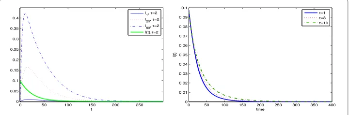
Case : Letλ= .,r= .,δ= .,μ= .,γ = .,τ = , andδ<r. We obtain from () that R= . > andmaxIk∗= . <μ/(μ+δ)(δ/r) = .. Figure
Figure 2 Dynamical behaviors of system (4) withR0= 1.4596.
Figure 3 Dynamical behaviors of system (4) withτ= 2 andR0= 1.5793.
shows the dynamic behaviors of system (). The average densitiesIk(t) andI(t) converge to a positive constant ast→+∞and the infection is uniformly persistent. The numerical result is consistent with Theorems and .
Although the time delayτhas no effects on both the spreading threshold and the density of infected nodes at the stationary state according to () and (), we find that the delayτ has much impact on the densityI(t) of the infected nodes; the slower the relative density of infected nodes converges to the stationary state, the largerτgets. Thus the delay cannot be ignored. The numerical simulations in Figure and Figure verify it.
Moreover, letλ= .,r= .,δ= .,μ= .,γ = .,τ= , andδ<r. We obtain from () thatR= . > butIk∗≥μ/(μ+δ)(δ/r) = ., ≤k≤. Figure
shows the dynamic behaviors of system (). The parameters of system () do not satisfy Theorem , but the relative densityIk(t) and the relative average densityI(t) still converge to a positive constant ast→+∞. At the same time, no Hopf bifurcation occurs, so The-orem has room for improvement.
4 Conclusions
AnSIRSmodel with time delay on a scale-free network has been proposed, in which time delay describes the incubation period of the infective vector. We obtained the basic re-production numberR, which is irrelative toτ. The disease-free equilibrium is globally
attractive and infection may disappear whenR< , while the infection is uniformly
per-sistent whenR> . Moreover, the endemic equilibrium is globally attractive ifR> ,δ<r,
that the endemic equilibrium is still globally attractive even ifδ<randI∗k<μ/(μ+δ)(δ/r), k=m,m+ , . . . ,ndo not hold whenR> . Therefore, improvement of the sufficient
con-dition in Theorem on the global attractiveness of the endemic equilibrium of system () is an interesting but challenging problem.
Acknowledgements
The authors are very grateful to the anonymous referees for their valuable suggestions, which greatly led to significant improvement of the original manuscript. This research was supported by the Hebei Provincial Natural Science Foundation of China under Grant No. A2016506002 and the Innovation Foundation of Shijiazhuang Mechanical Engineering College under Grant No. YSCX1201.
Competing interests
The authors declare that they have no competing interests.
Authors’ contributions
All authors contributed to the expression of the model and the discussion of results. They read and approved the final manuscript.
Author details
1Shijiazhuang Campus, Arm Engineering University, Shijiazhuang, 050003, China.2The 260th Hospital of PLA,
Shijiazhuang, 050041, China.
Publisher’s Note
Springer Nature remains neutral with regard to jurisdictional claims in published maps and institutional affiliations.
Received: 15 June 2016 Accepted: 19 September 2017
References
1. Watts, DJ, Strogatz, SH: Collective dynamics of small world networks. Nature393, 440-442 (1998) 2. Barabási, AL, Alber, R: Emergence of scaling in random networks. Science286, 509-512 (1999)
3. Pastor-Satorras, R, Vespignani, A: Epidemic dynamics in finite size scale-free networks. Phys. Rev. E65, Article ID 035108 (2002)
4. Balthrop, J, Forrest, S, Newman, M, Williamson, M: Technological networks and the spread of computer viruses. Science304, 527-529 (2004)
5. Yang, R, Wang, B, Ren, J, Bai, W, Shi, Z, Wang, W, Zhou, T: Epidemic spreading on heterogeneous networks with identical infectivity. Phys. Lett. A364, 189-193 (2007)
6. Cheng, X, Liu, X, Chen, Z, Yuan, Z: Spreading behavior of SIS model with non-uniform transmission on scale-free networks. J. China Univ. Post Telecommun.16, 27-31 (2009)
7. Zhang, H, Fu, X: Spreading of epidemics on scale-free networks with nonlinear infectivity. Nonlinear Anal.70, 3273-3278 (2009)
8. Li, K, Small, M, Zhang, H, Fu, X: Epidemic outbreaks on networks with effective contacts. Nonlinear Anal., Real World Appl.11, 1017-1025 (2010)
9. Fu, X, Michael, S, David, M, Zhang, H: Epidemic dynamics on scale-free networks with piecewise linear infectivity and immunization. Phys. Rev. E77, Article ID 036113 (2008)
10. Zhang, J, Jin, Z: The analysis of an epidemic model on networks. Appl. Math. Comput.217, 7053-7064 (2011) 11. Zhu, G, Fu, X, Chen, G: Global attractivity of a network-based epidemics SIS model with nonlinear infectivity.
Commun. Nonlinear Sci. Numer. Simul.17, 2588-2594 (2013)
12. Gong, Y, Song, Y, Jiang, G: Epidemic spreading in scale-free networks including the effect of individual vigilance. Chin. Phys. B21, Article ID 010205 (2012)
13. Li, T, Wang, Y, Guan, Z: Spreading dynamics of a SIQRS epidemic model on scale-free networks. Commun. Nonlinear Sci. Numer. Simul.19, 686-692 (2014)
14. Liu, J, Zhang, T: Epidemic spreading of an SEIRS model in scale-free networks. Commun. Nonlinear Sci. Numer. Simul.
16, 3375-3384 (2011)
15. Chen, L, Sun, J: Global stability and optimal control of an SIRS epidemic model on heterogeneous networks. Physica A10, 196-204 (2014)
16. Yu, R, Li, K, Chen, B, Shi, D: Dynamical analysis of an SIRS network model with direct immunization and infective vector. Adv. Differ. Equ.2015, Article ID 116 (2015)
17. Xu, X, Chen, G: The SIS model with time delay on complex networks. Int. J. Bifurc. Chaos19, 623-628 (2009) 18. Xia, C, Wang, Z, Sanz, J, Meloni, S, Moreno, Y: Effects of delayed recovery and nonuniform transmission on the
spreading of diseases in complex networks. Physica A392, 1577-1585 (2013)
19. Liu, X, Xu, D: Analysis of SEτIRωS epidemic disease models with vertical transmission in complex networks. Acta
Math. Appl. Sin. Engl. Ser.28, 63-74 (2012)
20. Liu, Q, Deng, C, Sun, M: The analysis of an epidemic model with time delay on scale-free networks. Physica A410, 79-87 (2014)
21. Wang, J, Wang, J, Liu, M, Li, Y: Global stability analysis of an SIR epidemic model with demographics and time delay on networks. Physica A410, 268-275 (2014)
23. Ma, Z, Li, J: Dynamical Modelling and Analysis of Epidemics. World Scientific, Singapore (2009) 24. Cooke, K: Stability analysis for a vector disease model. Rocky Mt. J. Math.9, 31-42 (1979) 25. Hale, J: Theory of Functional Differential Equations. Springer, New York (1977)
26. Busenberg, S, Cooke, K: The effect of integral conditions in certain equations modeling epidemics and population growth. J. Math. Biol.10, 13-32 (1980)
27. Kuang, Y: Delay Differential Equations with Applications in Population Dynamics. Academic Press, Boston (1993) 28. Smith, HL: Monotone Dynamical Systems: An Introduction to the Theory of Competitive and Cooperative Systems.
Mathematical Surveys and Monographs, vol. 41. Am. Math. Soc., Providence (1995)