Compiler-Driven Value Speculation Scheduling

(1)

ABSTRACT

FU, CHAO-YING

Compiler-Driven Value Speculation Scheduling.

(Under the direction of Prof. Thomas M. Conte.)

Modern microprocessors utilize several techniques for extracting instruction-level parallelism (ILP) to improve the performance. Current techniques employed in the microprocessor include register renaming to eliminate register anti- and output (false) dependences, branch prediction to overcome control dependences, and data disambiguation to resolve memory dependences. Techniques for value prediction and value speculation have been proposed to break register flow (true) dependences among operations, so that dependent operations can be speculatively executed without waiting for producer operations to finish. This thesis presents a new combined hardware and compiler synergy, value speculation scheduling (VSS), to exploit the predictability of operations to improve the performance of microprocessors. The VSS scheme can be applied to dynamically-scheduled machines and statically-scheduled machines. To improve the techniques for value speculation, a value speculation model is proposed as solving an optimal edge selection problem in a data dependence graph. Based on three properties observed from the optimal edge selection problem, an efficient algorithm is designed and serves as a new compilation phase of benefit analysis to know which dependences should be broken to obtain maximal benefits from value speculation. A pure software technique is also proposed, so that existing microprocessors can employ

(2)

(3)

COMPILER-DRIVEN VALUE SPECULATION

SCHEDULING

by

CHAO-YING FU

A dissertation submitted to the Graduate Faculty of

North Carolina State University

in partial fulfillment of the

requirements for the Degree of

Doctor of Philosophy

COMPUTER ENGINEERING

Raleigh

2001

APPROVED BY:

Prof. Thomas M. Conte

Chair of Advisory Committee

Prof. Paul D. Franzon

(4)

Biography

(5)

Acknowledgements

First of all, I thank God for directing my life and leading me to North Carolina State University. Next, I acknowledge the contribution of Prof. Thomas M. Conte, my Ph.D. advisor, to this thesis. He has led me to do research on compiler-driven value speculation scheduling and investigate a pure software technique for value speculation since the beginning of my Ph.D. study. Without his vision, this thesis cannot be finished. I feel fortunate to have worked under his guidance. Also, I would like to thank Prof. Thomas M. Conte, Prof. Paul D. Franzon, Prof. Wentai Liu, and Prof. Eric Rotenberg to be my thesis committee. Thanks to Prof. Albert J. Shih for being the graduate school representative.

I would like to thank Dr. Youfeng Wu and Dr. Allan D. Knies. I learned a lot from them when I was an intern in Intel in 1997 and 1999.

I would like to thank all previous and current members in the Tinker group; Kishore Menezes, Sumedh Sathaye, Sanjeev Banerjia, Bill Havanki, Sergei Larin, Matt Jennings, Emre Ozer, Mark Toburen, Kim Hazelwood, Vikram Rao, Tripura Ramesh, and Huiyang Zhou. With their help, the LEGO compiler can serve as the tool for this thesis.

I would like to thank my grandmother, Yu-Chu, my father, Jeng-Nan, my mother, Huei-Yang, my sisters, Wei-Li and Wei-Ting, and brothers-in-law, Kuo-Shu and Fu-I, for their abundant love and support.

(6)

List of Figures

Figure 1.1 Pipeline stages of the hardware-only value speculation mechanism for flow dependent instructions. The dependent instruction is speculatively executed at the same cycle as its producer instruction. ...2 Figure 2.1 Pipeline stages of the VSS scheme. Two new operations, LDPRED and

UDPRED, are introduced to be the interface with the value predictor during the execution stage...10 Figure 2.2 An example of value speculation scheduling. ...10 Figure 2.3 Data dependence graphs for code in Figure 2.2. The numbers along each edge represent the latency of each operation. In (a), the schedule length is seven cycles. In (b), because of exposed ILP and dependence height reduction, the schedule length is reduced to five cycles...12 Figure 2.4 The block diagram of value predictor design featuring LDPRED and

UDPRED operations...16 Figure 2.5 The hybrid predictor (with stride and two-level predictors). Saturating

counters are compared to select between the prediction techniques. ...18 Figure 2.6 A value speculation scheduling algorithm. ...20 Figure 2.7 Prediction accuracies of load operations using stride, two-level, and hybrid

predictors. ...25 Figure 2.8 The prediction accuracy distribution for static load operations using the hybrid

predictor. ...27 Figure 2.9 The prediction accuracy distribution for dynamic load operations using the hybrid predictor. ...27 Figure 2.10 The execution time speedup for programs scheduled with VSS over without VSS. Prediction accuracy threshold values of 90%, 80%, 70%, 60% and 50% are used. ...29 Figure 3.1 An algorithm of computing heights of all nodes in a data dependence graph. 38 Figure 3.2 An algorithm of finding critical paths in a data dependence graph. ...39 Figure 3.3 (a) A data dependence graph. (b) A modified data dependence graph after

performing the value speculation transformation on E2 (from node 8 to node 10).

(9)

Figure 3.4 An optimal edge selection problem...42

Figure 3.5 Penalties of nodes...42

Figure 3.6 Property 1 of the optimal edge selection problem: decomposition...45

Figure 3.7 Property 2 of the optimal edge selection problem: optimal substructure...46

Figure 3.8 Property 3 of the optimal edge selection problem: critical edge selection...49

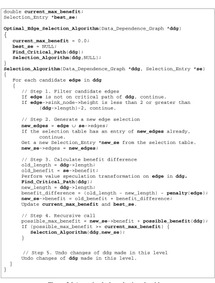
Figure 3.9 An optimal edge selection algorithm. ...51

Figure 3.10 A selection table. Each selection entry records a set of edges and its corresponding benefit. ...52

Figure 3.11 A call graph of the Selection_Algorithm for one data dependence graph in 129.compress. In each node, the first number is the called order, and the second number is the corresponding benefit that the Selection_Algorithm finds...54

Figure 3.12 The empirical running time analysis of the optimal edge selection algorithm. For all data points, the average-case complexity is y = 0.0016x3 - 0.67x2 + 67.349x - 306.35. The worst-case complexity is y = 0.1012x4 - 5.1062x3 + 80.286x2 - 416.35x + 467.08. ...56

Figure 3.13 Value prediction accuracies and BNE branch prediction accuracies of integer-register-writing operations in the SPECint95 benchmarks. ...58

Figure 3.14 BNE branch prediction accuracies sorted by their corresponding value prediction accuracies. ...58

Figure 3.15 The number of improved paths using branch misprediction penalties of 2, 5, and 10 cycles. (Note that 099.go has no improved paths in all cases.) ...61

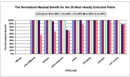
Figure 3.16 The speedup of value speculation on the 20 most heavily executed paths using branch misprediction penalties of 2, 5, and 10 cycles. (Note that 099.go has no speedups in all cases.)...62

Figure 3.17 The value prediction accuracy distribution of the selected edges (using a 10-cycle branch misprediction penalty). ...63

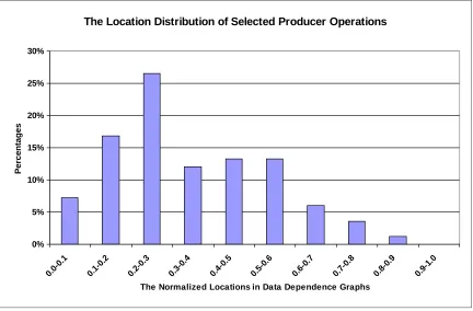
Figure 3.18 The location distribution of the selected edges (using a 10-cycle branch misprediction penalty). ...64

Figure 3.19 The location distribution of the selected producer operations in data dependence graphs (using a 10-cycle branch misprediction penalty). ...66

Figure 3.20 The location distribution of the selected consumer operations in data dependence graphs (using a 10-cycle branch misprediction penalty). ...66

Figure 4.1 An instruction format that can choose a prediction method and specify dependences for value speculation. ...71

(10)

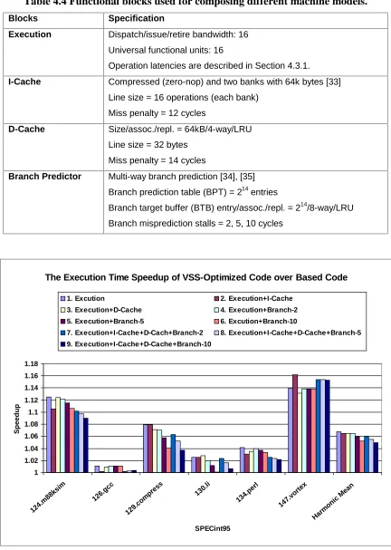
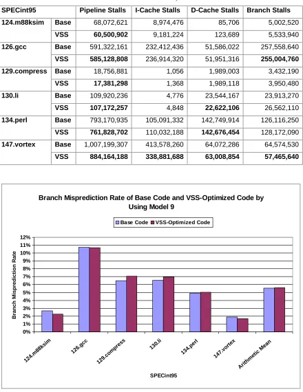
Figure 4.3 The normalized maximal benefit using the original algorithm and the algorithms with five value prediction accuracy thresholds for the 20 most heavily executed paths in SPEint95. (Note that 099.go has no benefits in all cases.)...73 Figure 4.4 The execution time speedup of VSS-optimized code over based code using nine machine models. ...79 Figure 4.5 Branch misprediction rates of base code and VSS-optimized code by using

Model 9. ...82 Figure 5.1 Examples of ILP transformation via VSS and SVSS...88 Figure 5.2 (a) The data dependence graph for code in Figure 5.1(a). (b) The data

dependence graph for code in Figures 5.1(b) or 5.1(c). Thick edges and thick-circled nodes are deleted or created by VSS or SVSS...88 Figure 5.3 Value prediction accuracies of integer-register-writing operations in the top 20 treegions in SPECint95 using hardware stride and hardware stride two-delta value predictors. ...92 Figure 5.4 The distribution of distinct stride values for predictable operations in the top 20 treegions in SPECint95...92 Figure 5.5 Value prediction accuracies using hardware stride, hardware stride two-delta, software static stride (global), and software static stride (local) value predictors for predictable operations in the top 20 treegions in SPECint95. ...95 Figure 5.6 The speedup on the 20 most heavily executed paths in each SPECint95

benchmark using hardware stride, hardware stride two-delta, and software static stride value predictors. (Note that 099.go has no speedups in all cases.)...97 Figure 5.7 The execution time speedup of SVSS-optimized code using software static stride value predictors over base code. (Note that the speedups of 126.gcc are slightly less than 1.00 on Models 2 and 3.) ...100 Figure 6.1 Profile shift between train and test input sets for all integer operations. ...108 Figure 6.2 Profile shift between train and test input sets for predictable integer operations whose prediction accuracies are higher than 90%. ...108 Figure 6.3 Profile shift between train and ref input sets for all integer operations. ...109 Figure 6.4 Profile shift between train and ref input sets for predictable integer operations whose prediction accuracies are higher than 90%. ...109 Figure 6.5 A scheme of hardware-based value profiling...111 Figure 6.6 Statistics of static operations selected by hardware-based value profiling. ...116 Figure 6.7 Statistics of dynamic operations selected by hardware-based value profiling.

(11)

(12)

List of Tables

Table 2.1 Statistics of total profiled, static and dynamic load operations. ...23

Table 3.1 Penalties under different recovery techniques for value speculation. ...35

Table 3.2 The top five opcodes and percentages of the selected producer and consumer operations (using a 10-cycle branch misprediction penalty). ...65

Table 4.1 Results of the optimal edge selection algorithm with the value prediction accuracy threshold of 90% on the 20 most heavily executed paths in SPECint95....75

Table 4.2 The code size of base code and VSS-optimized code in SPECint95. (The unit is the number of single operations.)...76

Table 4.3 The register usage in the procedures that are different between base code and VSS-optimized code. ...77

Table 4.4 Functional blocks used for composing different machine models. ...79

Table 4.5 The execution time breakdown of base code and VSS-optimized code by using Model 9. (Bold fonts indicate that VSS-optimized code performs better than base code does.) ...82

Table 4.6 Statistics of multi-way branches in base code and VSS-optimized code. Each data represents the number of multi-ops that contains a certain number of single branches from 1 to 16. ...83

Table 5.1 The top five stride values for predictable operations in SPECint95. In each grid, the first number is a stride value and the second number in parentheses is its corresponding percentage. ...93

Table 5.2 The number of global registers required for implementing software static stride value predictors on the 20 most heavily executed paths in SPECint95...98

Table 5.3 Three 16-issue VLIW machine models. ...98

Table 6.1 The train input set for the SPECint95 benchmarks. ...105

Table 6.2 The test input set for the SPECint95 benchmarks. ...105

Table 6.3 The ref input set for the SPECint95 benchmarks. ...106

Table 6.4 Statistics of total static and dynamic operations in the SPECint95 benchmarks using train, test and ref input sets. ...106

(13)

(14)

Chapter 1 Introduction

1.1 Introduction

Modern microprocessors utilize several techniques for extracting instruction-level parallelism (ILP) to improve the performance. Current techniques include register renaming to eliminate register anti- and output (false) dependences, branch prediction to overcome control dependences, and data disambiguation to resolve memory dependences [1], [41]. Recent research focuses on using value prediction [2], [3], [4] to break register flow (true) dependences, so that dependent operations can be speculatively executed without waiting for producer operations to finish. In this thesis, the technique for allowing speculative execution based on value prediction [6] is called value speculation [22].

(15)

During the fetch and dispatch stages, the value predictor generates a prediction that is forwarded to a dependent instruction prior to its execution stage. The value speculative dependent instruction must remain in a reservation station (even while its own execution continues), and be prevented from retiring. At the state-update stage, the predicted value is compared with the actual result. If the prediction is correct, the dependent instruction can then release the reservation station, update system states, and retire. If the predicted value is incorrect, the dependent instruction needs to be re-executed with the correct operand. Figure 1 illustrates the pipeline stages for value speculation utilizing a hardware-only scheme.

Figure 1.1 Pipeline stages of the hardware-only value speculation mechanism for flow dependent instructions. The dependent instruction is speculatively executed at

the same cycle as its producer instruction.

The hardware-only value speculation schemes shown in Figure 1.1 are suitable for dynamically-scheduled machines, such as superscalars, but they cannot be applied to

Fetch Dispatch Execute State- Update

Value Predictor Prediction Verification

Fetch Dispatch Execute State- Update Predicted Value

Actual Value (Predicted

Instruction) PC

(16)

statically-scheduled machines, including VLIW [20] and EPIC [27], [28] architectures. In a related approach to a different problem, the memory conflict buffer [1] was presented to dynamically disambiguate memory dependences. This allows the compiler to speculatively schedule memory references above other, possibly dependent, memory instructions. Recovery code, generated by the compiler, ensures correct program execution even when the memory dependences actually occur. Aggressively scheduling memory references that are highly likely to be independent of each other improves performance. Likewise, value-speculative scheduling attempts to improve performance by aggressively scheduling flow dependences that are highly likely to be eliminated through value prediction. Recovery code can also be used when values are mispredicted.

This thesis applies the memory conflict buffer scheme to value speculation and proposes a new combined hardware and compiler synergy, which is called value

speculation scheduling (VSS). Two new predicting and updating operations, LDPRED

(17)

• Static scheduling provides a larger scheduling scope for exploiting ILP

transformations, identifying long dependence chains suitable for value prediction, and then re-ordering code aggressively.

• Value-speculative dependent operations can be executed as early as possible before

the predicted operations that they depend on.

• The compiler controls the number of predicted values and assigns different indices to

them for accessing the value prediction table. Only operations that the compiler deems are good candidates for predictions are then predicted, reducing conflicts for the hardware.

• Recovery code is automatically generated, reducing the need for elaborate hardware

recovery techniques.

• Instead of relying on statically predicted values (e.g., from profile data), LDPRED

and UDPRED operations access dynamic prediction hardware for enhanced prediction accuracy.

• VSS can be applied to dynamically-scheduled (superscalar) processors,

statically-scheduled (VLIW) processors, or explicitly parallel instruction computing (EPIC) processors [27], [28].

• The non-intrusive design for the VSS scheme makes it easy to employ value

prediction and value speculation in future microprocessors.

(18)

algorithm is designed to solve the optimal edge selection problem efficiently. Running the optimal edge selection algorithm finds an optimal set of edges (dependences) and the corresponding maximal benefit from value speculation. Examining the selected dependences provides insights into the instruction selection techniques that relate to the success of utilizing value speculation to improve the performance of microprocessors. Also, the optimal edge selection algorithm serves as a new compilation phase of benefit analysis to expose selected dependences to dynamically-scheduled and statically-scheduled machines. The compiler-directed edge selection can alleviate the burden for the hardware to decide which dependences should be broken at run-time.

Software-only value speculation scheduling (SVSS) is proposed and can be

applied to existing microprocessors for improving the performance. The SVSS scheme utilizes software static stride value predictors to generate value predictions, so that dependent operations can be value-speculatively executed. The experimental results show that the performance of the software static stride value predictor is comparable to that of the hardware stride two-delta value predictor [10], [13]. Significant speedups are shown for applying SVSS to the SPECint95 benchmarks.

(19)

results, the proposed scheme of hardware-based value profiling can accurately identify highly predictable operations at run-time. The VSS optimization is experimented based on the feedback from hardware-based value profiling.

1.2 Research Contributions

The research contributions of this thesis are as follows.

• This thesis proposes value speculation scheduling (VSS) to exploit the value

predictability of operations to improve the performance of microprocessors. The VSS technique leverages advantages of both hardware schemes for value prediction and compiler schemes for exposing ILP.

• Two new predicting and updating operations, LDPRED and UDPRED, are proposed

to be the interface between the value predictor and program code.

• A value speculation scheduling algorithm is proposed to utilize LDPRED and

UDPRED operations to break critical paths in a program to shorten execution time.

• A value speculation model is built as solving an optimal edge selection problem in a

data dependence graph to understand and improve the techniques for value speculation.

• Three properties are observed from the optimal edge selection problem and help to

design an efficient optimal edge selection algorithm.

• Running the optimal edge selection algorithm serves as a new compilation phase of

(20)

value prediction. The selected dependences are then exposed to the hardware or the compiler to obtain maximal benefits from value speculation.

• Software-only value speculation scheduling (SVSS) is proposed and can be applied to

existing microprocessors for improving the performance.

• Software static stride value predictors are designed to have comparable performance

to hardware stride two-delta value predictors.

• Hardware-based value profiling is proposed to accurately collect highly predictable

operations at run-time with fewer overheads.

1.3 Outline of the Thesis

(21)

Chapter 2 Value Speculation Scheduling

(22)

The remainder of this chapter is organized as follows. Section 2.1 presents the microarchitectural support for value speculation scheduling (VSS). Section 2.2 examines the value predictor design for VSS. Section 2.3 introduces the VSS algorithm. Section 2.4 presents experimental results and discusses the heuristics used in the VSS scheme. Section 2.5 concludes this chapter.

2.1 Microarchitectural Support for VSS

Hardware pipeline stages for the VSS scheme are shown in Figure 2.1. Two new predicting and updating operations, LDPRED and UDPRED, are introduced to be the interface with the value predictor during the execution stage. An LDPRED operation loads a predicted value generated by the value predictor into a specified general-purpose register. A UDPRED operation updates the value predictor with the actual result, resetting the device for future predictions after a misprediction. In Figure 2.1 of the VSS scheme, the microprocessor only needs to add a new value predictor and slightly modify the pipeline for accessing the value predictor at the execution stage. The non-intrusive design makes it easy to incorporate the VSS scheme into future microprocessors.

(23)

Figure 2.1 Pipeline stages of the VSS scheme. Two new operations, LDPRED and UDPRED, are introduced to be the interface with the value predictor during the

execution stage.

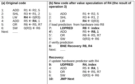
(a) Original code

1: ADD R1 Ä R2, 5 2: SHL R3 Ä R1, 2 3: LW R4 Ä 0(R3) 4: ADD R5 ÄR4, 1 5: OR R6 Ä R5, R7 6: SW 0(R3) Ä R6 Next: ...

(b) New code after value speculation of R4 (the result of operation 3)

1: ADD R1 Ä R2, 5 2: SHL R3 Ä R1, 2 3: LW R4 Ä 0(R3) // load prediction from hardware into R8 7: LDPRED R8 Ä index 4’: ADD R5 Ä R8, 1 5’: OR R6 Ä R5, R7 6’: SW 0(R3) Ä R6 // verify prediction

8: BNE Recovery R8, R4 Next: ...

Recovery:

// update hardware predictor with R4 9: UDPRED R4, index 4: ADD R5 ÄR4, 1 5: OR R6 Ä R5, R7 6: SW 0(R3) Ä R6 10: JMP Next

Figure 2.2 An example of value speculation scheduling.

Fetch Dispatch Execute State- Update

Value Predictor

Predicted Value LDPRED

(24)

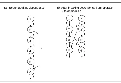
Figure 2.3 shows the data dependence graphs for the code sequence of Figure 2.2 before and after breaking the flow dependence from operation 3 to operation 4. Assume that the latencies of arithmetic, logical, branch, store, LDPRED, and UDPRED operations are 1 cycle, and that the latency of load operations is 2 cycles. Then, the schedule length of the original code sequence of Figure 2.3(a), operations 1 to 6, is seven cycles. By breaking the flow dependence from operation 3 to operation 4, VSS results in a schedule length of five cycles. Figure 2.3(b) illustrates the schedule now possible due to reduced overall dependence height and ILP exposed in the new data dependence graph. This improved schedule length, from seven cycles to five cycles, does not consider the penalty associated with value misprediction due to the required execution of recovery code. The impact of recovery code on performance will be discussed in Section 2.3.

(25)

UDPRED operation and the original dependent operations 4, 5, and 6. After executing recovery code, the program jumps to the next operation after operation 8 and execution proceeds as normal. Note that in Figure 2.2(b) operations 4’, 5’, and 6’ use speculative versions [41] of original operations 4, 5, and 6. If the store, operation 6, does not have the speculative version, the compiler must not destroy data values belonging to other memory locations, i.e. the memory address of the store must be non-speculative. As shown in Figure 2.2(b), for aggressive optimization, the compiler may allow the store, operation 6’, to save wrong data values to the memory location of 0(R3), which is non-speculative.

Figure 2.3 Data dependence graphs for code in Figure 2.2. The numbers along each edge represent the latency of each operation. In (a), the schedule length is seven

cycles. In (b), because of exposed ILP and dependence height reduction, the schedule length is reduced to five cycles.

1

2

3 1

1

2

8 1 1

2

3 1

1

2

4

5 1

1

6 1

7

4’

5’ 1

1

6’ 1 1

1

(26)

Each LDPRED and UDPRED pair that corresponds to the same value prediction uses the same table entry index into the value predictor. Each index is assigned by the compiler to avoid unnecessary conflicts inside the value predictor. While the number of table entries is limited, possible conflicts are deterministic and can be factored into choosing which values to predict in a compiler approach. A value predictor design, featuring the new LDPRED and UDPRED operations, will be described in Section 2.2.

By combining hardware and compiler techniques, the strengths of both dynamic and static techniques for exploiting ILP can be leveraged. We see several possible advantages to VSS:

• Static scheduling provides a larger scheduling scope for exploiting ILP

transformations, identifying long dependence chains suitable for value prediction, and then re-ordering code aggressively.

• Value-speculative dependent operations can be executed as early as possible before

the predicted operations that they depend on.

• The compiler controls the number of predicted values and assigns different indices to

them for accessing the prediction table. Only operations that the compiler deems are good candidates for predictions are then predicted, reducing conflicts for the hardware.

• Recovery code is automatically generated, reducing the need for elaborate hardware

recovery techniques.

• Instead of relying on statically predicted values (e.g., from profile data), LDPRED

(27)

• VSS can be applied to dynamically-scheduled (superscalar) processors,

statically-scheduled (VLIW) processors, or explicitly parallel instruction computing (EPIC) processors [27], [28].

• The non-intrusive design for the VSS scheme makes it easy to employ value

prediction and value speculation in future microprocessors.

There is a drawback to the VSS scheme. Because static scheduling techniques are employed, value-speculative operations are committed to be speculative and therefore always require predicted values. Hardware-only schemes can dynamically decide when it is appropriate to speculatively execute operations. The dynamic decision is based on the value predictor’s confidence in the predicted value, avoiding misprediction penalties for low confidence predictions.

2.2 Value Predictor Design

(28)

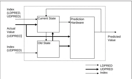
Figure 2.4 shows the block diagram of a value predictor that includes LDPRED and UDPRED operations. In this value predictor, there are three fundamental units, the

current state block, the old state block, and the prediction hardware block. The current state block may contain register values, finite state machines, history information, or

machine flags, depending on the prediction method employed. The old state block hardware is a duplicate of the current state block hardware. The prediction hardware block generates predictions with the input from the current state block. Various prediction mechanisms can be used. For example, generating the prediction as the last value (last value predictors [2], [3]). Or, generating the prediction as the sum of the last value and the stride, which is the difference between the most recent last values (stride predictors [4], [6], [10], [13]). Also, two-level value predictors [13] and context-based value predictors [10], [11] allow for the prediction of recently computed values. For two-level predictors, a value history pattern indexes a pattern history table, which in turn is used to index a value prediction from recently computed values. Two-level value prediction hardware is based on two-level branch prediction hardware.

(29)

hardware is updated simultaneously with the current state block update. Note that for the LDPRED operation, the predicted value is used to update the current state speculatively.

Figure 2.4 The block diagram of value predictor design featuring LDPRED and UDPRED operations.

The compiler assigned number also indexes the operation of the UDPRED operation. When the value prediction is incorrect, the recovery code in Figure 2.2(b) must be executed. The execution of UDPRED operations only occurs in recovery code, or only when values are mispredicted. The UDPRED operation causes the update of both the current state block and the prediction hardware with the actual computed value and the old state block.

If the compiler can ensure that each LDPRED and UDPRED pair is executed in turn (each prediction is verified and value predictions are not nested), the old state block

Current State

Old State

Prediction Hardware

Actual Value (UDPRED) Index (LDPRED, UDPRED)

Index (UDPRED)

Predicted Value

(30)

requires only one table entry. The same table entry in the old state block is updated by every LDPRED operation, and used by every UDPRED operation, in the case of misprediction.

(31)

Figure 2.5 The hybrid predictor (with stride and two-level predictors). Saturating counters are compared to select between the prediction techniques.

2.3 A Value Speculation Scheduling Algorithm

Performance improvement for value speculation scheduling (VSS) is affected by prediction accuracy, the number of saved cycles (from schedule length reduction), and the number of penalty cycles (from execution of recovery code). Suppose that after breaking a flow dependence, value-speculative dependent operations are speculated, saving S cycles in overall schedule length when the prediction is correct. Recovery code is also generated and requires P cycles. Prediction accuracy for the speculated value is X. In this case, speedup may be positive if S > (1-X) * P holds. For the example of Figure 2.3(b), VSS saves 2 cycles (from 7 cycles to 5 cycles) and the resulting recovery code contains 5 operations, requiring 3 cycles in an ILP processor. Therefore, for positive speedup, the prediction accuracy must be at least 33%. If the actual prediction accuracy

Prediction Index Stride

Predictor

2:1 MUX

Two-Level Predictor

Counter for Stride Predictor

CMP ( > )

(32)

is less, performance will be degraded by VSS. In Section 3.1, the penalties for value misprediction in the VSS scheme will be discussed in more detail. With these performance considerations in mind, an algorithm for VSS is proposed in Figure 2.6.

The first step is to perform value profiling. The scheduler must select highly predictable operations to improve performance through VSS. Results from value profiling under different inputs and parameters have been shown to be strongly correlated [4], [7]. Therefore, value profiling can be used to select highly predictable operations on which to perform value speculation.

Value profiling can be performed for all register-writing operations. If profiling overhead is a concern, a filter may be used to perform value profiling only on select operations. Select operations may be those that reside on critical paths (long dependence heights) or those that have long latencies (e.g., load operations). In [7], estimating and convergent profiling are proposed to reduce profiling overhead for determining the invariance of operations. Similar techniques could be applied for determining the value predictability of operations.

Next, the value speculation scheduler performs region formation. Treegion formation [17] is the region type chosen for our experiments. A treegion is a non-linear region that includes multiple execution paths in the form of a tree of basic blocks. The larger scheduling scope of treegions allows the scheduler to perform aggressive control speculation [41] and value speculation. A data dependence graph is then constructed for each region.

(33)

queries the value profiling information to get the estimate of its predictability. If the predictability estimate is greater than the threshold, value prediction is performed. For aggressive scheduling, more operations can be speculated by choosing a low threshold. Suggested values for the threshold are derived from experimental results in Section 2.4.

1. Perform value profiling 2. Perform region formation

3. Build a data dependence graph for a region

4. Select an operation with its prediction accuracy (based on value profiling) greater than a threshold

5. Insert LDPRED after the predicted operation (the selected operation of step 4)

6. Change the source operand of the dependent operation(s) to the destination register of LDPRED

7. Insert a branch to recovery code

8. Generate recovery code (which contains UDPRED) 9. Repeat steps 4 – 8 until no more candidates found 10. Update the data dependence graph for a region 11. Perform instruction scheduling for a region 12. Repeat steps 2 – 11 for each region

Figure 2.6 A value speculation scheduling algorithm.

(34)

one chain of dependent operations may result from just one value prediction, only one LDPRED operation is needed for each value prediction.

In step seven, a branch to recovery code is inserted for repairing value misprediction. Only one branch per data value prediction is required and the scheduler determines where this branch is inserted. Once the location of the branch is set, all operations in all dependence chains between the predicted operation and the branch to recovery code are candidates for value-speculative execution. It is therefore desirable to schedule any of these operations above the predicted operation. Actual hardware resources will restrict the ability to speculatively execute these candidates for value speculation. Also, as all candidates for value speculation are duplicated in recovery code, their number directly affects the penalty for value misprediction. These factors affect the scheduler’s decision on where to place the branch to recovery code. Moreover, the compiler needs to make sure that all source operands (e.g., register values and memory data values) of candidate operations between the predicted operation and the branch are protected, so that inside recovery code value-speculative operations can be re-executed with original operands in the case of value misprediction.

(35)

of the predicted operation (the actual result of the predicted operation). The UDPRED operation index and the actual result are used to update the value predictor.

Finally, in steps ten and eleven, the data dependence graph is updated to reflect the changes and instruction scheduling for the region is performed. Because of the machine resource restrictions and dependences, not all candidates for value speculation are speculated above the predicted operation. Section 2.4 shows the results of using different threshold values for determining when to do value speculation.

2.4 Experimental Results

The SPECint95 benchmark suite was used in the experiments. All programs were compiled with classic optimizations by the IMPACT compiler from the University of Illinois [18] and converted to the Rebel textual intermediate representation by the Elcor compiler from Hewlett-Packard Laboratories [19]. Then, the LEGO compiler, a research compiler developed at North Carolina State University, was used to insert profiling code, form treegions, and schedule operations [17]. After instrumentation for value profiling, intermediate code from the LEGO compiler was converted to C code. Executing the resultant C code generated profiling data.

(36)

load operations represents the number of load operations that are actually executed. The difference between total profiled and static load operations is the number of load operations that are not visited. The number of dynamic load operations is the total of each load operation executed multiplied by its execution frequency.

Table 2.1 Statistics of total profiled, static and dynamic load operations.

SPECint95 Total Profiled Load Operations

Static Load Operations

Dynamic Load Operations

099.go 7,702 6,370 86,613,967

124.m88ksim 2,954 747 15,765,232

126.gcc 35,948 17,418 132,178,579

129.compress 96 72 4,070,431

130.li 1,202 414 24,325,835

132.ijpeg 5,104 1,543 118,560,271

134.perl 6,029 1,429 4,177,141

147.vortex 16,587 10,395 527,037,054

Stride, two-level, and hybrid value predictors were simulated during value profiling to evaluate prediction accuracy for each load operation. During value profiling, after every execution of a load operation, the simulated prediction is compared with the actual value to determine prediction accuracy. The value predictor simulators are updated with actual values, as they would be in hardware, to prepare for the prediction of the next use. Since the goal of value profiling is to measure the potential prediction accuracy of operations rather than the required capacities of the hardware buffers, no index conflicts between operations are modeled.

(37)

stride equals the difference between the most recent current values. The stride value predictor always generates a prediction. No finite state machine hardware is required to determine if a prediction should be used.

The two-level value predictor design is as in [13], with four data values and six outcome value history patterns in the value history table of the first level. The value history patterns index the pattern history table of the second level. The pattern history table employs four saturating counters, used to select the most likely prediction amongst the four data values. The saturating counters in the pattern history table increase by three, up to twelve, and decrease by one, down to zero. Selecting the data value with the maximum saturating counter value always generates a prediction.

The hybrid value predictor of stride and two-level value predictors utilizes the previous description illustrated earlier in Figure 2.5. In the hybrid design, the saturating counters, used to select between stride and two-level prediction, also increase by three, up to twelve, and decrease by one, down to zero.

(38)

Prediction Accuracy of Load Operations Using Stride, Two-level, and Hybrid Value Predictors 0% 10% 20% 30% 40% 50% 60% 70% 80% 90% 100% 099. go 124. m88 ksim 126. gcc 129. com pres s 130. li 132. ijpeg 134. perl 147. vor tex Ari thm etic Mea n SPECint95 Accu racy

Stride Two-Level Hybrid

Figure 2.7 Prediction accuracies of load operations using stride, two-level, and hybrid predictors.

(39)

The VSS algorithm shown in Figure 2.6 was performed on all SPECint95 programs. Prediction accuracy threshold values of 90%, 80%, 70%, 60% and 50% were evaluated. The number of candidates for value-speculative execution was limited to three for each value prediction. This parameter was varied in our evaluation, with the value of three providing good results.

(40)

Figure 2.8 The prediction accuracy distribution for static load operations using the hybrid predictor.

Figure 2.9 The prediction accuracy distribution for dynamic load operations using the hybrid predictor.

Hybrid Predictor 0 10 20 30 40 50 60 70 80 90 100

≥90% ≥80% ≥70% ≥60% ≥50% ≥40% ≥30% ≥20% ≥10% ≥0%

Prediction Accuracies

Percentage of Dynam

ic Load (%

) 099.go 124.m88ksim 126.gcc 129.compress 130.li 132.ijpeg 134.perl 147.vortex Hybrid Predictor 0 10 20 30 40 50 60 70 80 90 100

≥90% ≥80% ≥70% ≥60% ≥50% ≥40% ≥30% ≥20% ≥10% ≥0%

(41)

Figure 2.10 shows the execution time speedup of programs scheduled with VSS over without VSS. Five different prediction accuracy thresholds were used to select which load operations are value speculated. The maximum speedup for all benchmarks is 17% for 147.vortex. As illustrated in Figure 2.9, 147.vortex has many dynamic load operations that are highly predictable. While 147.vortex does not have the highest predictability for load operations, the sheer number, as illustrated in Table 2.1, results in the best performance. Benchmarks 124.m88ksim and 129.compress also show impressive speedups, 10% and 11.5% respectively, using a threshold of 50%. Speedup for 124.m88ksim actually goes up, even as the prediction accuracy threshold goes down, from 90% to 50%. This result can be deduced from the distribution of dynamic loads. For 124.m88ksim, there is a steady increase in the number of dynamic loads available as the threshold decreases from 90% to 50%. There is a tapering off in speedup though, as more mispredictions are seen near a threshold of 50%. For 129.compress, the step in the distribution of dynamic loads from 80% to 70% is reflected in a corresponding step in speedup. Performance gains for 126.gcc are more reflective of the large number of dynamic load operations than of their predictability. Penalties for misprediction at the lower thresholds reduce speedup for 126.gcc. Benchmark 130.li, with a distribution of dynamic loads similar to 126.gcc, has lower performance due to fewer dynamic loads. Benchmark 134.perl clearly suffers from not having many dynamic loads. Benchmarks 099.go and 132.ijpeg do not have good predictability for load operations.

(42)

Choosing a threshold of predictability lower than 70% results in a tapering off in performance for some benchmarks. This is due to both higher penalties for value misprediction and saturation of functional unit resources, resulting in fewer saved execution cycles.

The Execution Time Speedup on 8U Machine Model

1 1.02 1.04 1.06 1.08 1.1 1.12 1.14 1.16 1.18 099 .go 124 .m88 ksim 126 .gcc 129 .comp

ress ₁₃₀.li 132 .ijpeg 134 .per l 147 .vor tex SPECint95 S p e e dup

90% 80% 70% 60% 50%

Figure 2.10 The execution time speedup for programs scheduled with VSS over without VSS. Prediction accuracy threshold values of 90%, 80%, 70%, 60% and

50% are used.

2.5 Summary

(43)

(44)

Chapter 3 Modeling Value Speculation

(45)

critical paths. However, it is unknown whether these heuristics do a good job of obtaining maximal benefits from value speculation.

To understand and improve the techniques for value speculation, we model value speculation as an optimal edge selection problem. Edges represent dependences between operations in a data dependence graph. The optimal edge selection problem involves finding an optimal (minimal) set of edges to break that achieves maximal benefits from value speculation, while taking the penalties for value misprediction into account. Based on three properties observed from the optimal edge selection problem, an efficient algorithm is designed using the techniques of branch-and-bound and memoization (a variation of dynamic programming) [21]. After running the optimal edge selection algorithm, several experimental results of modeling value speculation are presented in this chapter, including:

• The maximal benefits from value speculation on the 20 most heavily executed paths

in the SPECint95 benchmarks.

• The impact of different penalties for branch misprediction on the benefits.

• The value prediction accuracy distribution and the location distribution of an optimal

set of edges (dependences).

• The location distribution of the selected producer and consumer operations.

• The top five opcodes of the selected producer and consumer operations.

(46)

algorithm, with experimental results shown in Section 3.5. Section 3.6 concludes this chapter.

3.1 Introduction of Value Speculation

The techniques for value speculation in dynamically-scheduled and statically-scheduled machines are introduced as follows. In dynamically-statically-scheduled machines [2], [3], there is an instruction window that maintains a pool of instructions waiting to be executed. All instructions in the instruction window dynamically form a data dependence graph. Without the value prediction technique, the dynamic scheduler selects an instruction to execute only if all of its operands are ready. However, by using value prediction to break flow dependences, the original data dependence graph can be collapsed and instructions can be speculatively executed even if their operands are not ready. Speculatively executed instructions must wait for verifying predicted values before their retirement. In the case of value misprediction, recovery mechanisms are required to re-execute instructions with correct operands. One recovery scheme utilizes the branch misprediction handling hardware [8] that is already in the dynamically-scheduled machine. All instructions following the incorrectly predicted instruction are re-fetched and re-executed. Another recovery mechanism is the selective re-issuing scheme [2], [3] to re-execute dependent instructions that are affected by incorrect predictions. The implementation of the selective re-issuing scheme is more complicated than that of the branch misprediction handling hardware.

(47)

region. The scheduler must honor all dependences among operations to generate a correct schedule. With the help of value prediction and value speculation, the scheduler can break true dependences and speculatively schedule value-dependent operations. The compiler inserts predicting operations, LDPRED [22], to load a prediction from the value predictor, and verifying operations, BNE (branch if not equal) [22], to compare the predicted value with the actual result. In the case of value misprediction, the compiler can provide recovery code [22] for re-executing operations, or advanced hardware can generate recovery code on the fly and execute recovery code on a separate compensation engine [25].

(48)

Table 3.1 Penalties under different recovery techniques for value speculation.

Dynamically-Scheduled Machines Statically-Scheduled Machines Recovery

Techniques Branch Misprediction Handling Hardware [8]

Selective Re-issuing [2], [3]

Compiler-Generated Recovery Code [22] Hardware-Generated Recovery Code [25] Penalties for Verifying Value Prediction

1 cycle (for comparing actual and predicted values) always + Flushing all pipeline stages when value is mispredicted

1 cycle (for comparing actual and predicted values) always

1 cycle (for comparing actual and predicted values) always + Flushing all pipeline stages when the BNE operation is mispredicted

1 cycle (for comparing actual and predicted values) always Penalties for Re-execution Re-executing all operations when value is mispredicted Re-executing only affected operations when value is mispredicted Re-executing only affected operations when value is mispredicted Re-executing only affected operations when value is mispredicted (on a separate engine) I-Cache Stalls Re-fetching all

operations when value is

mispredicted +

Side effect of speculative execution

Fetching recovery code when value is mispredicted +

Side effect of speculative execution D-Cache Stalls, Structure Hazards

(49)

As shown in Table 3.1, the scheme of compiler-generated recovery code for statically-scheduled machines has the penalties of one cycle for verifying the predicted value, the flushing cycles after the verifying operation (BNE) is mispredicted, the cycles for executing recovery code, additional I-Cache stalls for fetching recovery code, and extra stalls due to the impact of speculative execution on the I-Cache, D-Cache, and machine resources. In Table 3.1, some items of penalties are the same under different recovery mechanisms, but others are different.

3.2 An Optimal Edge Selection Problem

3.2.1 Terminology of Data Dependence Graphs

In related work [14], a dynamic data dependence graph is utilized to study the available parallelism with data value prediction. For modeling value speculation, the data dependence graph is heavily used as well. Terminology required on the data dependence graph is introduced as follows.

The data dependence graph that is formed in the instruction window or generated by an acyclic code scheduler is a directed acyclic graph (DAG). The data dependence graph is denoted by DDG=(N, E), where N is the set of Nodes representing operations and E is the set of Edges representing dependences between operations. For an edge Ei,

Source(Ei) is the source node of the edge Ei and Sink(Ei) is the sink node of the edge Ei.

(50)

Register flow and output dependences have latencies equal to the latencies of source operations. Register anti-, memory, and control dependences have latencies of zeros.

Each node has a Height, which is the latest scheduled cycle without delaying other operations. A top-down depth-first-search (DFS) algorithm [21] shown in Figure 3.1 can compute heights of all nodes in a data dependence graph. The running time of computing heights is O(|N| + |E|), where |N| is the number of nodes and |E| is the number of edges. The node also has a Depth, which is the earliest scheduled cycle of the operation. Depths are calculated by a bottom-up DFS algorithm, very similar to the algorithm shown in Figure 3.1. Only heights are used in this chapter. The maximal height of all nodes in the DDG represents the minimal cycles to execute or schedule all operations in the DDG. It is denoted by |DDG|, and called the Length or the Height of the DDG.

(51)

// Compute heights of all nodes in a DDG

Compute_Height(DDG) {

// Step 1. Reset height of nodes and length of DDG. DDG->length = -1;

For each node in DDG { node->height = -1; }

// Step 2. Compute height for each node in DDG {

height = Compute_Height(node); if(height > DDG->length) { DDG->length = height; }

}

// Step 3. Reverse heights of all nodes, so heights are the // latest scheduled cycle.

for each node in DDG {

node->height = DDG->length – node->height; }

}

// Compute height of this node int Compute_Height(node)

{

// Step 1. If node has height, return its height. If (node->height != -1) {

return node->height; }

// Step 2. Get the max height from its successors. max_height = 0;

for each succ_edge of node { sink_node = succ_edge->sink;

succ_height = Compute_Height(sink_node);

new_height = succ_height + succ_edge->latency; if(new_height > max_height) {

max_height = new_height; )

}

if node has no succ_edge

node->height = node->op->latency; else

node->height = max_height;

return node->height; }

(52)

// Find all critical paths in a DDG

Find_Critical_Path(DDG) {

// Step 1. Compute heights of nodes in the DDG. Compute_Height(DDG);

// Step 2. Reset critical attributes of nodes and edges. for each node in DDG {

node->critical = false;

for each succ_edge of node { succ_edge->critical = false; }

}

// Step 3. Find critical paths from nodes with height 0. for each node in DDG {

if (node->height == 0) { node->critical = true; Find_Critical_Path(node); }

} }

// Find critical path starting from node

Find_Critical_Path(node) {

for each succ_edge of node { sink_node = succ_edge->sink;

if (sink_node->height == (node->height + succ_edge->latency)) { succ_edge->critical = true;

if(sink_node->critical == false) { sink_node->critical = true;

Find_Critical_Path(sink_node); }

} } }

(53)

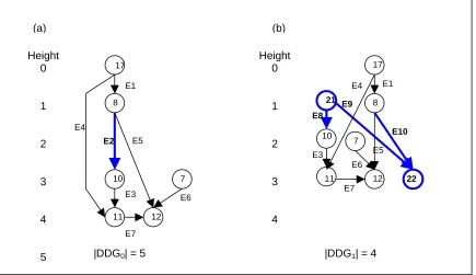
Figure 3.3 (a) A data dependence graph. (b) A modified data dependence graph after performing the value speculation transformation on E2 (from node 8 to node

10). Thick edges and thick-circled nodes are on the critical path.

3.2.2 The Problem Statement

The model of value speculation is best illustrated by an example. For the data dependence graph shown in Figure 3.3(a), one edge E2, from node 8 to node 10, is

selected by the value speculation technique. In Figure 3.3(b), the value speculation

transformation is performed, including breaking the edge E2 (from node 8 to node 10),

adding one predicting node 21 (LDPRED), adding one verifying node 22 (BNE), adding one edge E8 (from node 21 to node 10), adding one edge E9 (from node 21 to node 22),

and adding one edge E10 (from node 8 to node 22). The predicting node loads a

prediction from a value predictor, and feeds its result to node 10. The verifying node compares the predicted value from the predicting node and the actual result of node 8.

Height 0 1 2 3 4

|DDG0| = 5 |DDG1| = 4

17 8 11 12 7 10 7 21 22

(a) (b)

(54)

Note that the predicting and verifying nodes are explicit in statically-scheduled machines, but are implicit in dynamically-scheduled machines.

In Figure 3.3(a), the length of the DDG is 5 cycles. In Figure 3.3(b), after performing the value speculation transformation, the length of the modified DDG is reduced to 4 cycles. The modified DDG, denoted by DDGn, is obtained after performing

the value speculation transformation on n edges in the original DDG. The original DDG without performing the value speculation transformation on any edge is DDG0.

In the case of value misprediction, penalties are incurred for recovery. The total penalty for mispredicting node Ni is denoted by Penalty(Ni). It is assumed to be greater

than zero. Based on Penalty(Ni), the penalty for mispredicting edge Ei, Penalty(Ei), is

defined as follows:

Penalty(Ei) =    already. predicted been has E of node source the if 0, yet. predicted been not has E of node source the if )), urce(E Penalty(So i i i

Because Penalty(Ni) is counted at most once in the proposed model, if the source

node of Ei has not been predicted yet, Penalty(Ei) equals Penalty(Source(Ei)) after

performing the value speculation transformation on the edge Ei. Otherwise, Penalty(Ei) is

zero. Note that in the latter case of Penalty(Ei) equal to zero, the predicting node, the

(55)

For an acyclic data dependence graph DDG=(N, E), find a minimal set of edges as {E1,

E2, …, En-1, En}, such that the benefit is maximal (and must be greater than zero) by

performing the value speculation transformation on selected edges. The benefit for the DDG is defined as follows.

Benefit(DDG) = Benefit(DDG0)

= Execution_cycles_of_DDG0 - Execution_cycles_of_DDGn

= |DDG0| - (|DDGn| +

∑

=

n

i 1

Penalty(Ei))

= (|DDG0| - |DDGn|) -

∑

=

n

i 1

Penalty(Ei)

= Cycle_savings – Misprediction_penalties where

Penalty(Ni) > 0 for all nodes,

Penalty(Ei) =    already. predicted been has Ei of node source the if 0, yet. predicted been not has Ei of node source the if urce(Ei)), Penalty(So

Figure 3.4 An optimal edge selection problem.

Penalty(Ni) = Value_misprediction_rate * Cycles_of_recovery_code +

BNE_branch_misprediction_rate * Stall_cycles_of_mispredicted_branch where

Cycles_of_recovery_code = |DDG0| – Height (Ni),

Stall_cycles_of_mispredicted_branch = 2, 5, or 10,

Value misprediction rates and BNE branch misprediction rates come from profile results.

(56)

Using the introduced terminology, value speculation is modeled as an optimal edge selection problem that is formally presented in Figure 3.4. The optimal edge selection problem asks for finding a minimal set of edges such that the benefit is maximal (and must be greater than 0) by performing the value speculation transformation on selected edges.

Some assumptions and limitations of the proposed value speculation model are as follows:

• The data dependence graph must be a directed acyclic graph (DAG). The DDG is

constructed for operations in the instruction window of dynamically-scheduled machines, or for operations in a linear path (trace) of basic blocks in a program for statically-scheduled machines.

• The selected edge must belong to the original set of edges, and must be a flow (true)

dependence type.

• In the optimal edge selection problem, the latencies of edges and the penalties for

(57)

stalls, and structural hazards are ignored. In the equation, the value misprediction rates and the BNE branch misprediction rates come from profile results.

• Machine resources are not taken into account in the optimal edge selection problem.

Unlimited resources are assumed to be available for the value speculation techniques.

• In dynamically-scheduled machines, instructions shift into and out of the instruction

window every cycle. However, the proposed value speculation model focuses only on a static data dependence graph that is composed of the instructions in the current instruction window.

3.3 Three Properties Observed from the Optimal Edge

Selection Problem

The optimal edge selection problem presented in Figure 3.4 can be solved by a brute-force method that measures the benefits of all possible edge selections. For |E| edges, the brute force method must try 2|E| combinations. However, from observing the optimal edge selection problem, there exist some properties for us to design an efficient algorithm.

The first observation is that because the process of the value speculation transformation is deterministic, the final DDGn should be the same regardless of the order

of the value speculation transformation performed on the selected edges in the DDG0.

(58)

Property 1: Decomposition

Let Benefit_Difference(Ei) = |DDGi-1| - |DDGi| - Penalty(Ei). Then, for a set of edges

{E1, E2, …, En-1, En}, the benefit for the DDG0 is the summation of all benefit

differences.

Figure 3.6 Property 1 of the optimal edge selection problem: decomposition.

Proof of Property 1:

For the presentation, the index of the edges {E1, E2, …, En-1, En} is coincidently the same

as the order when they are selected. The benefit for the DDG0 after performing the value

speculation transformation on {E1, E2, …, En-1, En} is denoted by

Benefit(DDG0)

= (|DDG0| - |DDGn|) -

∑

=

n

i 1

Penalty(Ei)

= (|DDG0| - |DDG1|) + (|DDG1| - |DDG2|) + … + (|DDGn-1| - |DDGn|) -

∑

=

n

i 1

Penalty(Ei)

= (|DDG0| - |DDG1| - Penalty(E1)) + (|DDG1| - |DDG2| - Penalty(E2)) + … + (|DDGn-1| -

|DDGn| - Penalty(En))

=

∑

=

n

i 1

(|DDGi-1| - |DDGi| - Penalty(Ei))

=

∑

=

n

i 1

Benefit_Difference(Ei). #

(59)

transformation on {E2}, {E5} will be an optimal solution for the DDG1 shown in Figure

3.3(b). (Note that for the modified DDG, we restrict that the candidate edge must still belong to the original set of edges in the DDG0, and must be a true dependence type.)

Property 2 is shown in Figure 3.7, and its proof appears as follows.

Property 2: Optimal Substructure

For an optimal set of edges {E1, E2, …, En-1, En} for the DDG0, after performing the

value speculation transformation on a subset of optimal edges, the remaining edges in the optimal set of edges is an optimal solution for the modified DDG. So, the problem of each modified DDG is also an optimal edge selection problem.

Figure 3.7 Property 2 of the optimal edge selection problem: optimal substructure.

Proof of Property 2: (By Contradiction)

Because {E1, E2, …, En-1, En } is an optimal solution for the DDG0, {E1, E2, …, En-1, En }

should be the minimal set of edges that yield the highest positive benefit for the DDG0.

Without loss of generality, {E1, E2, …, En-1, En} is split into two sets of edges, {E1, E2,

…, Ek} and {Ek+1, …, En-1, En}. For the presentation, the index of the edges {E1, E2, …,

En} is coincidently the same as the order when they are selected. From Property 1, the

maximal benefit for the DDG0 is denoted by Benefitold(DDG0)

=

∑

=

n

i 1

=

∑

=

k

i 1

(|DDGi-1| - |DDGi| - Penalty(Ei)) +

∑

+ =

n

k i 1

(60)

Let Benefitold(DDGk) =

∑

+ =

n

k i 1

(|DDGi-1| - |DDGi| - Penalty(Ei)). Then,

Benefitold(DDG0) =

∑

=

k

i 1

(|DDGi-1| - |DDGi| - Penalty(Ei)) + Benefitold(DDGk).

Property 2 states that {Ek+1, …, En-1, En} must be an optimal solution for the DDGk. We

will prove it by the following four cases.

Case 1. If we assume that {Ek+1, …, En-1, En} does not yield the highest benefit for the

DDGk, one new Benefitnew(DDGk) can be found to be higher than the Benefitold(DDGk).

Adding

∑

=

k

i 1

(|DDGi-1| - |DDGi| - Penalty(Ei)) and the Benefitnew(DDGk) together, one

new Benefitnew(DDG0) can be found to be higher than the Benefitold(DDG0). This

contradicts that the Benefitold(DDG0) should be maximal. Therefore, we cannot find

other set of edges for the DDGk to have higher benefits than

∑

+ =

n

k i 1

(|DDGi-1| - |DDGi| -

Penalty(Ei)).

Case 2. If we assume that {Ek+1, …, En-1, En} for the DDGk is not the minimal set of

edges that yield the maximal benefit (= Benefitold(DDGk)), a smaller set of edges {Ek’+1,

…, En’-1, En’} can be found to have the same benefit (=Benefitold(DDGk)). Combining

{E1, E2, …, Ek} and {Ek’+1, …, En’-1, En’} forms a smaller set of edges for the DDG0 that

yield the benefit equal to the Benefitold(DDG0). This contradicts that {E1, E2, …, En-1,

En} should be the minimal set of edges for the DDG0. Therefore, {Ek+1, …, En-1, En} is

the minimal set of edges that yield the maximal benefit (= Benefitold(DDGk)) for the

(61)

Case 3. If we assume that

∑

+ = n k i 1

(|DDGi-1| - |DDGi| - Penalty(Ei)) is zero, performing value

speculation transformation on {E1, E2, …, Ek} for the DDG0 will obtain the benefits

=

∑

=

k

i 1

=

∑

=

k

i 1

(|DDGi-1| - |DDGi| - Penalty(Ei)) + 0

=

∑

=

k

i 1

∑

+ =

n

k i 1

=

∑

=

n

i 1

= Benefitold(DDG0).

{E1, E2, …, Ek} and {E1, E2, …, En-1, En} yield the same benefits. However, {E1, E2, …,

En-1, En} contains more edges than {E1, E2, …, Ek}. This contradicts that {E1, E2, …, E

n-1, En} should be the minimal set of edges for the DDG0. Therefore,

∑

+ =

n

k i 1

(|DDGi-1| -

|DDGi| - Penalty(Ei)) is not zero.

Case 4. If we assume that

∑

+ =

n

k i 1

(|DDGi-1| - |DDGi| - Penalty(Ei)) is negative, performing

value speculation transformation on {E1, E2, …, Ek} for the DDG0 will obtain the benefits

=

∑

=

k

i 1

>

∑

=

k

i 1

∑

+ =

n

k i 1

=

∑

=

n

i 1

Compiler-Driven Value Speculation Scheduling

ABSTRACT

FU, CHAO-YING

Compiler-Driven Value Speculation Scheduling.

(Under the direction of Prof. Thomas M. Conte.)

COMPILER-DRIVEN VALUE SPECULATION

SCHEDULING

by

CHAO-YING FU

A dissertation submitted to the Graduate Faculty of

North Carolina State University

in partial fulfillment of the

requirements for the Degree of

Doctor of Philosophy

COMPUTER ENGINEERING

Raleigh

2001

APPROVED BY:

Prof. Thomas M. Conte

Chair of Advisory Committee

Prof. Paul D. Franzon

Biography

Acknowledgements

Table of Contents

List of Figures

List of Tables

Chapter 1

Introduction

1.1 Introduction

1.2 Research Contributions

1.3 Outline of the Thesis

Chapter 2

Value Speculation Scheduling

2.1 Microarchitectural Support for VSS

2.2 Value Predictor Design

2.3 A Value Speculation Scheduling Algorithm

2.4 Experimental Results

2.5 Summary

Chapter 3

Modeling Value Speculation

3.1 Introduction of Value Speculation

3.2 An Optimal Edge Selection Problem

3.2.1

Terminology of Data Dependence Graphs

3.2.2

The Problem Statement

∑

∑

3.3 Three Properties Observed from the Optimal Edge

Selection Problem

∑

∑

∑

∑

∑

∑

∑

∑

∑

∑

∑

∑

∑

∑

∑

∑

∑

∑

∑

∑

∑

∑

∑