Application of Complex Fluids in Lignocellulose Processing.

ABSTRACT

CARRILLO LUGO, CARLOS ALBERTO. Application of Complex Fluids in Lignocellulose Processing. (Under the direction of Dr. Orlando J. Rojas and Dr. Daniel Saloni).

Complex fluids such as emulsions, microemulsions and foams, have been used for different applications due to the multiplicity of properties they possess. In the present work, such fluids are introduced as effective media for processing lignocellulosic biomass. A demonstration of the generic benefits of complex fluids is presented to enhance biomass impregnation, to facilitate pretreatment for fiber deconstruction and to make compatible cellulose fibrils with hydrophobic polymers during composite manufacture.

An improved impregnation of woody biomass was accomplished by application of water-continuous microemulsions. Microemulsions with high water content, > 85%, were formulated and wood samples were impregnated by wicking and capillary flooding at atmospheric pressure and temperature. Formulations were designed to effectively impregnate different wood species during shorter times and to a larger extent compared to the single components of the microemulsions (water, oil or surfactant solutions). The viscosity of the microemulsions and their interactions with cell wall constituents in fibers were critical to define the extent of impregnation and solubilization.

substrate had an important contribution in defining microemulsion penetration in the capillary structure of wood.

Microemulsions as an alternative pretreatment for the manufacture of cellulose nanofibrils (CNFs) was also studied. Microemulsions were applied to pretreat free and lignin-containing fibers obtained from various processes. Incorporation of active agents in the microemulsion facilitated fiber pretreatment before deconstruction via grinding and microfluidization. The energy consumed during the manufacture of cellulose nanofibrils was reduced by up to 55 and 32% in the case of lignin-containing and lignin-free fibers. Moreover, such pre-treatment did not affect negatively the mechanical properties of films prepared with the produced CNF.

CNF was also used to enhance the stability of normal and multiple emulsions of the water-in-oil-in-water (W/O/W) type and to prevent their creaming. This was achieved by the marked increase in viscosity of the aqueous phase in the presence CNF.

Application of Complex Fluids in Lignocellulose Processing

by

Carlos A. Carrillo Lugo

A dissertation submitted to the Graduate Faculty of North Carolina State University

in partial fulfillment of the requirements for the degree of

Doctor of Philosophy

Forest Biomaterials

Raleigh, North Carolina 2014

APPROVED BY:

_______________________________ ______________________________

Prof. Orlando J. Rojas Prof. Daniel Saloni

Co-Chair of Advisory Committee Co-Chair of Advisory Committee

________________________________ ________________________________

Prof. Sunkyu Park Prof. Kirill Efimenko

DEDICATION

BIOGRAPHY

ACKNOWLEDGMENTS

These years that I spent during my studies of PhD have been very special thanks to certain people that I met and helped me to finish this episode of my life. I want to take this opportunity to express my gratitude to them.

First, I would like to start by thanking Dr. Orlando Rojas for all the support given to me during my PhD studies. There are not enough words to express my gratitude to him. He shared with me very important keys to succeed not only as a professional but also as an individual; thanks for trusting me and for giving me the opportunity to work with you.

I want also to express my gratitude to my committee members: Dr. Daniel Saloni, Dr. Sunkyu Park and Dr. Kirill Efimenko for their support.

Special thanks to Carlos Aizpurua who helped me along the whole process. He was there for me to support me and encourage me when I needed it the most. Your words of encouragement always pushed me to continue. Now you are next in line for finishing the PhD, you are almost there.

I want also to thank the support given by my parents and my brother. Even in the distance I can feel your company and encouragement. I know you are as happy as I am today. I love you and miss you every day.

TABLE OF CONTENTS

LIST OF TABLES ……….. xii

LIST OF FIGURES ………xiii

1 Introduction ... 1

Lignocellulosic biomass ... 1

1.1.1 Main components of lignocellulosic biomass ... 3

1.1.1.1 Cellulose ... 3

1.1.1.2 Hemicelluloses ... 4

1.1.1.3 Lignin ... 5

Lignocellulosics processing ... 6

1.2.1 Biorefineries ... 7

1.2.2 Biomass pyrolysis and gasification ... 8

1.2.3 Pulp mills ... 9

Surfactant (S) / Oil (O) / Water (W) Systems ... 11

1.3.1 Surfactants... 11

1.3.2 Properties of surfactants ... 13

1.3.3 Microemulsions and emulsions... 14

1.3.4 Physicochemical models to formulate SOW systems ... 16

1.3.4.1 Winsor R ratio and HLB ... 16

1.3.5 Phase behavior of SOW systems and formulation scans ... 19

1.3.5.1 Winsor diagrams ... 19

1.3.5.2 Formulation scans ... 20

Nanocellulose ... 21

1.4.1 Cellulose nanocrystals (CNCs) ... 21

1.4.2 Cellulose Nanofibers (CNF) ... 24

References ... 26

2 Research Objectives ... 31

3 Capillary Flooding of Wood With Microemulsions From Winsor I Systems ... 33

Abstract ... 33

Introduction ... 34

Experimental section ... 36

3.3.1 Materials and Methods ... 36

3.3.2 Equivalent alkane carbon number (EACN) of limonene. ... 37

3.3.3 Phase behavior of SOW systems. ... 37

3.3.4 Pseudo-ternary phase diagram. ... 38

3.3.5 SOW emulsification. ... 39

3.3.6 Wood samples and rate of fluid penetration. ... 40

3.3.8 Solubilization of components of wood cell walls. ... 41

Results and discussion ... 42

3.4.1 SOW Phase Behavior. ... 42

3.4.2 Pseudo-ternary phase diagram. ... 44

3.4.3 Microemulsions: formulation, emulsification and properties. ... 48

3.4.4 Solid Impregnation by wicking. ... 51

3.4.5 Wood Impregnation by full immersion. ... 55

3.4.6 Influence of microemulsion WOR in wood impregnation. ... 56

3.4.7 Solubilization in microemulsion systems. ... 58

Conclusions ... 60

Acknowledgements. ... 61

Supportive information ... 61

3.7.1 Equivalent Alkane Carbon Number of the oil phase and choice of surfactant. ... 61

3.7.2 Composition analysis of wood after microemulsion impregnation. ... 63

References ... 64

4 Evaluation of O/W Microemulsions to Penetrate the Capillary Structure of Woody Biomass: Interplay Between Composition and Formulation in Green Processing... 68

Abstract ... 68

Experimental Section ... 71

4.3.1 Wood substrates ... 71

4.3.2 Pseudo-ternary phase diagrams ... 72

4.3.3 Influence of the surfactant-to-alcohol ratio (SAR) and salinity on SOW phase behavior... 72

4.3.4 Microemulsion preparation and characterization ... 73

4.3.5 Dynamics of wood impregnation ... 73

Results and discussion ... 74

4.4.1 SAR and phase behavior of the SOW systems ... 74

4.4.2 Effect of salinity in SOW systems ... 77

4.4.3 Microemulsion preparation and properties ... 80

4.4.4 White pine impregnation with SDS microemulsions... 83

4.4.5 White pine impregnation with different surfactant systems ... 85

4.4.6 Impregnation of softwoods and hardwoods with O/W M33 microemulsions ... 89

4.4.7 Impregnation of softwoods and hardwoods with mixed surfactant microemulsions 91 Conclusions ... 93

References ... 94

5 Microemulsion Systems for Fiber Deconstruction Into Cellulose Nanofibrils... 97

Introduction ... 98

Experimental Section ... 100

5.3.1 Lignocellulosic fibers... 100

5.3.2 Microemulsion formulation. ... 100

5.3.3 Fiber processing and deconstruction ... 102

5.3.4 Energy consumption during fibrillation. ... 102

5.3.5 CNF and LCNF characterization ... 103

5.3.6 Preparation and characterization of CNF or LCNF films ... 104

Results and discussion ... 104

5.4.1 Water retention and energy consumption. ... 104

5.4.2 Morphology of CNF and LCNF. ... 108

5.4.3 CNF and LCNF films... 109

5.4.4 Mechanical properties of CNF and LCNF films... 111

Conclusions ... 112

Acknowledgements ... 113

References ... 113

6 Design of Soybean Oil Normal (W/O) and Multiple Emulsions Stabilized by Cellulose Nanofibrils ... 115

Introduction ... 115

Experimental Section ... 116

6.3.1 Pseudo-Ternary diagrams. ... 117

6.3.2 Emulsion preparation and stability map. ... 117

6.3.3 Fluorescence imaging and emulsion rheology. ... 118

Results and discussion ... 119

6.4.1 Phase behavior of S(surfactant)–O(oil)–W(water), SOW, systems... 119

6.4.2 Formulation, composition and stability of the emulsions. ... 123

6.4.3 Emulsion morphology. ... 125

6.4.4 Rheological characterization of the emulsions. ... 127

6.4.5 Influence of oil type of in the morphology and rheological behavior of CNF stabilized emulsions. ... 130

Conclusions ... 132

Acknowledgment ... 133

References ... 133

7 Emulsion-Mediated Synthesis of Composite Fibers From Incompatible Polymers: Case of Polystyrene and Cellulose Nanofibrils ... 137

Abstract ... 137

Experimental Section ... 139

7.3.1 Formulation of precursor Emulsions. ... 139

7.3.2 Production of composite fibers and films. ... 140

Results and discussion ... 141

7.4.1 Emulsion characterization. ... 141

7.4.2 Influence of the PS:CNF ratio on the properties of electrospun composite fibers. 144 7.4.3 Effect of the surfactant concentration on the electrospun fibers. ... 148

7.4.4 Effect of conductivity of the aqueous phase in the morphology of the electrospun fibers… ... 150

Conclusions ... 151

Acknowledgement ... 151

References ... 152

LIST OF TABLES

Table 3.1: Composition1 of the four microemulsions formulated after the salinity scans and titration. M1 and M2 used anionic (SDS) surfactant and M3 and M4 used the surfactant mixture (anionic + nonionic). Microemulsions M1, M2, M3 and M4 are monophasic systems at room temperature……….. 49

LIST OF FIGURES

Figure 1.1. Average composition for woody biomass [3]... 2

Figure 1.2. Molecular structure of cellulose[6]. ... 3

Figure 1.3 Different cellulosic allomorph and the interconversion pathways [8]. ... 4

Figure 1.4. Principal sugar unit constituents of hemicelluloses [9] ... 5

Figure 1.5. Chemical structure of monolignols [10]. ... 6

Figure 1.6. Diagram of an integrated biorefinery [13]. ... 7

Figure 1.7. Diagram of a pulp mill using Kraft pulping [19]. ... 10

Figure 1.8. Schematic representation of a surfactant molecule ... 11

Figure 1.9. Ionic surfactants: (a) sodium dodecylsulfate, (b) cetyl ammoniumbromide and (c) lauryl betaine. ... 12

Figure 1.10. Adsorption and association of a surfactant. ... 14

Figure 1.11. HLB values and type of emulsions that can be typically formed or possible applications. ... 17

Figure 1.12. Winsor phase equilibriums for SOW systems ... 19

Figure 1.13. TEM images of CNCs obtained from (a) tunicate; (b) bacterial cellulose; (c) ramie and (d) sisal [4]. ... 22

the middle phase) and Winsor II (surfactant located in the organic phase). The right panels show the phase diagrams as volume fraction of each phase as a function of salinity (“c” and “d” for the respective systems). ... 43

Figure 5.3. AFM images of the CNF obtained from free fibers (a and b) and lignin-containing fibers (c and d) pretreated with urea. Images (a) and (c) correspond to the pretreatment with an aqueous solution of urea and (b) and (d) with microemulsions containing urea. ... 108 Figure 5.4. SEM images of the films prepared from lignin-free fibers pretreated with a microemulsion containing EDA (a) or after pretreatment with a microemulsion containing urea (b). The case of LCNF from lignin-containing fibers pretreated with urea in aqueous solution (c) or in microemulsions (d) are also presented. The inset in 4b is a magnified view to appreciate the fibrillar structure in the layers of the film. ... 110 Figure 5.5. Mechanical properties of the CNF and LCNF films prepared with fibers pretreated with the methods considered in this study, as indicated. Stress-Strain curves (a) and calculated Young’s modulus (b) at 25°C. ... 112

Figure 6.1. Pseudo-ternary diagrams of SOW systems consisting of a surfactant mixture (S), soybean oil (O) and water (W) containing CNF at various concentrations. The diagrams indicated in (a), (b) and (c) correspond to CNF concentration in the aqueous phase of 0.5, 1.5 and 3.0 wt. %, respectively. The “ME” regions indicate thermodynamically stable water-in-oil microemulsions. The “W/O” region represents kinetically stable water-in-oil emulsions and the W/O/W region represents the kinetically stable water-in-oil-in-water multiple emulsions (see also photos illustrating the visual appearance of these systems). ... 120 Figure 6.2. Stability diagram of W/O/W multiple emulsions prepared with soybean oil. The stable O/W region represents a W/O/W emulsion that does not cream in a time interval of two weeks. In the unstable region the components of the emulsion phase-separate and the creaming region indicates the conditions for the formation of an oil-in-water normal emulsion that creams in less than two weeks. The border lines were obtained from experimental values. 124 Figure 6.3. Fluorescent microscope images of emulsions having a water-to-oil ratio (by weight) of 50/50 with the oil phase dyed with Nile red and containing 0.5 (a), 1.0 (b), 1.5 (c) and 3.0 wt. % (d) of CNFs. Water dyed using Nile blue (e) and CNFs dyed using calcofluor white without the dyed oil phase (f) and with the dyed oil phase (g). The scale bar corresponds to 20 μm for images 6.3a to 6.3d and 10 μm for images 6.3e to 6.3g. ... 127

1

Introduction

The focus of the present work is the incorporation of complex fluids such as emulsions, foams and microemulsions into the processing of lignocellulosic biomass. In the following part of the document the concept of lignocellulosic biomass is introduced and also some processes where lignocellulosic biomass is used as a raw material. Later on, the introduction of surfactants and complex fluids is made since these concepts are used all along the document in different chapters. Finally, special consideration is given to introduce nanocellulose in different grades and how these grades are manufactured in order to set the stage for the chapters dedicated to the use of nanocellulose in conjunction with complex fluids for different applications.

Lignocellulosic biomass

Lignocellulosic biomass refers to non-edible organic materials composed mainly by cellulose, heteropolysaccharides and lignin. Lignocellulosic biomass is renewable and abundant, which makes it a promising candidate to substitute petroleum and fossil fuels for material and energy production. In 1950, the energy production from biomass in USA was approximately 1.6x1015 BTU and by 2012 this number raised up to almost 4.4x1015 BTU, which represents an increment of almost 180% [1]. For the same period, the energy production from fossil fuels increased only by 90% approximately, highlighting the fact that efforts have been carried out in order to reduce the dependence from petroleum [1].

feedstock that correspond to non-edible biomass like residues from crops, algae and woody or lignocellulosic biomass. Large research investments is being deployed to find economically feasible ways to convert second-generation feedstock into bioproducts in order to avoid the debate that has raised about the use of edible biomass for bioconversion into new materials [2].

The main drawback in the implementation of bioconversion technologies is the low cellulose accessibility arising from the recalcitrance of lignocellulosic biomass. The chemical composition of woody biomass depends on the source of the biomass. The average composition for woody biomass is presented in Figure 1.1[3]. Cellulose is the main component, between 40 to 50% by weight, followed by lignin, between 18 to 35% and hemicelluloses between 25 to 35%. The high content of carbohydrates in woody biomass makes it very appropriate as a raw material for the manufacture of high value bioproducts.

Figure 1.1. Average composition for woody biomass [3].

The components of lignocellulosic biomass form a complex network where cellulose fibers are linked together by heteropolysaccharides (commonly known as hemicelluloses) and lignin,

Lignin 18-35%

Other 4-10%

Cellulose 40-50% Hemicelluloses

which surround the fiber structure. The deconstruction of this tight matrix is required in order to increase the accessibility of the material for further processing. To achieve this goal the use of chemicals and energy is necessary, which increases the prices of the overall process and makes bioconversion non-competitive with conventional manufacturing processes for oil-based products.

1.1.1 Main components of lignocellulosic biomass

1.1.1.1Cellulose

Cellulose is the most abundant natural polymer on earth [4]. Cellulose is produced by photosynthesis in living plants and it is a major component of the cell wall. This polysaccharide has a linear chain composed of D-glucose units that are bonded by β (1-4’) linkages [5]. A schematic of the molecular structure of cellulose is presented in figure 1.2.

Figure 1.2. Molecular structure of cellulose[6].

high amount of hydroxyl groups, cellulose is a hydrophilic polymer but it is not soluble in water. Cellulose can exist in different allomorphs known as cellulose Iα, Iβ, II, IIII, IIIII, IVI and IVII, which have different physicochemical properties [8]. The conversion of one allomorph to another is possible following different chemical treatments as it is detailed in figure 1.3

Figure 1.3 Different cellulosic allomorph and the interconversion pathways [8].

1.1.1.2Hemicelluloses

Hemicelluloses are linked to cellulose and lignin in the plant cell. Using different extraction methods it is possible to extract hemicelluloses from woody biomass. The final composition of the extracted fractions will depend on the method used for separation.

Figure 1.4. Principal sugar unit constituents of hemicelluloses [9]

Under the concept of biorefineries, hemicelluloses could be obtained as a byproduct in biofuel production. In order to add value to such polymers, different applications have been tried for hemicelluloses. Hemicelluloses have been demonstrated in applications for packaging, coatings, biomedical and films, among others. They are hydrophilic and therefore any material produced from hemicelluloses is usually hygroscopic. Due to the large amount of hydroxyl groups present in hemicelluloses, they are very suitable for a broad spectrum of chemical modifications.

1.1.1.3Lignin

12]. The function of lignin in plants is to provide rigidity to the structure by reinforcing the cell wall. Lignin is hydrophobic so its presence provides water repellence to plants. As it happens with hemicelluloses, the final properties and composition of lignin depend on the method use for its extraction or isolation from the cell wall. Protolignin is the name given to lignin in its native state. The biosynthesis of this polymer has been explained by the polymerization of so called monolignols, which are coniferyl, sinapyl and p-coumaryl alcohols. Figure 1.5 includes the molecular structure of these alcohols [10].

Figure 1.5. Chemical structure of monolignols [10].

Lignocellulosics processing

1.2.1 Biorefineries

Biorefineries are integrated facilities for the conversion of biomass feedstock into value added fuels, power and chemicals. It is a concept similar to the conventional oil refineries but using a different raw material. The original idea for the biorefineries was to produce bioethanol from a biomass conversion process using lignocellulosic biomass as a feedstock. This idea has been expanded to a more general concept where the feedstock is converted into different liquid fuels and chemicals. Also, energy is produced to ensure the economic feasibility of the process. Figure 1.6 includes an illustrative diagram of an integrated biorefinery.

Figure 1.6. Diagram of an integrated biorefinery [13].

combination of these methods. If no pretreatment is applied, the recovery of sugars from the biomass is very low and the process is not economically feasible. The pretreatment step in a biorefinery can represent as much as 20% of the total cost of producing one gallon of ethanol [15].

In order to produce bioethanol, enzymatic hydrolysis is performed after the pretreatment in order to convert the polysaccharides into fermentable sugars. Following the enzymatic hydrolysis, the fermentation of the sugars is performed and bioethanol is obtained. Finally, the purification loop of the bioethanol is followed in order to obtain the purified bioethanol. The residual lignin and solid fractions can be used to produce energy or they can be converted into other products with higher commercial value [16].

1.2.2 Biomass pyrolysis and gasification

Biomass pyrolysis refers to the thermal decomposition of biomass in the presence of no or low concentrations of oxygen in order to prevent the total combustion of the raw material and favor the production of fuel oils or solid charcoal. There are two types of pyrolysis, namely, the conventional and the fast pyrolysis [16].

produce the bio-oil. The typical product composition of fast pyrolysis includes 60 to 75% by weight of bio-oil; 15 to 25% of solid residue or char and 10 to 20% of non-condensable gases. [16]

In biomass gasification, woody biomass is reacted with oxygen to produce the partial oxidation of carbon into a non-condensable gas and a condensable vapor that is called tar. The gasification process also produces heat that can be used to partially fulfil the energetic requirements of the facility. The temperature used for gasification is around 700 °C, which is higher when compared to the temperature used for pyrolysis [16].

The main components of the non-condensable gas produced are hydrogen and carbon monoxide, therefore this product is called syngas. The yield of tar in the gasification process is usually between 12 to 24% but it could be as high as 50% if the cracking of the tar inside the reaction is very poor [17].

1.2.3 Pulp mills

175 °C and pressures, typically 120 psia, in order to liberate the cellulosic fibers in wood [18]. Figure 1.7 presents an schematic diagram of a Kraft pulp mill [19].

In a typical chemical process, wood chips are sent to a digester where an appropriate combination of chemicals and operating conditions removes lignin to yield fibers rich in cellulose. There is usually a chemical recovery loop that includes chemical regeneration from the spent chemicals dissolved during the wood digestion or pulping [18].

Figure 1.7. Diagram of a pulp mill using Kraft pulping [19].

by the aim of a surfactant. The introduction of these concepts is very important in order to have a better understanding of the phenomena that will be explained in further chapters where complex fluids will be extensively used.

Surfactant (S) / Oil (O) / Water (W) Systems

1.3.1 Surfactants

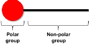
Surfactants are amphiphilic molecules comprising a polar component with affinity for water and a non-polar part that has affinity to non-polar fluids. This double affinity allows surfactants to diffuse to the interface between two phases (oil and water) and to decrease the free energy of the system. The polar part of the surfactant can be charged positively or negatively or can also be uncharged (nonionic) such as in the case like polyethylene oxide chains. The non-polar part is usually a long chain of hydrocarbon units, including aromatic groups [20]. Figure 1.8 shows a schematic representation of a typical surfactant molecule.

Figure 1.8. Schematic representation of a surfactant molecule

Ionic surfactants dissociate when they are dissolved in water. They are sensitive to changes in the ionic strength of the solution and thus some desired properties of the surfactant can be activated by changes in the salinity of the aqueous medium. These surfactants, depending on how they dissociate in water, can be further classified into anionic, cationic and zwitterionic. Figure 1.9 presents three different examples of ionic surfactants

Figure 1.9. Ionic surfactants: (a) sodium dodecylsulfate, (b) cetyl ammoniumbromide and (c) lauryl betaine.

surfactants. They have shown some antimicrobial activity and therefore have been used in antibacterial products for personal hygiene [20].

Zwitterionic surfactants generate both, an anion and a cation when they dissociate in water. They differ from anionic and cationic surfactants because they are not very sensible to electrolytes in water [21], mainly because they are electrically neutral. An example of zwitterionic surfactant is 3-[(3-Cholamidopropyl)dimethylammonio]-1-propanesulfonate, commonly known as CHAPS, which is used in the process of protein purification [22].

Non-ionic surfactants do not dissociate in water. The polar group is usually composed by an alcohol, an ether or an ethylene oxide chain. These surfactants are known for being sensitive to changes in temperature, affecting the affinity they have for water or oil. Examples of non-ionic surfactants are polyoxyethylene (20) sorbitan monooleate (Tween 80), polyoxyethylene (20) sorbitan monolaurate (Tween 20) and sorbitan monoester (Span 80), among others.

1.3.2 Properties of surfactants

keep them away from the oil phase. The product of association of these surfactants is called “micelle”. Figure 1.10 includes a schematic illustration of adsorption and association of

surfactants in water.

Figure 1.10. Adsorption and association of a surfactant.

1.3.3 Microemulsions and emulsions

Microemulsions are thermodynamically stable dispersions of two immiscible liquids (oil and water) displaying optical transparency and having very unique properties such as super-solubilizing ability for both, polar and nonpolar fluids. In order to form a microemulsion, a surfactant or surfactant mixture is required to decrease to ultralow values the interfacial tension between oil and water and promote the spontaneous mixing of the otherwise immiscible phases. Mixing of the phases occurs spontaneously and leads to systems that are thermodynamically stable. They were first described by Winsor in 1954 [23] and in recent years they have been widely applied in different fields where they have had a major impact, including drug delivery, nanoreaction engineering, cosmetics, food and oil, etc.

Different types of microemulsions exist depending on the phase that is dispersed and the one that is continuous. Direct microemulsions are those where water is the continuous phase and drops of oil are dispersed while reverse microemulsions include water dispersed in the oil, continuous phase. Bi-continuous microemulsions are neither water- nor oil- continuous, instead a microstructure that is bicontinuous is formed (none of the phases can be classified as the continuous or dispersed ones). This is usually the case for systems with similar volumetric fractions of oil and water [24].

therefore, the emulsion will eventually separate into its original constituents. Depending on the formulation, emulsions can be stable for very long periods of time [25].

Emulsions can be classified depending on the nature of the continuous and the dispersed phases. When water is the continuous phase the emulsion is called oil-in-water (O/W). On the other hand, when water is the dispersed phase, the emulsion is called water-in-oil or W/O. It is also possible to have what is called a multiple or double emulsion where the dispersed phase is already and emulsion. These emulsions can be water in oil in water (W/O/W) or oil in water in oil (O/W/O) [25].

1.3.4 Physicochemical models to formulate SOW systems

Different models have been proposed to understand the physicochemical behavior of systems containing surfactant (S), water or an electrolyte solution (W) and an organic phase or oil (O). They differ in complexity and properties evaluated but they all are intended to ease the process of emulsion formulation. The selection of one specific model will depend on the objective of the emulsion formulator. Two different models are introduced next: the Winsor R ratio and the Surfactant Affinity Difference (SAD).

1.3.4.1Winsor R ratio and HLB

𝑅 = 𝐴𝐶𝑂

𝐴𝐶𝑊 Equation 1.1

If R>1, the interactions between the surfactant and the oil phase are stronger than those with water, indicating that the surfactant is relatively lipophilic. The opposite case is obtained when R<1, the surfactant has stronger interactions with water and thus the surfactant, on a relative basis, is hydrophilic. If R=1, the interaction of the surfactant with oil and water are comparable [23]. This model is very useful to explain qualitatively the behavior of a system but it is not applicable when quantitative information is required for the formulation of a system.

The hydrophilic lipophilic balance (HLB) is a very useful model for the characterization of a surfactant. This concept was introduced by Griffin in 1949 and it assigns a number, the HLB to a surfactant based on the stability of an emulsion prepared with the surfactant. The HLB scale goes from 1 to 20 where 1 represents a highly lipophilic and 20 a highly hydrophilic surfactant. The HLB parameter can be used to select a surfactant based on the type of emulsion to be formulated. Figure 1.11 presents possible applications and types of emulsions that can be obtained depending on the HLB values of the surfactant [25].

1.3.4.2Surfactant Affinity Difference (SAD) approach

This approach was proposed by Salager in 1985 [26] who used a parameter that accounts for the differences in the interactions of the surfactant with the given oil and water phases. The difference between this parameter and Winsor R is that SAD provides quantitative information based on empirical equations that use experimentally-derived parameters. Equations 1.2 and 1.3 include the main equations to calculate the SAD value for an ionic and a non-ionic surfactant in contact with given oil and water media, respectively.

𝑆𝐴𝐷

𝑅∙𝑇 = ln(𝑆) + 𝑘 ∙ 𝐸𝐴𝐶𝑁 − 𝑓(𝐴) + 𝜎 − 𝑎𝑇∙ (𝑇 − 25) = 0 Equation 1.2 𝑆𝐴𝐷

𝑅∙𝑇 = 𝛼 − 𝐸𝑂𝑁 − 𝑘 ∙ 𝐸𝐴𝐶𝑁 + ∑(𝑀𝑖𝐴𝑖) + 𝑏𝑆 + 𝑐𝑇∙ (𝑇 − 28) Equation 1.3

where S is the salinity of the aqueous phase (wt. %), k is a parameter that depends on the surfactant type, EACN is the equivalent alkane carbon number of the oil, f(A) is a function that depends on the alcohol type and concentration, σ is a surfactant parameter, aT is a coefficient

with temperature[27]. The SAD and Winsor R values are related since R>1 is equivalent to SAD>1; R<1 is equivalent to SAD<1 and R=1 is equivalent to SAD = 0 [26, 27].

1.3.5 Phase behavior of SOW systems and formulation scans

1.3.5.1Winsor diagrams

Winsor proposed in 1954 [23] the use of ternary diagrams to represent the phase behavior of SOW systems. In the ternary diagram, one apex of the ternary diagram corresponds to the surfactant, and the other two correspond to the oil and water phases, respectively. According to the ideal model of Winsor, three different scenarios can be found when water, oil and a surfactant are mixed together and let to equilibrate. These scenarios are called Winsor I, Winsor II and Winsor III, as represented in figure 1.12.

Figure 1.12. Winsor phase equilibriums for SOW systems

.

the single-phase region above a certain concentration of surfactant and a two-phase region, where the systems separate in a (typically) denser (bottom phase in a test tube) microemulsion phase that is oil-in-water and an upper, excess oil phase. In a Winsor II type system (Fig 1.12c), similar two regions are found: (single and a two-phase regions). The difference here is that the interactions between the surfactant and oil are stronger than the interactions between the surfactant and water (R>1). Therefore the systems in the two-phase region separate into one upper phase that is a water-in-oil microemulsion and an excess water, bottom phase. Finally, for a Winsor III type systems, the interactions between the surfactant and water or oil are balanced (R=1) and three-phase region is found (Fig. 1.12b). The systems in the three-phase region will separate in a middle phase that is a bi-continuous microemulsion and excess oil and water phases. The two-phase regions will separate similar to the Winsor I and II cases [23].

1.3.5.2Formulation scans

surfactant, it is possible to observe a change from a Winsor I type system for low salinity to a Winsor III type system for intermediate salinities and finally a Winsor II system for high salinities. Formulation scans are very helpful to determine the conditions for the formation of a certain type of emulsion or to tune the properties of certain surfactant to produce a given type of emulsion [25].

After the basic concepts regarding surfactant – oil – water systems were introduced, another important topic will be addressed and that is nanocellulose. In the present work, different applications including nanocellulose are presented; therefore the understanding of the process of manufacture will be very beneficial.

Nanocellulose

Nanocellulose is the name given to a material composed by nanosized extracted cellulose fibrils or particles. Two types of nanocelluloses can be considered: cellulose nanocrystals (CNCs) and cellulose nanofibers (CNFs) [28]. Other classifications and names can be found for nanocellulose, including cellulose nanowhiskers, cellulose nano-ribbons and bacterial cellulose; however, this work will be concerned with CNC and CNF.

1.4.1 Cellulose nanocrystals (CNCs)

high mechanical strength [4, 29]. The applications for these nanomaterial are very wide and include reinforcement of nanocomposites, hydrogels, films, coatings, etc. [4, 28-31]

Cellulose nanocrystals can be produced from different cellulosic sources including but not limited to cotton, ramie, tunicate, sisal, wood and bacterial cellulose. Depending on the raw material and the conditions for the hydrolysis, the resulting CNCs could have different morphology. The two most common techniques used for characterization of CNCs are atomic force microscopy (AFM) and transmission electron microscopy (TEM). Figure 1.13 includes CNCs obtained from different raw materials [4] where one can appreciate the differences in size and morphology of the CNCs depending on the raw material used.

CNCs are obtained after removal of the amorphous domains of cellulosic materials via acid hydrolysis. The kinetics of the hydrolysis of the amorphous regions under acid conditions is much faster than the kinetics of hydrolysis of the crystalline parts; therefore, the crystalline part tend to remain almost intact while the amorphous part can be fully hydrolyzed [4, 31].

Different acids have been reported for the production of CNCs. Among the acids sulfuric and hydrochloric acids are the most studied. When the hydrolysis is performed using sulfuric acid, the surface of the crystals is decorated with half-sulfate groups. The conditions reported for the reaction using sulfuric acid include temperatures from 25 to 70 °C, reactions times from 30 minutes to 12 h and concentrations of acid around 65% by weight. Some studies support that the length of the crystals is related to the time of the reaction, deriving in short crystals when the reaction time is long [4, 31]. For the reaction using hydrochloric acid the conditions are different than for the reaction with sulfuric acid. The reported temperatures are slightly higher, around 105 °C and the concentration of the acid is usually between 2.5 to 4N. The reaction times are selected based on the raw material, for instance 20 minutes have been used for cotton as a starting material [4, 32]. A comprehensive study of different conditions for the preparation of CNCs using sulfuric acid is presented by Wang et al.[33] in a recent publication where they studied the kinetics of sulfuric acid hydrolysis for different acid concentrations and temperature.

reason for this difference is the surface charge of the resulting CNCs that is more negative when sulfuric acid is use, due to the presence of half-sulfate groups on the surface of the crystals. In fact, CNCs prepared using hydrochloric acid have very low surface charge [31, 34].

Other methods of preparation of CNCs have been recently reported using different chemicals for hydrolysis of cellulosic materials, for instance, the preparation of spherical CNCs using ammonium persulfate. These spherical crystals are reported to be more reactive, more flexible and easier to process because they have a better thermal stability compared to the CNCs obtained by acid hydrolysis using inorganic acids [35].

1.4.2 Cellulose Nanofibers (CNF)

modification of CNF is usually performed to improve the compatibility of the material with other hydrophobic polymers and enhance the compatibilization in nanocomposites [36, 37]

In order to prepare NFC, a suspension of a cellulosic material in water is subjected to mechanical disintegration that causes the fibrillation of the material to the nanoscale. This procedure usually implies high mechanical energy consumption, which is a drawback of the process. Pretreatment of the raw material is used as an alternative to reduce the energy consumption during the process of fibrillation and is a subject that will be discussed in other chapters of this thesis [36, 38].

Different methods can be followed to fibrillate the original cellulosic material to CNF; however, three techniques are usually preferred for the manufacture of NFC: homogenization, the microfluidization and the microgrinding. In a homogenizer, the suspension of the cellulosic raw material is fibrillated by the action of a pressure change in a pneumatic valve shaft. In the case of the microfluidizer, the suspension is sent through an interaction chamber that is composed by several microchannels where the suspension is under high shear and the fibrillation is attained. Finally, in the microgrinder the suspension is fibrillated using two grinding stones that rotate in countersense and imparts high shear to the cellulosic material [36]. The approximated energy consumption per pass for these units is around 1095 kWh/ton for the homogenizer, 172 kWh/ton for the microgrinder and 175 kWh/ton for the microfluidizer [38].

surface of the fibers in order to reduce the strength of the hydrogen bonding that links together the fibers. Among the mechanical pretreatments the valley beater and the PFI mill pre-treatments are reported; whereas in the chemical pretreatment TEMPO-mediated oxidation and carboxymethylation are the most popular ones [36, 38, 39].

The CNF size and other characteristics are not very dependent on the raw material used, as was the case for CNCs. The final size of the nanofibrils is more related to the conditions used for the fibrillation; specifically the number of passes through the deconstruction unit. Figure 1.14 includes images obtained by scanning electron microscopy of the evolution of the characteristic size as the processing time is increased in a microgrinder [40].

Figure 1.14. Scanning electron microscopy images of nanofibrillation of cellulosic fibers using a microgrinder for 0 hours (A); 0.25 hours (B); 6 hours (C) and 9 hours (D) [40].

[1] Energy Information Administration. Monthly Energy Review, September 2013.

http://www.eia.gov/totalenergy/data/monthly/

[2] S. Naik, V.V. Goud, P.K. Rout, A.K. Dalai, Renewable and Sustainable Energy Reviews. 14 (2010) 578.

[3] R.M. Rowell, The Chemistry of Solid Wood, ACS Publications, 1984.

[4] Y. Habibi, L.A. Lucia, O.J. Rojas, Chem Rev. 110 (2010) 3479.

[5] S. Thomas, Advances in Natural Polymers Composites and Nanocomposites, Springer Berlin Heidelberg, 2013.

[6] I. Mladenovic, C. Weindl, Proceedings International Conference on Clean Electrical Power (2009) 705.

[7] M. Ioelovich, BioResources. 3 (2008) 1403.

[8] T. van de Ven, G. Louis, Cellulose – Medical, Pharmaceutical and Electronic Applications, InTech (2013).

[9] B.C. Saha, Journal of Industrial Microbiology and Biotechnology. 30 (2003) 279.

[10] F.S. Chakar, A.J. Ragauskas, Industrial Crops and Products. 20 (2004) 131.

[12] B. Monties, K. Fukushima, Biopolymers Online. (2001) .

[13] Integrated Biorefineries: Biofuels, Biopower, and Bioproducts, (2013)

https://www1.eere.energy.gov/bioenergy/pdfs/ibr_portfolio_overview.pdf.

[14] M.E. Himmel, S.Y. Ding, D.K. Johnson, W.S. Adney, M.R. Nimlos, J.W. Brady, T.D. Foust, Science. 315 (2007) 804.

[15] B. Yang, C.E. Wyman, Biofuels, Bioproducts and Biorefining. 2 (2008) 26. doi:10.1002/bbb.49.

[16] Z. Bo, Biomass Processing, Conversion, and Biorefinery, Nova Science Publishers, Inc, Hauppauge, New York, 2013.

[17] T. Bui, R. Loof, S. Bhattacharya, Energy. 19 (1994) 397.

[18] C.J. Biermann, Handbook of Pulping and Papermaking, Academic Press, San Diego, (1996).

[19] Annual Report, Mercer International Ink. (2003). http://yahoo.brand.edgar-online.com/EFX_dll/EDGARpro.dll?FetchFilingHTML1?ID=6450076&SessionID=nm71Fv 6dLSFApX7

[20] C. Arun, K.L. Mittal, Surfactants in Solution, Marcel Dekker, New York, (1996).

[22] L.M. Hjelmeland, Nondenaturing zwitterionic detergents. (1983) .

[23] P. Winsor (Ed.), Solvent Properties of Amphiphilic Compounds, Butterworths Scientific Publications, London, (1954).

[24] C. Stubenrauch (Ed.), Microemulsions, Blackwell Publishing Ltd, United Kingdom, (2009).

[25] B. Paul, Encyclopedia of Emulsion Technology, M. Dekker, New York, (1983).

[26] J. Salager, Proceedings, 1st International Symposium Enhanced Oil Recovery (1985).

[27] J. Salager, Progr Colloid Polym Sci. 100 (1996) 137.

[28] A. Dufresne, Nanocellulose: From Nature to High Performance Tailored Materials, Walter de Gruyter, (2012).

[29] S. Eichhorn, A. Dufresne, M. Aranguren, N. Marcovich, J. Capadona, S. Rowan, C. Weder, W. Thielemans, M. Roman, S. Renneckar, J Mater Sci. 45 (2010) 1.

[30] X. Qiu, S. Hu, Materials. 6 (2013) 738.

[31] S.J. Eichhorn, Soft Matter. 7 (2011) 303.

[32] B. Braun, J.R. Dorgan, J.P. Chandler, Biomacromolecules. 9 (2008) 1255.

[34] Azizi Samir, My Ahmed Said, F. Alloin, A. Dufresne, Biomacromolecules. 6 (2005) 612.

[35] M. Cheng, Z. Qin, Y. Liu, Y. Qin, T. Li, L. Chen, M. Zhu, Journal of Materials Chemistry A. 2 (2014) 251.

[36] K. Missoum, M.N. Belgacem, J. Bras, Materials. 6 (2013) 1745.

[37] I. Siró, D. Plackett, Cellulose. 17 (2010) 459.

[38] K.L. Spence, R.A. Venditti, O.J. Rojas, Y. Habibi, J.J. Pawlak, Cellulose. 18 (2011) 1097.

[39] T. Saito, Y. Nishiyama, J. Putaux, M. Vignon, A. Isogai, Biomacromolecules. 7 (2006) 1687.

2

Research Objectives

The general objective of this work is to introduce multiphase systems consisting of oil and aqueous phases stabilized by surfactants or particles, generally classified as “complex fluids”, in different processes involving lignocellulosic biomass. Complex fluids can be used

in different applications including but not limited to:

a. Improved impregnation of woody biomass as pretreatment for bioethanol production, wood preservation, chemical modification and surface finishing.

b. Enhanced chemical delivery using microemulsions as carrier of active agents into the capillary structure of lignocellulosic biomass, for example for derivatization or fractionation.

c. Advanced compatibilization of lignocellulosic and its derivatives.

d. Chemical modification of lignocellulosic biomass via emulsions or microemulsions droplets used as nano or micro reactors.

3

Capillary Flooding of Wood with Microemulsions from Winsor I

systems

Carrillo et al. Journal of Colloids and Interface Science. 381 (2012) 171-179

Abstract

A new approach based on microemulsions formulated with at least 85 % water and minority components consisting of oil (limonene) and surfactant (anionic and nonionic) is demonstrated for the effective flooding of wood’s complex capillary structure. The formulation

Introduction

The main challenge for effective fluid penetration in solids with complex structures is overcoming the capillary forces to facilitate the displacement of air from any void spaces present in the system. A typical example is that of wood where impregnation using fluids has been implemented for biocide delivery[1], hydrophobization[2], preservation[3] and surface modification[4, 5]. Typically, severe pressure changes and high temperatures are used in the disruption of the capillary structure of solids with fluids. In the case of wood, first vacuum is applied for the removal of air, followed by high pressure impregnation to force the penetration of the given liquid [1, 6]. The required operating pressure and the need for high strength materials are associated with high capital and operating costs. An attractive option is therefore the replacement of mechanical (pressure) and thermal energies by chemical energy, such that the cost, resource usage and safety risks associated with high pressure operations are minimized.

economically-efficient technologies. Thus, the improvement of biomass impregnation by using new, environmentally friendly approaches forms the core of our interest.

A scenario similar to that of wood impregnation is found in the field of enhanced oil recovery, for example, in injection of fluids, flooding of crude oil reservoirs with displacers, etc. In such cases fluid penetration into the void spaces is required to displace the oil trapped in the mineral formation. The best results for oil recovery have been achieved by the use of complex fluids, including microemulsions [9-12]. The term “microemulsion” implies systems with micron-size droplets. However, in agreement with the general usage, in this work it is meant to indicate emulsions that are spontaneously formed, are thermodynamically stable, and may involve bicontinuous structures composed of oil and water. This is in contrast to other type of emulsions, such a macro- or nano-emulsions, which require the addition of energy for emulsification and stabilization of the formed droplets in the continuous phase [13-16]. Among the unique characteristics that make microemulsions effective in, for example, oil recovery is their ultralow interfacial tension and also the suitable viscosity for displacement of oil.

We formulated simple Surfactant-Oil-Water (SOW) systems to penetrate wood and fill its void spaces at atmospheric pressure and room temperature. Phase behavior scans of SOW systems were carried out, and after identification of a balanced “surfactant affinity difference”[20], microemulsions derived from the so-called Winsor I systems[21] were

applied. Proof-of-concept impregnation experiments were carried out by using a commercial anionic and a nonionic surfactant together with a natural oil, all of which were minority components in the microemulsions. The ability of microemulsions to solubilize both water- and oil- soluble components of the cell wall was also explored. Overall, microemulsions are proposed as an alternative to advance the field of solid impregnation, especially relevant in biomass pretreatment technologies.

Experimental section

3.3.1 Materials and Methods

determined by using a rheometer from TA Instruments, model AR2000. The mixing system consisted of a Precision Stirrer of variable speed from Glas-Col, Terre Haute. For measurement of surface tension and impregnation rates, a 312 Electrobalance from Cahn Instruments Inc. (California) equipped with a platinum Wilhelmy plate was used. Solids content before and after wood impregnation with the tested fluids (microemulsions and base fluids) was determined with a HB43 Halogen Moisture Analyzer from Mettler Toledo (Switzerland).

3.3.2 Equivalent alkane carbon number (EACN) of limonene.

The rationale for the selection of the surfactant system was based on the equivalent alkane carbon number (EACN) of the organic phase, i.e., limonene (O). The EACN of limonene was determined by using the double salinity SOW scan technique and details about this procedure, calculation and related references are provided in the Supporting Information document. EACN of 8.2 was determined for the limonene sample used in this investigation and therefore, as a first attempt to study the proposed microemulsion systems, sodium dodecyl sulfate was chosen as base surfactant. This is based on the observation that SDS is known as a good emulsifier for organic phases of similar EACNs (for example, n-octane). Additionally, a mixture of SDS with the nonionic surfactant was employed in order to test possible synergies in surface activity.

3.3.3 Phase behavior of SOW systems.

SOW system contained an anionic surfactant, SDS, at 2 g/dL concentration based on total volume. The water-to-oil ratio (WOR) was 1 and the alcohol used was n-pentanol at a concentration of 5% v/v based on the total volume. The electrolyte used was sodium chloride at a concentration that ranged from 1.2 to 6.8% in weight based on the volume of the aqueous phase. An additional SOW system was used in similar scans as those performed in the case of single (SDS) surfactant. It consisted of a binary surfactant, i.e., a 2:1 mixture of (anionic) SDS and (nonionic) polyoxyethylene sorbitan monooleate (Tween 80), at a total concentration of 3 % based on the SOW volume. All the SOW systems were left to reach equilibrium at room temperature, and the type of Winsor system was identified [21]. The volume fraction of each phase separated was measured at the given salt concentration (salinity).

3.3.4 Pseudo-ternary phase diagram.

3.3.5 SOW emulsification.

In order to formulate microemulsions with a high WOR (water-to-oil ratio) Winsor type I systems were chosen from the salinity scans, and the approximate compositions of the microemulsion were obtained. Accurate component inventory of the respective stable, one-phase microemulsion was determined by the titration method by using different amounts of surfactant and alcohol [22, 23]. Four different microemulsions were tested in further impregnation experiments: two involving a single surfactant (SDS) and the other two with a binary mixture (with the anionic, SDS and, the nonionic surfactant). Additional formulations were used to test the effect of fluid physical properties on fluid penetration.

3.3.6 Wood samples and rate of fluid penetration.

The wood samples consisted of eastern white pine (Pinus strobus) at an equilibrium moisture content of 5.8 % first cut (circular saw) in the axial direction (along the grain) that were used as blocks having 6.1 × 13.2 mm cross sectional area. Then, smaller parallelepipeds (20.5 × 6.1 × 13.2 mm) were cut using a bandsaw (cut across the grain).

To determine the liquid uptake by the wood samples, two different tests were performed: “wicking” by the solid sample upon contact of one side with the impregnation fluid and “full immersion”. In typical wicking experiments, one side of the wood sample hung on a wire (with

the axial or fiber direction perpendicular to the fluid surface) and was positioned 3 mm below the fluid surface. The weight gain after contact, due to liquid uptake, was monitored every second during a total period of 4 hours (by using the Cahn 312 microbalance). Thus, uniaxial fluid penetration into the wood samples was measured. The positioning of the wood samples was chosen to facilitate the faster impregnation in the axial direction compared to those in the tangential or cross directions [24, 25].

(volume of solid fraction, etc.) the samples were always returned to the impregnation vessel after measurement.

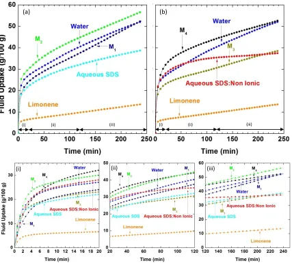
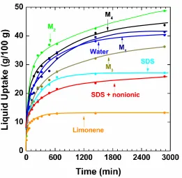
Four microemulsions were tested and compared against the base fluids (water, limonene and aqueous solutions of the surfactants) which were used as reference in the quantification of the dynamics and extent of solid impregnation. The amount of liquid uptake was normalized by the mass of the wood sample and used to construct impregnation isotherms as a function of contact time.

3.3.7 Influence of WOR in the properties of the microemulsions.

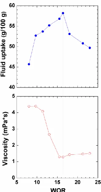
In addition to the two main microemulsion systems, seven microemulsions of increasing water-to-oil ratio (WOR) ratio, from 8 to 23, were prepared following the procedure described before. These microemulsions were used to test the effect of WOR in wood impregnation. The viscosity and liquid uptake by wood (after 4 hours contact time) were determined as a function of the WOR.

3.3.8 Solubilization of components of wood cell walls.

extracted wood was then dried and hydrolyzed with H2SO4 (72% by weight) during 2 hours with stirring every 15 minutes. The hydrolyzed mixture was processed further for determination of lignin (UV-Vis, 205 nm) and carbohydrate content and distribution (HPLC, Agilent, Santa Clara, CA. USA).

Results and discussion

3.4.1 SOW Phase Behavior.

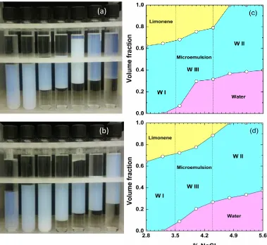
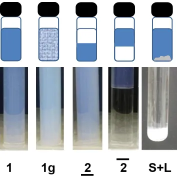
A justification for the use of SDS as surface active molecule is provided as Supporting Information along with the determination of the EACN of the limonene (O phase). The phase behavior of systems involving SDS and also SDS mixed with the nonionic surfactant was studied. Figure 3.1a, b shows salinity scans with increased salt concentration (from left to right) in the tests tubes that contain the respective SOW system. The height (or volume fraction) of the phase separated in each case was measured and plotted against the salinity of the aqueous phase. As a result, Figure 3.1c and 3.1d show the calculated volume fraction as a function of the salinity of the aqueous phase for systems based on SDS and SDS mixed with the nonionic surfactant, respectively.

For intermediate salinities the affinity of the surfactant is balanced for both, water and oil, and Winsor III type systems are obtained. These systems have three different phases, the middle, microemulsion phase and a bottom and upper phases with excess water and excess oil,

Figure 3.1. Phase separation from salinity scans in SOW systems consisting of water (W) and limonene (O) with SDS (a) or SDS: noinionic surfactant (2:1) (b). For both systems the water-to-oil ratio (WOR) was 1 and n-pentanol was used as co-surfactant (5% v/v). The salinity values in the test tubes, from left to right, corresponded to 2.8, 3.2, 3.6, 4.0, 4.4, 4.8 and 5.2 g/dL. Winsor transitions observed as a function of the location of the surfactant between the aqueous and the organic phases (lower and upper phases in the respective test tube) correspond to Winsor I (surfactant located in the turbid, aqueous phase), Winsor III (surfactant located in the middle phase) and Winsor II (surfactant located in the organic phase). The right panels show the phase diagrams as volume fraction of each phase as a function of salinity (“c” and “d” for the respective systems).

(a)

respectively. The optimum salinities (as commonly referred for Winsor III systems) were 3.8 and 4.2 % NaCl for the SOW mixtures with SDS and the surfactant mixture, respectively. At high salinities the surfactant becomes less soluble in water and it is salted out in the oil phase, whereupon a Winsor II type system is obtained. These two-phase, Winsor II systems include the microemulsion, upper phase which contains all the oil and the lower phase or excess water. It can be observed that addition of the nonionic surfactant increased the amount of microemulsion phase obtained, especially for the Winsor III type systems. This fact can be explained by the synergistic effect in surfactant mixture, as has been reported in other studies [26-28].

Overall, the information obtained from the salinity scans is critical to evaluate the influence of the ionic strength of the aqueous phase on surfactant affinity. Because our main goal was to obtain microemulsions with high WOR, salinities corresponding to Winsor I type systems were selected and investigated further.

3.4.2 Pseudo-ternary phase diagram.

location of the single-phase zone in the pseudo ternary diagram is critical for successfully formulating the microemulsions. The loci of each region in the pseudo-ternary diagram are depicted in Figure 3.2. M1 and M2 represent a single phase microemulsion systems and S1 a pseudo surfactant aqueous solution. M1 and M2 microemulsions are formulated so as to contain the same surfactant concentration, but different WOR (M2 has more water, higher WOR than M1), as indicated in the inset of ternary diagram in Figure 3.2.

Figure 3.2: Left: Pseudo-ternary phase diagram for the SOW system with single surfactant: water (3.2% w NaCl) (W) – limonene (O) – surfactant solution (S) (8% w SDS in 3.2% w NaCl and 5% v/v n-pentanol). Right: Pseudo-ternary phase diagram for the SOW system with bicomponent surfactant: water (2.8% w NaCl) (W) – limonene (O) – surfactant solution (S) (8% w SDS and 4% w Tween 80 in 2.8% w NaCl and 5% v/v n-pentanol). The ternary diagrams were obtained at room temperature. The upper and lower bars on numeral “2” indicate the locations of the surfactant in the two-phase systems (lower and upper phases for 2- underscored and 2-upperscore, respectively (see also Figure 1 as a reference)). The “1” in the middle phase indicates single phase SOW systems. The “1g” indicates a monophasic, gel-type system. The inset (center) with a magnified view represents the composition loci of M1 and M2 microemulsion systems in the pseudo-ternary diagram for the single surfactant SOW system (left).

S1 represents an aqueous solution containing only the surfactant and the respective amount of salt (no oil). The preparation of the microemulsions was carried out by adding first the surfactant aqueous solution, then the electrolyte solution, followed by oil and finally the co-surfactant. The microemulsions were prepared under continuous stirring using a constant shear rate, equivalent to 400 rpm. Similar approaches (ternary diagram and formulation, mixing protocol, etc.) apply to the case of microemulsions based on SDS-nonionic surfactant mixture, named thereafter M3 and M4 (data not shown).

For the pseudo-ternary based on the anionic SDS surfactant at low concentrations the SOW system comprised two coexisting phases (2 lower-score in Fig. 3.2) with an upper, excess oil phase and a bottom, microemulsion phase (containing all the water of the system). The single phase region (1 in Fig. 3.2) is located at intermediate surfactant concentrations. Under these conditions, the only phase present in the system is a microemulsion containing all the components. This microemulsion is stable and is formed spontaneously after low energy mixing. At the highest surfactant concentration, a two-phase region (2-upper score in Figure 3.2) is found again, but it comprises an upper, microemulsion phase containing all the limonene and a bottom, excess water phase.

the 10% limonene line, the WOR and the electrolyte concentration is constant; thus, the phase transitions crossed by the line are due to the change in the surfactant/co-surfactant concentration in the system. The concentration of the surfactant/cosurfactant mixture increases as the composition is moved to the top of the diagram following the 10% limonene line. In addition, the presence of alcohol makes the mixtures more lipophilic (the alcohol used is relatively lipophilic). The microemulsions in 2-lower score systems (for low surfactant/co-surfactant concentrations) consist of normal micelles (micelles with the lipophilic tails of the surfactant in the core) while the opposite is expected at high surfactant concentration whereby inverse micelles are expected due to the increase in the lipophilicity of the mixture. Bi-continuous structures are expected to exist at intermediate concentrations.

A similar behavior as that observed for SOW systems with pure SDS occurs in the case of systems consisting of a binary surfactant mixture (SDS and Tween80), as indicated in the respective SOW pseudo-ternary diagram (Figure 3.2). The different phase zones are observed, two single-phase (1 and 1g) and one two-phase (2 lower score). The presence of the 1g gel zone suggests self-organization of the surfactant molecules which results in an increased viscosity of the system. This behavior has been reported [30] and can be ascribed as the result of interactions of the charged head groups of SDS and the n-pentanol and/or the nonionic surfactant present in highly concentrated systems. As the concentration of the surfactant mixture decreases a phase behavior similar to that observed for the pure SDS system takes place.

aqueous phase. The single-phase systems studied here are located in the area of the ternary diagram located between 60 to 70% surfactant aqueous solution concentrations. This information allows narrowing the concentration of the components for the preparation of the microemulsions, reducing considerably the experimental work.

3.4.3 Microemulsions: formulation, emulsification and properties.

The composition of the microemulsion in each test tube of Figure 3.1 was calculated by assuming that the excess phase (O or W) was neat, depending on the Winsor system type. For example, for Winsor I SOW systems the excess phase (upper, O phase) was assumed to be pure limonene. Noting that in Winsor I type systems the assumption made in the calculation of SOW composition applies better than in the case of Winsor II or III systems. This is because all the water and NaCl are present in the microemulsion phase of Winsor I SOW systems (lower phase in the test tubes of Figure 3.1a,b). For Winsor II or III systems some salt and surfactant remains solubilized in the lower, aqueous phase. The calculated compositions were used to experimentally reproduce the respective microemulsion composition using the titration method. The calculated values for the surfactant concentration for the SDS microemulsions belong to the range of values obtained with the pseudo-ternary diagram.

the salinity scans. However, the final formulation (and composition) to obtain single-phase, thermodynamically-stable microemulsions with high water content (M1, M2, M3 and M4) was experimentally adjusted by using the titration method. For this purpose the water, the surfactant solution, the electrolyte and the oil phases were mixed and then the co-surfactant was slowly added until the system became optically clear [22, 23].

For systems involving SDS as surfactant (M1 and M2), the salinity was selected to be 0.0236 g/mL (based on total microemulsion volume). M1 and M2 contained the same concentration of NaCl and SDS but different WOR. For the system using the mixed surfactant (anionic SDS and nonionic polyoxyethylene sorbitan monooleate), M3 and M4, the salinity selected was 0.0208 g/mL. M3 and M4 have the same NaCl and surfactant content but different WOR. The final amounts of each component of the microemulsions are presented in Table 3.1.

Table 3.1: Composition1 of the four microemulsions formulated after the salinity scans and titration. M1 and M2 used anionic (SDS) surfactant and M3 and M4 used the surfactant mixture (anionic + nonionic). Microemulsions M1, M2, M3 and M4 are monophasic systems at room temperature.

M1 M2 M3 M4

Anionic SDS (g) 4.9 4.9 6.9 6.9

Nonionic Surfactant (g) -- -- 3.5 3.5

NaCl (g) 2.3 2.3 2.0 2.0

1-pentanol (ml) 3.4 2.7 3.9 2.4

Water (ml) 87.6 91.5 87.2 91.7

Oil (ml) 9.0 5.9 9.0 5.9

WOR 9.7 15.5 9.7 15.5

A schematic representation of the composition loci of microemulsions M1 and M2 in the pseudo-ternary diagram of the SOW system is shown in the inset of Figure 3.2. The WOR increases as the composition of a given system is moved towards that of an oil-free system, for example from M1 to S1 (with S1 an aqueous solution of the surfactant on the S-W line).

Fluid flow in capillary networks has been addressed, for example, in the work of Washburn (Lucas and Washburn equation)[31]. The viscosity and the surface tension of the impregnating fluid, in our case the microemulsions, are expected to be directly related with the distance that the fluid can reach inside the porous media. Therefore, surface tension, viscosity and density of the four microemulsions obtained as well as those of the neat phases (water and oil) are listed in Table 3.2. The microemulsion viscosity and surface tension changed considerably from one system to the other. The viscosity decreased as the WOR increased (from M1 to M2 or from M3 to M4). This is explained by the reduced amount of oil and the lower molecular friction [32]. The increase in surface tension observed with the water fraction in the microemulsion is also as expected [33]: the amount of oil is smaller in M2 or M4, which is the component with the lower surface tension.

Table 3.2: Physical properties of microemulsions measured at room temperature.

M1 M2 M3 M4 Water Limonene

Density (Kg/m3_{) 10 1024 1066 1040 1008 846}

Viscosity (mPa*s) 4.4 1.3 8.3 2.6 1.04 0.94