ABSTRACT
PESANTEZ SARMIENTO, JORGE EDUARDO. A Multi-Step Simulation-Optimization Approach to Design District Metering Areas for Water Distribution Networks. (Under the direction of Dr. Gnanamanikam Mahinthakumar and Dr. Emily Berglund).
A Multi-Step Simulation-Optimization Approach to Designing District Metering Areas for Water Distribution Networks
by
Jorge Eduardo Pesantez Sarmiento
A thesis submitted to the Graduate Faculty of North Carolina State University
in partial fulfillment of the requirements for the degree of
Master of Science
Civil Engineering
Raleigh, North Carolina 2017
APPROVED BY:
_______________________________ Dr. Earl Brill
Committee Member
_______________________________ _______________________________ Dr. Gnanamanikam Mahinthakumar Dr. Emily Berglund
DEDICATION
iii BIOGRAPHY
ACKNOWLEDGMENTS
v TABLE OF CONTENTS
LIST OF TABLES ... vii
LIST OF FIGURES ... viii
CHAPTER 1: INTRODUCTION ... 1
CHAPTER 2: BACKGROUND ... 5
CHAPTER 3: METHODOLOGY ... 7
3.1 Method Overview... 7
3.2 Preliminary Analysis ... 9
3.2.1 Weighting the nodal distance ... 10
3.2.1.1 Hanoi Network ... 11
3.2.1.2 C-Town Network ... 12
3.2.1.3 Micropolis Network ... 12
3.2.1.4 E-Town Network ... 13
3.3 Initial DMA Configuration ... 14
3.4 KMCA Algorithm and Number of DMAs ... 19
3.5 Optimization of Coefficients ... 22
3.5.1 Objective Function ... 23
3.5.2 Pattern Search Algorithm ... 24
3.6 Optimal DMA Configuration ... 25
3.7 Swapping Nodes Process ... 30
3.8 Analysis of Constraints ... 34
3.8.2 Entrances to DMAs Constraints ... 35
3.8.3 Water Level of the Tanks ... 35
3.9 Algorithm Overview ... 35
CHAPTER 4: RESULTS AND DISCUSSION ... 38
4.1 Hanoi Network ... 38
4.2 C-Town Network ... 40
4.3 Micropolis Network ... 42
4.4 E-Town Network ... 44
4.5 Hydraulic Constraints ... 46
CHAPTER 5: CONCLUSIONS ... 51
vii LIST OF TABLES
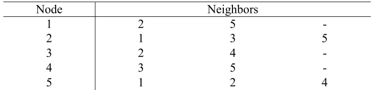
Table 1. Neighbor’s matrix example ... 10
Table 2. Number of DMAs ... 20
Table 3. Known Interior Border Nodes and their Connections ... 27
Table 4. Border Matrix ... 28
Table 5. Connection Matrix example... 30
Table 6. Hanoi results ... 38
Table 7. C-Town results ... 40
Table 8. Micropolis results ... 42
Table 9 E-Town results ... 44
Table 10. Hanoi results of constraints... 46
Table 11. C-Town results of constraints ... 47
Table 12. Micropolis results of constraints ... 47
Table 13. E-Town results of constraints ... 48
LIST OF FIGURES
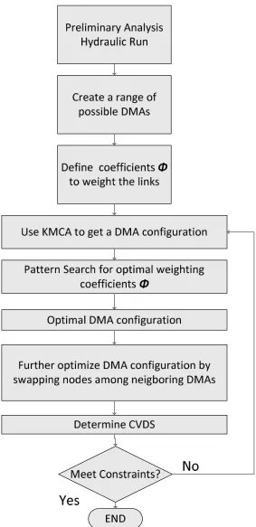
Figure 1. Flow Chart of the Proposed Methodology ... 8
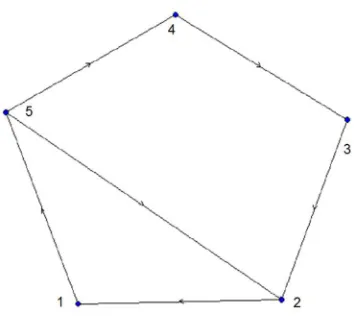
Figure 2. Loop network... 9
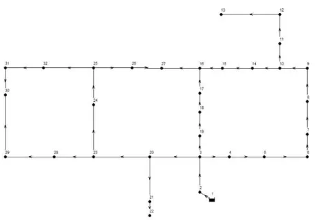
Figure 3. Hanoi Network ... 11
Figure 4. C-Town Network ... 12
Figure 5. Micropolis Network... 13
Figure 6. E-Town network ... 14
Figure 7. Hanoi Network CVDS ... 15
Figure 8. C-Town Network CVDS ... 16
Figure 9. Micropolis Network CVDS ... 16
Figure 10. E-Town Network CVDS ... 17
Figure 11. First phase of KMCA algorithm ... 21
Figure 12. Centroid movement within the clusters ... 22
Figure 13. Descriptive Flow Diagram for Pattern Search ... 25
Figure 14. Interior Border Nodes (IBN) ... 27
Figure 15. Illustration of Heuristic Swapping Process for Improving CVDS of DMAs ... 32
Figure 16. Total Demand of Hanoi for 3 DMAs ... 39
Figure 17. Best DMA configuration for Hanoi ... 39
Figure 18. Total Demand in C-Town for 7 DMAs ... 41
Figure 19. Best DMA configuration for C-Town ... 41
Figure 20. Total Demand in Micropolis for 3 DMAs ... 43
CHAPTER 1: INTRODUCTION
Water Distribution Systems (WDS) are defined as networks comprised of interconnected elements with the main objective of conveying potable water from drinking water treatment plants to service connections within a prescribed area. Those elements are physical components such as junctions, pipes, valves, tanks, and pumps, and each of them represent and meet required conditions regarding hydraulic and quality constraints (Rossman, 2000). Designing a water distribution system depends on several factors, and the challenges of each design criterion are related to three important considerations. First, the diversity of areas where WDS need to be constructed; second, the complexity of finding reliable water sources; and third, the variability in demands (i.e., consumption) that depends on social, cultural and weather conditions throughout the design period. Different types of demands depending on the final usage of water bring another constraint into the design process: residential, commercial and industrial uses have different patterns of consumption that have to be effectively supplied by the WDS. For most of the cases, systems are designed considering parameters including future projected population, peak demand hours, demand patterns, and maximum and minimum pressure in the non-zero demand nodes of the network. Once systems are working, their performance and efficiency are evaluated by the utilities to ensure their quality of service while minimizing costs of operation and maintenance (US EPA, 2006).
more reliable leakage control. The partition of the network produces sub sectors called District Meter Areas (DMAs), which are isolated controlled zones with defined number of entrances and exits (in the case in which a DMA feeds another DMA downstream) that substantially improve the management of a WDS (Grayman, Murray, & Savic, 2009).
of water leaving the treatment plant and the volume measured by micrometers, working together with real time capturing data systems (Smyth & Garandza, 1994) are the common sources to identify the final destination of produced drinking water. On the other hand, the DMA approach provides an advantage to the management of WDS regarding leakage detection, because a straightforward process that requires the difference in volume for each DMA will identify outliers as possible indicators of leaks presence. Once those values and their respective DMA are identified, water utility managers can improve the efficiency of finding leakage spots within a water distribution system (Murray et al., 2009)
This research presents an automatic approach based on graph theory, engineering optimization and heuristic methodology to design District Metering Areas (DMAs) for Water Distribution Systems to determine and redefine the clusters of nodes by minimizing the coefficient of variation of demand similarity (CVDS) among DMAs, and meeting constraints regarding the number of entrances of each DMA, the maximum and minimum pressure at non-zero demand nodes, and maintaining water levels of the tanks over different extended periods of simulation (EPS).
CHAPTER 2: BACKGROUND
Designing a DMA configuration for water distribution systems has been a challenging task, usually carried out by trial and error approaches, and experienced knowledge. Some authors have provided valid methods and results, but depending on the variable to be determined and optimized for each water distribution system there are several outputs that can be taken as local optimal solutions. The DMA’s size, number of boundaries, demand similarity, pressure uniformity, cost of intervention, water quality, among others are some of the factors used to define the objective function to search a good result evaluating numerous generated solutions.
Alvisi & Franchini (2014), presented a procedure using graph theory, specifically Breadth First Search (BFS) and Dijkstra’s algorithm looking for the automatic creation of DMAs, then hydraulic simulations were run in order to get the parameters to satisfy the constraint in terms of the system’s resilience as proposed by Todini (2000). The solution corresponded to the lowest resilience value obtained after the partitioning process.
Water network sectorization concept was introduced by Alcocer-Yamanaka, Di Nardo, Santonastaso, Tzatchkov, & Di Natale (2014), where each district in the system is completely separated or isolated from all other districts, defining isolated iDMAs, with the application of Depth First Search (DFS) algorithm and minimizing an objective function in terms of energy criteria with the use of Genetic Algorithm (GA).
Recently, Scarpa, Lobba, & Becciu (2016), developed an elementary DMA design of looped WDS with multiple sources, based on the concepts of influence area of a supply source to decompose an existing network into isolated subsystems with independent input sources called elementary districts (eDMAs). Once the eDMAs were identified a progressive union constrained by the size of the districts and by a criterion of resilience maximization was performed. Given as a result a set of eDMAs without having an open shared link between each other.
CHAPTER 3: METHODOLOGY
3.1 Method Overview
3.2 Preliminary Analysis
In order to perform a successful analysis in the design of DMAs configuration for a water distribution system, the proposed methodology requires the following input data:
The hydraulic and quality model of the water distribution system Number of DMAs
The minimum and maximum pressure values for non-zero demand nodes Once the input data is retrieved, a spreadsheet with the following information is created:
List of links defined by their pair of nodes Nodal coordinates
Table 1. Neighbor’s matrix example
Node Neighbors
1 2 5 -
2 1 3 5
3 2 4 -
4 3 5 -
5 1 2 4
Table 1 presents the neighbors matrix of a small loop of pipes shown in Figure 2, all the columns of the matrix represent a direct connection with all the nodes of the network. Direction of the flow does not affect neighbor’s matrix because it was created considering only the topology of the network.
3.2.1 Weighting the nodal distance
Water distribution systems can be represented by a weighted graph in which the distance between two nodes is not necessarily the Euclidean distance. Edges representing the links can be assigned a value depending on the type of clustering desired for the DMA. Some good results minimizing the number of links between DMAs were achieved by Paola et al., (2014), by weighting the edges (lij) of the network based on:
Water demand at each node i and node j of link lij,
Vertical distance (difference in elevation) between nodes.
In this research, a combination of parameters is used to weight the graph that represents a water distribution system. To determine which parameters should be considered in the weighting process, an analysis was performed using four networks of different sizes:
Hanoi (Fujiwara & Khang, 1990), C-Town (Salomons, 2009),
Micropolis (Brumbelow, Torres, Guikema, Bristow, & Kanta, 2007), and E-Town (real network), (Saldarriaga et al., 2016).
3.2.1.1 Hanoi Network
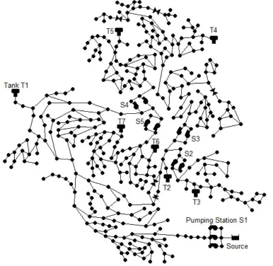
Hanoi network is comprised of 31 junctions, 1 reservoir, 34 pipes, and 3 loops, and represents a small part of the water distribution system of Hanoi, Vietnam. The system works by gravity and is represented by EPANET with a steady state simulation without changes in the demand patterns and it is shown in Figure 3.
3.2.1.2 C-Town Network
C-Town network was presented in the Battle of the Water Calibration Networks (BWCN, 2009), the system is comprised of 388 junctions, 1 reservoir, 7 tanks, 429 pipes, 11 pumps and 4 valves. C-Town represents a medium size network and is presented in Figure 4.
Figure 4. C-Town Network
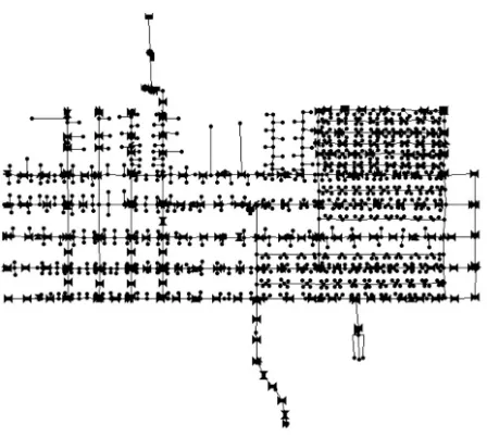
3.2.1.3 Micropolis Network
Figure 5. Micropolis Network
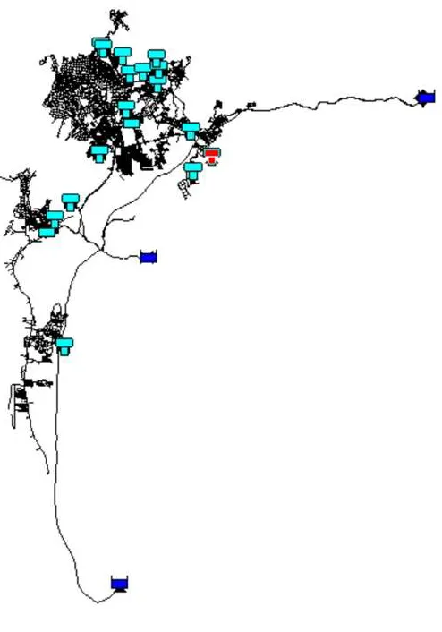
3.2.1.4 E-Town Network
Figure 6. E-Town network
3.3 Initial DMA Configuration
To obtain a low value of the demand’s variance among DMAs and generate possible DMAs configuration, the analysis started evaluating the individual performances of the following parameters:
Diameter (d) Length (l) Flow (flow)
Pressure (p)
Hydraulic Head: elevation + pressure, and Water demand (q)
To get the values of the listed parameters, the present methodology used the EPANET toolkit by running the models with extended periods of simulation varying between 24 and 168 hours.
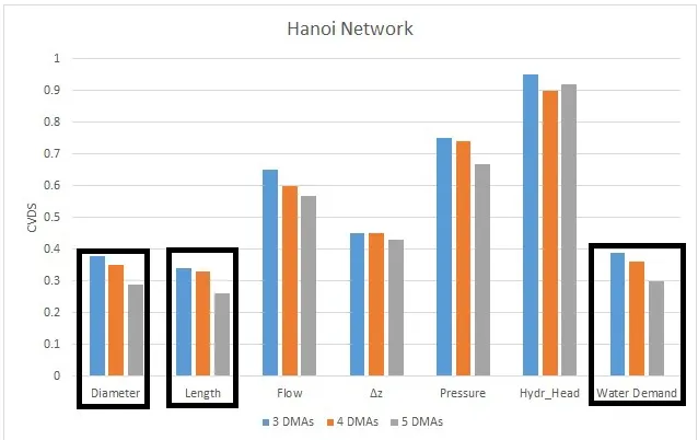
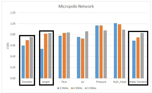
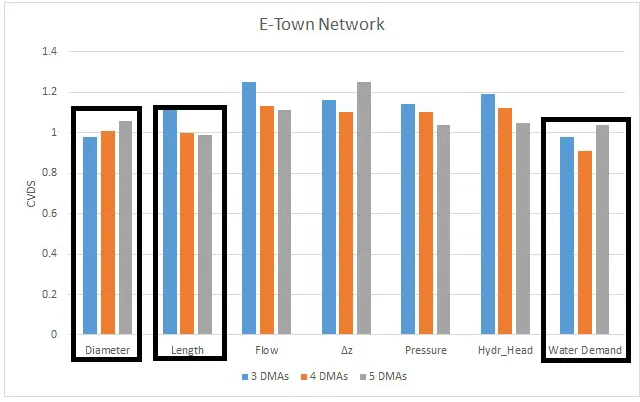
A significant number of trials for all the networks using the mentioned parameters to weight the links of the system and calculate the Coefficient of Variation of demand between DMAs, produced the results shown in Figure 7 to Figure 10.
Figure 8. C-Town Network CVDS
Figure 10. E-Town Network CVDS
Based on the analyzes shown through Figure 7 to Figure 10, a pattern was identified, the lower coefficients of variation specifically in terms of water demand, were generated by weighting the links of the systems with diameter, length and water demand. Between those three parameters, it was not possible to estimate which one was the best at all simulations because they usually switched the order, but still diameter, length and demand generated the lowest values of CVDS.
Therefore, using the mentioned parameters to weight the graph, the metric of each link of the network was represented as established by Equation (1):
1. 2. 3.
k k k k
w d f Q (1)
Where:
wk: metric weight of the links of the system.
fk: normalized flow of water through link k.
Qk: represents the demand existing between nodes i and j that determine link k.
As ϕ, is a set of three weighting parameters, the range of variation of ϕ values was
constrained by the condition that 3
1 1 i i
.To apply Equation (1), the parameters were normalized to make them dimensionless: the diameters of each link were divided by their average value:
( ) k k diam d mean diam
(2)
The flows of each link were divided by the average of their absolute value:
k k
flow f
mean flow
(3)
Finally, the demand Q of a node was divided by the number of edges connected to that node to determine how demand nodes influence the weighting process and then, the demand was normalized dividing the value by the maximum demand value between nodes i and j.
max( ) j i i j k ij dem dem n n Q dem
(4)
Where, dem represents the demand at nodes i and j, and n represents the number of connections that nodes i and j have, respectively. (Paola et al., 2014).
Based on the topology of the network, a water distribution system can be represented by an undirected graph (direction does not count, a link k can be defined by nodes i and j and the link is the same if defined by nodes j and i.), and the adjacency matrix of an undirected graph is a symmetric matrix (Sedgewick & Wayne, 2011).
Once the adjacency matrix was obtained, the Johnson’s algorithm to find all shortest path between nodes in a graph was performed (Johnson & B., 1977). The fact that Johnson’s algorithm works with sparse matrix improved the computing time significantly since water distribution systems are typically represented by sparse graphs.
3.4 KMCA Algorithm and Number of DMAs
To determine an initial configuration of District Metering Areas (DMAs), the weighted graph of the system, and the required number of DMAs are necessary to apply the K-Means Clustering Algorithm (Kanungo et al., 2002).
Regarding the number of DMAs, the proposed methodology generated a range of possibilities based on DMA size, and considering 500 customer connections as the minimum and 5000 as the maximum number of customer connections per DMA (Becciu, Savic, & Ferrari, 2014). Then, the approximate number of customer connections of each system was determined applying Equation (5):
_ #
_ _
syst flow conn
dem per cap
(5)
dem_per_cap: demand per capita that depends on the location of the water distribution system and the final usage of water (residential, commercial or industrial).
The ranges of analyzed DMAs were determined for all the described water distribution systems and are presented in Table 2.
Table 2. Number of DMAs
WDS Number of Customer Connections
Min Number of DMAs
Max Number of DMAs
Hanoi* 252,850 50 500
C-Town 25,334 3 50
Micropolis* 164,377 33 333
E-Town 93,024 18 186
* In order to compare performances, Hanoi and Micropolis were also considered as networks evaluated with 3 DMAs as a minimum value.
Once the number of DMAs was defined, the KMCA algorithm was performed as follows:
Phase 1: Determine the clusters of nodes
A number of centroids (equal to the number of DMAs) are randomly generated. The shortest path distance between all the nodes and each centroid is calculated
based on the weighted adjacency matrix.
ensures that all nodes are distributed among the DMAs without having repeated values.
Figure 11. First phase of KMCA algorithm
Phase 2: Move the Centroid
Figure 12. Centroid movement within the clusters
Typically, KMCA converges fast, obtaining an acceptable DMA designing in terms of the topology of the network.
To avoid randomness in the process of generating DMAs and the application of the subsequent steps of the methodology, KMCA was run 50 times and the most repeated arrangements of nodes were adopted as the initial DMA configuration.
3.5 Optimization of Coefficients
In the previous steps, coefficients ϕwere used to calculate the weight of all the links of the system. To obtain the first DMA configuration, 7 different combinations of the coefficients (between 0 and 1) were used to find the centroids and the initial DMA configuration. The ϕ
a minimum CVDS value), running the code 5 times with each set of coefficients, having a total of 35 evaluations for each network.
3.5.1 Objective Function
Minimizing the Coefficient of Variation of demands between DMAs (CVDS) was chosen as the main objective because the purpose of clustering the water distributions system is to define an even distribution of water to all of the DMAs of the system. The CVDS is calculated as Equation (6) shows.
21 1 1 ndmas i av i av D D ndmas CVDS D
(6)Where:
CVDS: Coefficient of variation of demand between DMAs ndmas: Number of defined DMAs
Di: totaldemand of each DMA over the extended period of simulation Dav: average of the demands.
As the coefficient of variation depends on the DMA configuration of the system, and the configuration of the system depends on the weighting process of the links, the optimization of the weight’s coefficients was performed to get a DMA configuration with the minimum CVDS. Knowing that, the algorithm to solve the optimization problem should have the following characteristics:
As the coefficients ϕ should meet the equality
1, it is necessary analgorithm that works with constrained conditions.
The algorithm should accept initial guesses to start the optimization process It should be part of the derivative free methodologies.
Those characteristics are satisfied for several algorithms, one of them, Pattern Search algorithm was applied in the current research to determine the set of coefficients ϕ that minimize the CVDS of the system.
3.5.2 Pattern Search Algorithm
As part of the Direct Search algorithms, Pattern Search describes the sequential examination of trial solutions, then compare the best solution of each trial with the best obtained up to that time, and automatically decreases the step to proceed with the next iteration until the difference between steps is below a tolerance value (usually 1x10⁻⁶). To apply Pattern Search, the problem requires to have a set of points representing possible solutions (initial set of coefficients ϕ). A solution is reported when a single point *
CVDS CVDS(which means CVDS* is a better solution than CVDS) for all CVDS CVDS *.
The basic form of Pattern Search is as follows: a set of coefficients ϕ is arbitrarily selected to be the first “base point”: ϕ0. A second point, ϕ1, is chosen and after evaluating the function represented by Equation (6) CVDS1 is compared with CVDS0. If CVDS1CVDS0, ϕ1
finite. There is an arbitrary initial state “S0”, and a final state which stops the search. The other states represent various conditions which arise as a function of the results of the trials made. The kind of strategy used is dictated by various aspects of the problem, including the person’s knowledge of the system of possible solutions (Hooke & Jeeves, 1961).
The flow chart of Pattern Search Algorithm is shown in Figure 13 (Hooke & Jeeves, 1961).
Figure 13. Descriptive Flow Diagram for Pattern Search
3.6 Optimal DMA Configuration
With the new DMA configuration, the border nodes of each DMA were found, following the next procedure for each DMA:
Having the neighbor’s matrix of the entire water distribution system, a submatrix with the neighbors of each DMA’s elements was created, ending up with a number of submatrices equals to the number of DMAs elements.
The neighbors of each element of a DMA were compared with all the DMA nodes. If there was not a coincidence, that meant a DMA element is connected to nodes located outside of the analyzed DMA. Knowing that, the border nodes of each DMA were identified.
In order to avoid duplicated values, the analysis created two matrices, the first one, had the border nodes of known DMAs. The second one, had the nodes located outside of those DMAs connected to the nodes defined in the first matrix.
Figure 14. Interior Border Nodes (IBN)
So far, the methodology had found the Interior Border Nodes (IBN) and their connections, as shown in Table 3.
Table 3. Known Interior Border Nodes and their Connections
DMA Interior Border Nodes (Known DMA)
Outside Connected Border Nodes (Unknown DMA)
1 5, 16, 19 6, 15, 22
2 6, 15, 26 5, 16, 25
representing the nodes belonging to each DMA. As the number of nodes per DMA is not the same, zeros were placed to complete the Border Matrix that will be used in the last step of the methodology. Continuing with Hanoi, the Border matrix is defined as shown in Table 4.
Table 4. Border Matrix
DMA Interior Border Nodes Connected Nodes
1 5 16 19 6 15 22
2 6 15 26 5 16 25
3 22 25 0 19 26 0
It is worth pointing out that within the interior border nodes (IBN), the code discards any duplicate node. However, the outside connected border nodes can have repeated values because some of those nodes did not necessarily belong to a DMA, as those nodes can be part of main pipes.
Continuing with the process, the methodology determined the DMAs of the outside connected border nodes, and if a node does not belong to any DMA, an “infinite” value is assigned to the unknown DMA position.
The direction of the flow rate is an important parameter, to identify whether the links are entrances or exits of each DMA. Having less entrances to a DMA, reduces the cost of implementation because each entrance represents a measure point, both pressure and flow should be determined at those points, requiring the installation of flow meters and Pressure Reducing Valves (PRVs). To determine if the flow of a connection link is leaving or entering to a DMA, the following steps are performed:
The flow of the connection pipes is taken from the already mentioned hydraulic run using the EPANET toolkit. If the flow is positive and the configuration of the pipe has the start node inside DMA, the pipe is an exit of the DMA. Otherwise, if the flow is negative, with the same configuration of the pipe, the pipe represents an entrance to a DMA. The number of entrances were determined for each DMA of the system.
After getting all the parameters regarding connection and entrances of DMAs, a matrix that summarizes the results is generated, the Connection Matrix, it shows the connectivity parameters between the DMA configuration as follows:
First Column: represents the DMA number.
Second Column: indicates the border nodes of the initial DMA.
Third Column: lists the nodes connected to the border nodes shown in column two.
Fifth Column: it represents the connecting link ID, link that connects column 2 and 3.
Sixth Column: that column shows the flow magnitude of the connection link, Table 5 represents the Connection Matrix of the example with Hanoi network.
Table 5. Connection Matrix example DMA
(left DMA) Node IN Node OUT
DMA
(right DMA) Link ID
Flow (m3/h)
1 5 6 2 6 6,183
1 16 15 2 16 23.01
1 19 22 3 23 5,174
3 25 26 2 27 -319.80
3.7 Swapping Nodes Process
Once the DMA configuration was obtained, and having the connection matrix as a source of information regarding the connecting pipes between DMAs for the whole system, a heuristic approach based on swapping nodes to reduce the coefficient of variation of demand similarity (CVDS) was implemented. In order to perform the swapping process, several functions have to be calculated and updated during the iterative method.
As input data, the code requires:
The centroids of each DMA
Using the EPANET toolkit, the methodology requires the following data:
o Number of nodes of the System
o Extended period of simulation
o Demand and Pressure of the nodes
o Flow, Diameter and Length of the pipes The adjacency matrix
Non-zero demand nodes Neighbor’s matrix Connection Matrix
The swapping nodes process has two phases; the first one, determines which nodes are able to be switched between adjacent DMAs. While the second one performs the swapping process based on the result of the first phase. In order to determine which nodes are eligible to leave their current DMA and go to the next DMA, the leaving node has to meet 3 requirements: 1. To perform a swapping nodes process between DMAs, the demand between connected DMAs (reported by the hydraulic computation of the EPANET toolkit) is compared, thus:
If demand of DMA i > demand of DMA j, border nodes from DMA i will go to DMA j (flag left = 1).
2. The DMA containing the leaving node must be still connected after the node has gone to another DMA. In some cases, several border nodes left a DMA and its connectivity was lost. The current methodology ensures that if a node is going to leave, it should not break the DMA into two different sub sectors. To do that, the adjacency matrix of each DMA is identified through a look-up process carried out with the total adjacency matrix of the system, then, Johnson’s algorithm is used to calculate the shortest path distance between all the nodes of the DMA, if a DMA is a closed cluster, after applying Johnson’s algorithm without considering the leaving node, the code checks that no infinite values appear in the matrix of distances. Just in that case, the node can leave the DMA. An illustration regarding the approach applied to the swapping nodes process is shown in Figure 15.
As Figure 15 shows, there are movements of nodes between DMAs restricted by the condition of keeping DMAs connected. On one hand, if DMA 2 has a lower demand than DMA 1, node 16 will be part of DMA 2, and both of the DMAs are still connected. On the other hand, if demand of DMA 1 is lower than the value of DMA 2, node 15 should go from DMA 2 to 1, however that swapping process is not possible because if node 15 goes to DMA 1, that displacement would break DMA 2. The same reasoning was applied to all the possible swapping processes.
3. Finally, the method analyzes the minimum number of elements within a DMA. If a node has to leave a DMA, the code compares the number of existing nodes in that DMA, if this number is greater than 1, the code will allow the node to leave the DMA, otherwise the movement will not be possible.
After making all these comparisons, the swapping process performs the following steps to ensure the system meets the required conditions:
2. If flag right =1, it means that right DMA (based on connection matrix order) has more demand than left DMA. Then, the process is the same as step 1, but with nodes going from right DMA to left DMA.
3. Once the first swapping process took place between left and right DMAs, the adjacency matrix of each DMA is calculated again, and the swapping process continues an iterative course, looking for the combination that yields the minimum Coefficient of Variation between Demand Similarity of DMAs (CVDS).
3.8 Analysis of Constraints
One last step to be performed by the proposed method is that the partitioned system has to meet constraints regarding the following parameters:
Minimum and maximum pressure of nodes within the DMAs, Number of entrances to each DMA, and
Water level of the tanks at the end of the extended period of simulation (EPS).
3.8.1 Minimum and Maximum Pressure Constraints
value for the non-zero demand nodes located within a DMA. For all the remaining nodes, there is no maximum pressure constraint but all the nodes must have pressure values greater than 0.
3.8.2 Entrances to DMAs Constraints
Regarding the number of entrances analysis, the code reports the number of entrances of each DMA, if the number of entrances is greater than the allowed value, the code analyzes the magnitude of the flow and shut the pipes with lower flow values until meet with the required number of entrances. If closing some pipes, the system is no longer able to supply water meeting the minimum pressure constraint, the solution is discarded and the code goes back to start a new analysis.
3.8.3 Water Level of the Tanks
At the end of the simulation the water level of the tanks retrieved from the EPANET toolkit, has to be equal or greater than the initial water level. If that constraint is not satisfied, the program emits a warning message telling the user which tank is not meeting the requirement. Then, controls can be set to the system to maintain a desirable water level along the period of simulation.
3.9 Algorithm Overview
Step 1. Preliminary Analysis: get background information of the network from the input file. Background information involves: nodes coordinates, links defined by their unique pair of nodes and construct the neighbor’s matrix. Then, generate main_file.xlsx.
Step 2. Based on the minimum and maximum size of DMAs (related to the number of customer connections), generate multiple sets of centroids, each set’s size is the number of DMAs required.
Step 3. Considering fixed values as coefficients to weigh the metrics of the links, get the Weight Matrix of the system. Then, apply K-means Clustering Algorithm several times to generate an initial DMA configuration with the most repeated centroids.
Step 4. Using Pattern Search Algorithm, minimize the Coefficient of Variation of Demand Similarity (CVDS), generating the optimal weighting coefficients.
Step 5. After getting the optimal set of coefficients, generate a new DMA configuration. Step 6. Perform the swapping nodes process to improve (reduce) the CVDS.
Step 7. Determine the number of entrances, minimum and maximum pressure for each DMA of the system and water level of the tanks.
Step 8. Compare the number of entrances with the maximum number of entrances proposed by the Utility. Compare minimum and maximum pressures with the acceptable pressures of the system. Compare water level of the tanks at the end of the Extended Period of Simulation (EPS).
Step 10. If the current DMA configuration meets the required condition, plot and save the optimum DMA configuration.
CHAPTER 4: RESULTS AND DISCUSSION
The process carried out by the proposed methodology was tested with the 4 networks previously mentioned. The links were weighted in terms of diameter, length and water demand and the optimization process produced CVDS values that vary between systems due to the size, and specific characteristic of the networks.
Regarding the number of DMAs, the value was established for comparison purposes as the same for Hanoi, C-Town, and Micropolis networks. However, the number of DMAs assigned to E-Town was the same as the solutions presented in the Battle of Water Distribution Networks, District Metering Areas (BWNDMA) (Saldarriaga et al., 2016).
4.1 Hanoi Network
The proposed methodology was applied to the Hanoi network, as described above, and the results shown in Table 6 were obtained by testing the network with 3, 4 and 5 DMAs (within a range depending on the customer connections and number of junctions):
Table 6. Hanoi results # DMAs CVDS
3 0.0100
4 0.1776
5 0.0677
Figure 16. Total Demand of Hanoi for 3 DMAs
Optimum coefficients that yield minimum CVDs are: 0.63 0.13 0.23 diameter length demand (7)
Based on the coefficient values that weighted the links using the three normalized parameters (diameter, length of the pipe and water demand), for the Hanoi network, diameter is the most important parameter that produced a low variance in demand among DMAs.
According to the results presented for the simple Hanoi network, the hypothesis of improving the Coefficient of Variation by performing a swapping nodes process between connected DMAs is feasible and due to the size of the network, the CVDS is lowest for the smallest number of DMAs.
4.2 C-Town Network
For the C-Town Network, the range of analysis was between 3 and 7 DMAs, and the results for each configuration are shown in Table 7.
Table 7. C-Town results # DMAs CVDS
3 0.2675
4 0.2953
5 0.3205
6 0.4261
The best DMA configuration for C-Town is generated with the design of 7 DMAs. The accumulated demand for C-Town network can be seen in Figure 18.
Figure 18. Total Demand in C-Town for 7 DMAs
Optimum coefficients that yield minimum CVDs are: 0.8833 0.0083 0.1083 diameter length demand (8)
The results for C-Town also indicate that the diameter is the predominant parameter with the highest value to weight the links. Unlike Hanoi, the best DMA configuration for C-Town was produced by a number of 7 DMAs.
4.3 Micropolis Network
The process carried out in Micropolis network dealt with the unique configuration of the system (customer connections connected directly to main pipes), and the coefficients of variation of demands between DMAs obtained for that system are shown in Table 8.
Table 8. Micropolis results # DMAs CVDS
3 0.4352
4 0.4806
5 0.7163
6 0.6936
Figure 20. Total Demand in Micropolis for 3 DMAs
Optimum coefficients that yield minimum CVDs are: 0.3125 0.2250 0.4352 diameter length demand (9)
The results for Micropolis show that demand was the predominant parameter with the highest value to weight the links.
4.4 E-Town Network
Regarding E-Town water distribution system, the range of analyzed DMAs was between 15 and 59. These numbers are based on the conditions established in the rules for the last Battle of Water Networks District Metering Areas (BWNDMA), (Saldarriaga et al., 2016) and the size of the network and number of customer connections (approximately 100,000). Several configurations were evaluated with intermediate values, such as 30 and 40 DMAs. The results were compared with those obtained by the authors (Pesantez, Berglund, & Mahinthakumar, 2016) and with the rest of submitted solutions from the participants in the Battle competition. The numbers of DMAs evaluated in E-Town system are shown in Table 9.
Table 9 E-Town results # DMAs CVDS
15 0.9056
16 0.8411
18 0.7502
23 0.9843
31 0.8671
According to Table 9, the configuration with 18 DMAs produced the lowest CVDS, and the demand in each DMA is presented in Figure 22.
Figure 22. Total Demand in E-Town for 18 DMAs
Figure 23. E-Town 18 DMAs configuration
4.5 Hydraulic Constraints
This research proposed a methodology to meet the minimum and maximum pressure requirements, number of entrances per DMA, and the level of the tanks after analyzing an Extended Period of Simulation (EPS) of 24 hours.
Hanoi’s 3 DMA configuration produced the results shown in Table 10.
Table 10. Hanoi results of constraints
Parameter
Value (meters of head
of water)
Value (PSI)
Maximum Pressure 60.00 85.32
Minimum Pressure 29.80 42.66
With C-Town, the best configuration of DMAs was with a number of 7 and the results regarding constraints are shown in Table 11.
Table 11. C-Town results of constraints
Parameter
Value (meters of head
of water)
Value (PSI) Maximum Pressure (head of water) 90.00 128.00 Minimum Pressure (head of water) 23.29 33.12
Maximum Number of Entrances 2
Micropolis network is a virtual city with special characteristics, and some demand nodes are directly connected to the trunk mains, which results in high pressures at some of those nodes, as shown in Table 12.
Table 12. Micropolis results of constraints
Parameter
Value (meters of head
of water)
Value (PSI) Maximum Pressure (head of water) 85.39 121.42
Minimum Pressure (head of water) 11.81 16.79 Maximum Number of Entrances 3
Table 13. E-Town results of constraints
Parameter
Value (meters of head
of water)
Value (PSI) Maximum Pressure (head of water) 60.00 85.32 Minimum Pressure (head of water) 15.00 21.33
Maximum Number of Entrances 5
A comparison for an Extended Period of Simulation of 24 hours, was performed between all the results of demand similarity values presented at the Battle of Water Networks District Metered Areas (BWNDMA) (Saldarriaga et al., 2016), and the results obtained by the proposed methodology. To determine the Demand Similarity value, the expression shown in Equation (10) was used.
21
1 ndmas
i av i
DS D D
ndmas
(10)Where:
DS: demand similarity between DMAs ndmas: Number of defined DMAs
Di: demand of each DMA over the extended period of simulation Dav: average of the demands
Table 14. Comparison of demand similarity
Team Number Number of DMAs DS Battle (m3/h)
DS Proposed Methodology
(m3/h)
12 15 16,507.29 2,694.07
16 15 3,822.63 2,694.07
13 16 6,977.91 2,348.51
22 18 8,103.08 1,870.78
8 23 14,982.98 1,933.25
5 31 5,010.12 1,400.21
9 59 4,838.66 460.19
Figure 24. Comparison of Demand Similarity
CHAPTER 5: CONCLUSIONS
The method presented in this thesis represents a step forward in the development of designing District Metering Areas (DMAs) for Water Distribution Systems as an approach to improve the management of the networks. The objective minimized by this research, was the coefficient of variation of demands between DMAs (CVDS), targets delivering approximately the same amount of water to each DMA. The multi-step simulation approach showed that the method is capable to substantially decrease the variance of demands existing between DMAs. Regarding the tested networks, Hanoi, C-Town and Micropolis networks are skeletonized representations of more complex systems, but E-Town is a real size system, and the proposed methodology obtained better results -in terms of demand similarity- than those existing in the literature.
With regard to the constraints, the proposed methodology was able to fulfill constraints involving maximum and minimum pressure, and number of entrances per DMA in all of the systems. The allowed values of those parameters can be changed by the user depending on specific conditions of the network to be analyzed. The recursive process to find a solution meeting the number of entrances, required a considerable time in E-Town WDS, considering that the network was evaluated with a wide range of DMA’s configurations.
The developed methodology relies on two main process, the optimization of coefficients that generates a DMA configuration minimizing the CVDS and the heuristic swapping nodes process. The former process substantially varied as the starting nodes were different and increasing the number of nodes of a system, while the latter always improved the result given by the first step. However, due to the restrictions in terms of not splitting a DMA, minimum number of nodes remaining in a DMA, and the defined direction of the swapping based on the comparison of demands between DMAs, the swapping process sometimes was limited and did not improve the objective function as it was thought.
Extension of this work should focus on meeting the same constraints as the proposed by Battle of Water Networks District Metered Areas. Also, focusing in each DMA by analyzing them through water balances with real time data would substantially improve the management of Water Distributions Systems.
REFERENCES
Becciu, G., Savic, D., & Ferrari, G. (2014). Graph-Theoretic Approach and Sound Engineering Principles for Design of District Metered Areas. Journal of Water Resources Planning and Management, 140(12), 4014036. Retrieved from http://ascelibrary.org/doi/abs/10.1061/(ASCE)WR.1943-5452.0000424
Brumbelow, K., Torres, J., Guikema, S., Bristow, E., & Kanta, L. (2007). Virtual Cities for Water Distribution and Infrastructure System Research. In World Environmental and Water Resources Congress 2007 (pp. 1–7). Reston, VA: American Society of Civil Engineers. https://doi.org/10.1061/40927(243)469
Diao, K., Zhou, Y., & Rauch, W. (2013). Automated Creation of District Metered Area Boundaries in Water Distribution Systems. Journal of Water Resources Planning and Management, 139(2), 184–190. https://doi.org/10.1061/(ASCE)WR.1943-5452.0000247 Fujiwara, O., & Khang, D. B. (1990). A two-phase decomposition method for optimal design of looped water distribution networks. Water Resources Research, 26(4), 539–549. https://doi.org/10.1029/WR026i004p00539
Grayman, W. M., Murray, R., & Savic, D. A. (2009). Effects of Redesign of Water Systems for Security and Water Quality Factors. In World Environmental and Water Resources Congress 2009 (pp. 1–11). Reston, VA: American Society of Civil Engineers. https://doi.org/10.1061/41036(342)49
Hooke, R., & Jeeves, T. A. (1961). "Direct Search’’ Solution of Numerical and Statistical Problems. Journal of the ACM, 8(2), 212–229. https://doi.org/10.1145/321062.321069 Johnson, D. B., & B., D. (1977). Efficient Algorithms for Shortest Paths in Sparse Networks.
Journal of the ACM, 24(1), 1–13. https://doi.org/10.1145/321992.321993
Kanungo, T., Mount, D. M., Netanyahu, N. S., Piatko, C. D., Silverman, R., & Wu, A. Y. (2002). An efficient k-means clustering algorithm: analysis and implementation. IEEE Transactions on Pattern Analysis and Machine Intelligence, 24(7), 881–892. https://doi.org/10.1109/TPAMI.2002.1017616
MATLAB R2016b. (2016). Natick, MA: The MathWorks, Inc. Retrieved from https://www.mathworks.com/
Paola, F. De, Fontana, N., Galdiero, E., Giugni, M., degli Uberti, G. S., & Vitaletti, M. (2014). Optimal Design of District Metered Areas in Water Distribution Networks. Procedia Engineering, 70, 449–457.
Pesantez, J., Berglund, E., & Mahinthakumar, G. (2016). Graphic and Semi-Automatic Approach for Designing District Meter Areas to Manage Pressure in a Water Distribution System.
Saldarriaga, J., Bohorquez, J., Savic, D., Grayman, W., Filion, Y., Kapelan, Z., … Jurado, C. (2016). Battle of Water Networks Dma. Retrieved March 10, 2016, from https://wdsa2016.uniandes.edu.co/index.php/battle-of-water-networks
Salomons, E. (2009). BWCN – Battle of the Water Calibration Networks – Water Simulation. Retrieved from http://www.water-simulation.com/wsp/about/bwcn/
Distribution Networks with Multiple Sources. Journal of Water Resources Planning and Management, 142(6), 4016011. https://doi.org/10.1061/(ASCE)WR.1943-5452.0000639 Sedgewick, R., & Wayne, K. (2011). Algorithms (Fourth Edi). Boston: Addison-Wesley. Smyth, J. B., & Garandza, K. (1994). Scada - Supervisory Control and Data-Acquisition.