A performance model for the link-transport layer serving XTP in a high speed network

A Performance Model for the

Link-Transport Layer

Serving XTP in a

High Speed Network

A. A. Nilsson

R. I.

Balay

.,-Center for Communications and Signal Processing

Department of Electrical and Computer Engineering

Department of Computer Science

Korth Carolina State University

,"

A

Perform~nce Mod~l

for the Link-Transport Layer

Serving XTP In a High Speed Network

Meejeong Lee and Arne A. Nilsson

Center for Communications and Signal Processing Department of Electrical andComputerEngineering

North CarolinaState University

Raleigh, NC27695-7911

Rajesh I. Balay

Center for Communications and Signal Processing Department of Computer Science

North Carolina State University Raleigh, NC 27695-7914

Abstract

How the traffic characteristics and the performance of a transport connection are affected at the link-transport layer is one of the important items to be studied to determine the end to end performance of a transport protocol. We model the link-transport layer that provides service to an XTP connection as a discrete time single server finite capacity queueing system at which two different arrival processes are allowed to merge, e.g., a Markov Modulated Bernoulli Process (MMBP) and a Bernoulli Process (BP). The MMBP models the bursty and correlated traffic [rom the designated XTP connection, and the BP models the external traffic, that is, the arrival of the packets [rOITI the rest of the coexisting

1. Introduction

The link-transport layer, the logical protocol layer immediately below the transport

layer [1], may serve several transport connections at the same time. Thus, the arrival

process to the link-transport layer is a superposition of multiple streams generated by

different transport connections. How the characteristic of the traffic from a designated

transport connection is influenced in the link-transport layer is an interesting problem and

will be imperative in determining the end-to-end performance of a designated transport

connection.

Heffs

and Lucantoni have proposed an effective way to analyze a system with a

superposed traffic consisting of multiple renewal processes[2]. By using their approach,

however, only a performance prediction for the whole stream superposed together is

obtained.

A per-stream analysis of a discrete-time system, where a GI(General and

Independent)-stream and a Bernoulli batch arrival process are superposed, is reported by

Murata et al in the study of how the GI-stream arrivals are affected in the system[3]. Ohba et al studied an extension of this system where they also considered a third arrival stream

which represents the aggregate ofmanyidenticalInterruptedBernoulli Processes (IBP) [4]. However, neither of the analyses can account for the possible correlation in the designated

arrival stream.

In this paper, a per-stream analysis of a discrete-time finite capacity queueing

system with superposing traffic streams consisting of a correlated arrival stream and a

Bernoulli arrival process is presented. The particular motivation for this study stemmed

from the end-to-end performance analysis of the Xpress Transfer Protocol (XTP). The

XTP, an emerging high performance protocol, is motivated by the needs of contemporary

and future real-time, transactional, and multi-media systems[5]. A simulation study

the XTP definition is reported in [6]. We model the link-transport protocol layer, servicing

several transport connections including an XTP connection, by the MMBP+BP/D(N)/I/K

queueing system. The Markov Modulated Bernoulli Process (MMBP), a non-renewal

arrival process, models the traffic from a designated XTP connection and the Bernoulli

Process (BP) models the superposition of the traffic from the rest of the connections [7],

[8], [9].

Due to the evolution in the network technology and the advent of new applications

such as distributed system and multimedia services, the usualassumptions adopted for the analytical modeling of the link-transport protocol layer are no longer valid. Most of the past

research on the performance of the packetized slotted communication networks has

assumed that the input traffic follows a Bernoulli distribution, and that the processing delay

at the communicating stations and the propagation delay are negligible compared to the

transmission time [1]. However, the traffic sources that the XTP is supposed to support are

mostly bursty andcorrelated, and thus the traffic from the XTP layer to the link-transport

layer is no longer a smooth Bernoulli Process. Furthermore. the protocol processing and

the propagation delay can be far larger than the transmission time in a high speed network.

Predominately due to the use of fiber optic cables as a transmission medium, the error rates

on communication channels have fallen significantly [10], and the dominant source of

errors

becomes packet loss due to buffer overflow. Therefore, the mathematical analysis of

finite capacity queueing systems is very important for the understanding of the

performance of communication systems.

In this paper, we model the traffic stream from a designated XTP connection by an

MMBP model, and the link-transport protocol processor by a deterministic server with a

finite capacity queue. The deterministic server in our queueing model requires multiple

service slots indicating that the protocol processing may take longer time and sometimes

The MMBP+BP/D(N)/l/K queue is analyzed to obtain the queue length (number of

packets in the queue and in the server) distribution observed at arbitrary points in time and

at the arrival instances of packets Irorn the MMBP-stream. Furthermore, the probability

distribution and the autocorrclatiou coefficient of the intcrdcparture time of the queueing

system is obtained. The departure processes of queues are of special interest in the analysis

of the queueing networks because it can be the arrival process to other queues, and the

interdeparture time distribution and the autocorrelation coefficient are useful information in

characterizing the departure process [11]. We also derive the waiting time distribution and

the blocking probability for the MMBP-stream which models the traffic generated from the

designated XTP connection.

This paper is organized as follows. In section 2, the queueing model

MMBP+BP/D(N)/l/K is described and the probability density of the queue length

distribution observed at arbitrary points in time is obtained by solving a multi-dimensional

Markov chain. The probability density for the queue length distribution observed at the

arrival instances of packets from the MMBP-stream is given in section 3. In section 4, the

interdeparture time distribution for the traffic from the MMBP-stream is derived. The correlation coefficient of the interdeparture time [or the MMBP-strealll is obtained in section

5. In section 6, some numerical results obtained [rom our analysis for different traffic

parameters are presented. Finally, conclusions are given in the last section.

2. The MMBP+BP/D(N)/l/K at Arbitrary Points in Time

The two state MMBP is a doubly stochastic point process whose arrival phase

process for each slot is governed by the two state irreducible Markov chain shown in

Figure 1. If the MMB P is in state 1 (state 2) in the nth slot, it will remain in state 1 (state 2)

in the (11+l)st time slot with probability p (q), or it will change to state 2 (state 1) with

probability

I-p

(l-q). Furthermore, if the 11th time slot is in statei,(i

=

1,2), arrivals occur according to a Bernoulli Process with probability cq.

An MMBP arrival process captures the notion of burstiness and correlation of the

arrival stream. The burstiness of an arrival process is, in this paper, characterized by the

squared coefficient of variation of interarrival time, C2. The autocorrelation between

successive inter-arrival times (i.e. with lag 1) is also an important measure that is

considered. Given a certain offered load to the system the burstiness and the autocorrelation

may change by varying in a careful way the values of p, q, aj and a2.

The deterministic service time is assumed to beN slots, and the state of the server is

represented by the elapsed service time of the packet in service. Thus the state of the server

ranges from 0 toNwith 0 identifying the idle state. We assume that the service for a packet

may start at the earliest in the next slot following the slot with the arrival of the packet.

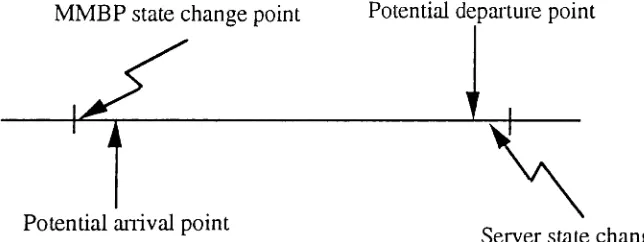
It is further assumed that arrivals can only occur at the beginning of each slot, and

that departing packets leave the system at the end of each slot. The state of the MMBP

changes only at the beginning of a slot just before arrivals occur, and the state of the server

changes only at the end of a slot immediately after the potential departure time (see Figure

2). For simplicity, we assume that the MMBP-stream packet has priority over the Bernoulli Process packet in the sense that the stream packet is served first if an

MMBP-stream packet and a Bernoulli Process packet arrive in the same slot.

In order to obtain the steady state queue length distribution, we observe the system

at the slot boundaries and generate the imbedded Markov chain [12]. In this Markov chain,

there are2(K+2)(N+ 1) states denoted by (V,S,I1) representing that the state of the MMBP is

represent the buffer size, and thus at most(K+1) packets are allowed in the system. There

are only three events that can cause the Markov chain to change state: the MMBP state

change, a packet arrival or a server state change. By solving the Global Balance Equations

of the Markov chain, the queue length distribution of the MMBP+BP/D(N)/l/K queue is

obtained.

3.

The

Queue Length Distribution Observed

at the Arrival

Instances of lVIMBP-stream Packets

In this section, we obtain the queue length distribution observed by the arrivals

from the MMBP-stream.This analysis will enable us to delive the waiting time distribution,

the blocking probability, and the interdeparture time distribution for the MMBP-stream

packets. The derivation of the interdeparture time distribution is given in detail in the

following section.

The system state as defined above is represented by three parameters, the MMBP

state, the state of the server, and the queue length. We observe the system state at arrival

instances of packets from the MMBP-stream, and relate the distribution of the system state

at the (11+ l)st observation point (the arrival instance of (11+ l)st MMBP-stream packet) to

that of the previous observation point, i.e., the nth observation point [2], [3].

We define a random variable

Ci

n) to represent the system state observed

immediately before the potential arrival point in kthslot following the nth MMBP-stream

packet arrival given that the (n+l)st MMBP-stream packet arrival does not occur in the

precedingk-l slots. ct) is a 3-tuple variable, ctJ=(Vin).s~n),Nt»),where Nt) and

st

l

represent the queue length and the server state respectively observed immediately before the

potential arrival point in the kth slot following the nth anival of a packet from the

MMBP-stream, and

vt

J_{indicates the MMBP state in which the nth MMBP-stream packet arrival}

seen by the nth MMBP-stream packet arrival. That is, V~"), N6") and S6") are the MMBP

state,the queue length and the server state accordingly seen by the nth arrival of a packet

from the MMBP-strcam. The main objective in this section is to determine the probability distribution of Cci")

For this purpose, we further introduce supplemental random variables. N~n) and

sin)

represent the queue length and the server state respectively observed immediately after

the potential arrival point at the kth slot following the 11th arrival of a packet Irorn the MMBP-stream.

Vi

n

) indicates the MMBP state in which the nth MMBP-stream packet

arrival occurred.

c»

is a 3-tuple variable

cr

=(\I(n)SIn) N(n») The order of

k ' k k ' k ' k •

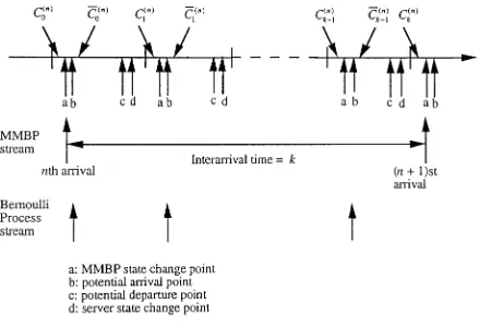
occurrence of the random variable observation points inaslot is presented in Figure3. Immediately afteran MMBP-stream packetarrival, there are

»:

+ 1+B packets in

the system, where B is a random variable representing the number of arrivals [rOITI the Bernoulli Process stream. Hence, we have the relation

N~n)

=

min(N6")

+

1

+

B, K

+

1), where B

=

{I

o

witli prob.

f3

witli prob. 1-

f3

(1)

Next, we consider the relation between N~n) and N_t( II ) . There are only three events

h b . . f N(1I) d N(1I)· ack td tur a

that can happen between t e two0 servauon points a . 0 an 1 · a pac e epar ure,

server state change, and the MMBP state change as shown in Figure 3. A departure occurs in a slot if and only if the state of the server before the potential server state change point is equal to

N

in the given slot. Therefore, the relation is given

by

the equation

o

~

sci

n ) <N

56")

=

N

(2)

Bysimilar reasoning, we have the following recurrence equations for k

>

O.

o

~ S~:)l

<

N

S( n ) - N

kl

-(4)

By

examining the order or events in a slot in Figure

3,

the relations between

sin)

and

Sk

Cff) for k

~

()can simply be derived as follows

S(II)

=

Sen)

k k '

S

- ( fI )

+

1

k-l

Sen) -k

-o

0< S(fI) < N

k-l

S- ( fI ) - N N(n) 0 or

k-l - , k-l >

S(fI) = N N(n)

=

0 or

k-I ' k - l

SUI)

=

o

N(ff) >

a

k-l ' k - l

Sen) = 0 N(n)

=

0

k-l ' k - l

(5)

(6)

Next, we consider the probability density ofthe random variables. Let c~n)(v,i,j)

and Ck(II)(v,i,}) be the probability density functions ofthe random variables cin) and ck(n)

• 0 I 0 c(n)( 0 0)-po b[V(n)- S(fI) - 0N(n) - 0] d c(n)( 0 0) P b

respective y, l.e., k V,l,J - 10 k -v, k - 1, k - J an k V,l,J

=

ro

[ y en)=V sCn)

=

i N(n)= JO]

k ' k ' k: •

Considering the relationship between therandom variables as given by (1) - (6), we

have

c~n)(v,i,j -1)(1-fJ)

+

Cci")(v,i,j - 2)fJ

Co(n)(v,i,}) = C~fI)(v,i,K)+ Ccin)(v,i,K-1)f3 + Ccin)(v,i,K

+

1)

o

v

=

0 or 1, 0::; i ~ N,

a

~

}

~(K

+

1),

O~j5:K

j = K+l

i>

K +1

(7)

Cifl)(v,i,})(l-

fJ)

+

Ci")(v,i,j-1)f3

ck(n)(v,i,j)=

Ci

n)(v,i,K ){3

+

C1n)(v,i,K

+

1)

o

O~j<5.K

}=K+l ,

i

>K+l

C( n ) ( • • )

k V,l,}

=

Ck(~~(V,O,O)

+

_Ck(~~(v,N,I)

C<1I)(

0

0) C(1I)( N· 1

k-l v, ,}

+

k-l v, -l

+ )

Ck-l<1I )('V,l -. 1·)«]

o

i

=

O,j

=

0

i=l,j>O

1<i~ N,j > 0

i= O,j >0 or 1~ i 5:N,j = 0

k ~ 1, v

=

0 or1, 0 5:i ~ N,

a

~ j ~ (K

+

1).

(9)

When a new packet from the MMBP-stream arrives in thekthslot following the last

arrival, the new packet finds the queue length

Ni

n

) and the state of the server s~n) upon its

arrival. Thus, the distribution of the system state seen by the(11+l)st MMBP-stream packet arrival, by using the distribution of the system state in the kth slot following the nth MMBP-stream packet and the probabilitydistribution that the(11+J)stMMBP-stream packet arrival occurs in thekth slot, can be obtained.

Since the MMBP is not a renewal process but aMarkov renewal process, the distribution of the time interval from nth arrival to (n+l)st arrival is not exponentially distributed but depends on the MMBP state at the time of the nth arrival. Therefore, we must use the conditional interarrival time distribution ay(v',k) (Probjinterarrival time = k

slots, state of the MMBP

=

v'Istate of the MMBP for the previous arrival v]), instead of a(k) (Prob[interarrival time

=

k slots]). A derivation of Qv(v',k) for a 2-state MMBP is given in Appendix. The probability density Ccin+l)(v,i,j) can be written as a function of

Cin)(v,i,}) as follows

OC)

C(n+l )( , ° 0) - " ( ' k)C<1I)( ..)

o V,l,} - L..Jov v, k V,I,}.

k=l

(10)

The steady-state probability that there arej packets in the queue, the state of MMBP is v, and the state of the server is

i

upon a packetarrival from the MMBP-stream is given

by

Co(V,l,j. 0)

=

1·irnC(1l)(0 v.i.] ,0.)

n~oo

Using Co(v,i,j) , the joint probability density of the MMBP state, the queue length

and the server state observed by a packet arrival from the MMBP-stream, the probability

density of the queue length observed at the arrival instances of MMBP-stream packets can

be simply obtained as follows

1 N

Prob[queue length

=

jla packet arrivalfrom MMBP streant]

=

IICo(v,i,j). (12)

v=O ;=0

The waiting time distribution and the blocking probability for the MMBP-stream

packets are also readily obtained using Co(v,i,j) .The waiting time for an MMBP-stream

packet is the time to serve all the packets found in the queue and in the server upon the

arrival of the given MMBP-stream packet. Since we assume that the MMBP-stream packet

has priority over the Bernoulli Process stream packet when an MMBP-stream packet and a

Bernoulli Process stream packet arrive at the same slot, the waiting time of the

MMBP-stream packet is not affected by the possible arrival from Bernoulli Process MMBP-stream in the

same slot. Given that the state of the server was

i

(>0) and that the num ber of packets in the

system wasj upon the given MMBP-streaITI packet arrival, the packet in the server requires

N -

i

+

1 time slots before its departure and the packets in the queue require (j -1)x N

time slots to be served. Thus the total waiting time is (N - i

+

1)

+

(j-1)x N slots, given that the MMBP arrival sees that the server state was i(>0) and the queue length wasj upon

its arrival. Thus, the probability density of the waiting time for the MMBP-stream packet is

given as a function of Co(v,i,}) as follows

d(k)=

1 N K+l

LLLCo(v,i,j)b(k,j

XN -,+1),

v=O;=1 j=1

k>O

k=O

(13)

The blocking probability for the strealTI is the probability that an

MMBP-1 N

stream arrival sees(K+1) packets in the queue. and is given by

L L

Co

tv.i,K

+

1) .

v=O ;=1

4. The Interdeparture Time Distribution for

the MMBP-stream

Packets

In this section, we derive the intcrdcparturc time distribution for packets from the MMBP-stream by using Co(v,i,j), the probability density of the system state observed at

the arrival instances of the MMBP-strealTI packets, obtained in the previous section.

For this purpose, we define the two-tuple random variables, Ci~;,q=(Nk,s,q' Sk,S,q)

and

C/:~q=(Nk.s.q.

Sk'S,q). Nk,s,q' and Sk,s,q represent the queue length and the server state

accordingly observed immediately before the potential arrival point at the kth slot following

an arrival of a packet from the MMBP-stream, and Nk .s.q , and Sk,s,q represent the queue

length and the server state respectively observed immediately after the potential anival point

at the A.1h slot following an arrival of a packet from the MMBP-stream, given that the state

of the server was s and the queue length wasq upon the arrival of the given MMBP-stream

packet, and the next MMBP-stream packet arrival does not occur inthe precedingk-I slots. By an argument similar to the one used in deriving (1) - (6), the relationships

between the above defined random variables are as follows

Nl,s,q = min(q

+

1

+

B, K

+

I), (14)

{ Nk .S .q

Nk,s,q

=

N -1

k.s.q

k ~ 1,

o

~Sk-l,s,q <N

Sk-l,s,q = N

Nk .s .q

=

min(q

+

B, K

+

1),

k> 1, (16)

Sk'S,q

+

1

Sk,s,q

=

1

o

k ~1.

0<Sk,s,q <N

s.:

=

N ,Nk.s .q >0 or Sk,,'\,q

=

O,Nk.s .q >0 Sk,s,q =N,N_{t .}s .q =0

or

Sk'S,q =O,N_{k .}s .q =0

(17)

The corresponding joint probability densities are denoted as Ck,s,q(i,}) =

Prob [Sk.s.q

=

i.Nk.s.q

=

j] and Ck,s.qU,j)

=

Prob [Sk'S,q

=

_i,Nk.s.q

=

j] and are determined

through the following equations.

f3

Cl,s,O

o.»

= 1-

f3

a

o

~

s.i

~ N, 0~ j ~ (K

+

1),

C

o.» -

I

PI-

f3

l.s.q I,)

-l

0

s

=

O,}

=

2,i =

°

s = O,}

=

l,i

=

°

otherwise

S,*O,}=q+2,i=s

s,*O,j=q+l,i=s

otherwise

(18)

o

~

s.i

s

N, 0

<

q

<

K, 0

s }

~ (K

+

1), (19)

_

{I

C1.s.q(i,j)= 0

s ;t:.

O,i

=

s.]

=

K

+

1

otherwise

o

5:

s.i

~ N,

q

=

K,K

+

1, 0~ j ~(K

+

1),

Ck-1,s,q(i,j)(l -

(3)

+

Ck-l,s,q(i,j-1)f3

Ck,s.q(i,j)= Ck_l.s,/i,K)P

+

Ck-l.s.qU,K

+

1)

o

O~j~K

j=

K+l

i>

K+l

k

>

1,

0

~

s.i

s

N,

°

~ q,j ~ (K

+

1),

Ck,s,q(O,O)

+

C_k,s,q( N , l )

C Ck,S.q(O.j)

+

Ck.s,q(N.j

+

1)

k.s.q(i,j) =

C_{k •}s•q(i - 1,j)

°

k~l, O~s,i~N, 0<_{- q,J -}o«K+1)_.

i = O,j =

°

i= l,j >0

1<

i

~ N,j >0

i

= O,j >

°

or 1~ i ~ N,j =

°

(21)

(22)

Now, we consider the interdeparture time between two MMBP-stream packets. The

system time of a packetfrom the MMBP-st.ream is defined as the length of the time interval

starting from the slot when the arrival of the given packet occurs and ending at the slot

when the given packet departs the system. Let l-v(s,q) denote the system time of a packet

from the MMBP-stream given that the queue length was q and the server state was supon

its anival. Then

{

(q-l)N

+

(N - S

+

1)

+

N

~v(s,q) =

N+l

q>O

q=O

(23)

Using ~v(s,q),the random variable

IDk,S,q

denoting the interdeparture time between

two consecutively arriving packets from the MMBP-stream when the interarrival time

between two packets is k, and the server state and the queue length upon the arrival of the

first packet of the two are sand q respectively, is given by

(24)

From (23) and (24), idk,s,q(j) , the probability density of the randorn variable

ID

_k ' is obtained as

.s.q

idk.s,q

(j)

=

N

{C,.

(i,(j - k

+

i

+

qN -

s) /

N)}

L

~.s,q .

;=1

+C

_k'S,q(O,O)8 (J,k - qN + s)

N

{C

_k (i,(j-k+i)/ N)}

L

.s.q

;=1

+C

_{k •o.o}(O,O)8(j ,k )

q>O

q=o

Finally, we remove the conditions from the above equations to obtain the probability density of the interdeparture time for the MMBP-strealn as follows

00 N K+l 1

id(j) = LLLLa.,(k)Co(v,s,q)idk.s.q(j),

k=l s=O q=O v=o

1

av(k)

=

Lav(v',k). v'=o

(26)

5. The

Autocorrelation

of the

Interdeparture

Time

for

the

lVllVIBP-stream Packets

In this section, the autocorrelation coefficient of the interdeparture time for the MMBP-stream packets is derived [7]. We define two random variables:Tn' the interdeparture time between the (n-l)st and the nth packets; Tn,(v,s,q)' the interdeparture time

between the (n-l)st and the nth packets given that the state of the system upon the nth

packetarrival [rom the MMBP-stream is (v,s,q).

The autocorrelation coefficient of the interdeparture time of the MMBP-stream with lag 1is given by

Cov(T,,_1Tn) _{E(Tn_1}Tn) - E(T_{n_1})E(T_n)

qJt = Var(T,,) = £(T;) - £2(T,,) . ₍₂₇₎

We can easily determine _{E(Tn)(=E(Tn_}I» by using the probability density of the

interdeparture time distribution for the MMBP-stream derived in the previous section. To obtain the term _{E(Tn_1}Tn)' we again introduce a number of z-transforms. Let

T . . ( I )

A , .. (z) == E[z n.(v·,s.q >IC

on-

=

(v,s,q)],

(V,s,q)(v .s ,q )

(z) - E[.-rTnIC(,,-I) - ( )]

B(v,S,q) c

=

~ 0 - v,s,q ,

d C ( ) - E[.-rT"-1 r,Ic(n-l) - (' q)]

To derive A(_{v.s ,q})('._{v .s ,q},)(z), we define t(_{v,s,q)( v}, ' ._{.s ,q )} as the time interval beginning from a

particular slotat which a packet, whose arrival occurredwhen the state of the system was

(v,s,q), from the MMBP-streUlTI departs and ending at a slot when the next MMBP-stream

packet, upon whose arrival the state of the system was (v',s',ql), departure occurs.

t( ..S )(v' , ,)=jwith probability jJ(, ' . ,)(j)

=

prob[interdeparture time of thenth andthe

. " q .s ,q ~,s,q)(v.s .q

(n+1)st MMBP-stream packets =

j,

state of the system upon the arrival of the (n+l)st

MMBP-stream packet= (v',s',q') Istate of the system upon the arrival of the nth

MMBP-stream packet

=

(v,s,q)]. Therefore,

ee

A_{(~'.s,q)(\.·',s.q)}. . (z)='p_{£..J (v,s,q)(\.".s ,q)}.. (J')7j

" v .

j=l

(29)

p , , . (j) can be obtained by using the conditional interarrival time distribution

(v,s,q)(v .s ,q )

a,

(v',k) and the probability distribution of the system state observed at the arrival instances

of the MMBP-stream packets Co(v,s,q)

C1('t

p .. , (j)

= "

a_v(v' ,k )C_o(v,s,q )8 ( j , {k

+

w(s'

.q) -

l-v(s,q)}).

( v.s ,q )(v,s ,q ) £..J

k=l

By using (28), we obtain

1 N K+I

B(v.s.qj(z) = L L LA(v.s.q)(V,.s',q'j(z), (30)

~"=Os'=Oq'=O

I N K+l

C(V,s.qj(Z"Z2)= L L LA(v,s.q)(v',s·.q)Zt)B(v·.s"q,/z2)' (31)

v'=Os'=Oq'=O

Further, we denote the matrix of A , , . (z). the vector of B(v,s,q)(z), and the vector of (V,s,q)(v .s .q )

C(V.S,qj(ZI'Z2) byA(z) ,B(z), and C(ZI'Z2) respectively. Equation (31) is then rewritten in

matrix form as follows

(32)

where

Co

is the probability vector of the probability density Co(v,s,q).

Finally, we can readily derive E(T T) Irorn E(zT fI_, _TfI ) as ,,-1 " 1 ~2

E(T T) = C dA(Zt) dB(Z2)

"-1,, 0 d:

1-~l (~2 z,=1.':2=1

,and the autocorrelation coefficient of the interdeparture time for the MMBP-stream is

obtained by substituting _{E(Tn_1}Tn) in equation (27).

6. Numerical Results

In this section, numerical examples are presented by employing the analytical

approach presented above. For the numerical computation to be tractable, we approximate

the interarrival time and the interdeparture time distribution between packets such that the

maximum time is finite. We will investigate how the traffic characteristics of the

MMBP-stream are influenced by the amount of BP-MMBP-stream traffic, the degree of the burstiness and

the correlation of the MMBP-stream.

The parameters assumed for the arrival process and the system are given in each figure. Lamda, CC, C2,

p,

K, and N represent the average probability of an arrival for the

MMBP-stream, the autocorrelation coefficient of the MMBP-stream, the C2 value of the

MMBP-stream, the arrival rate of the BP-stream, the buffer capacity of the system, and the

deterministic service time respectively.

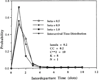
Figures 4 and 5 show how the probability densities of the interdeparture times of

the MMBP-stream change as the BP-stream traffic increases. For comparison purpose, we

also include the probability density for the interarrival time distributions of the

· In Figure 4, we observe that the probability densities are less peeked as the arrival

rate of the BP-stream increases (~

=

0.1, 0.3, 0.5). That is, the probability of

interdeparture time equal to 1 gets smaller and that of the interdeparture time equal to 2 gets

larger as the amount of the Bf'<strcam increases. This is because the packets from the

BP-stream tend to interleave the continuously arriving packets from the MMBP-BP-stream.

In Figure 5, however, we observe the opposite phenomina, i.e., the probability

densities of intcrdeparture time gets more peeked as the amount of the traffic from the

BP-stream increases (~

=

0.5, 0.9, 1.0). When

p

is equal to 1.0, the interdeparture time

probability density nearly overlaps the interarrival time probability density. As the value of

p

increases the buffer gets full more frecquently and large amount of BP-stream packets are

lost. This results in reducing the effect of the BP-stream to the performance of the

MMBP-stream, and thus the probability density of the interdcparture time becomes similar to the

original interarrival time distribution of the MMBP-streaITI.

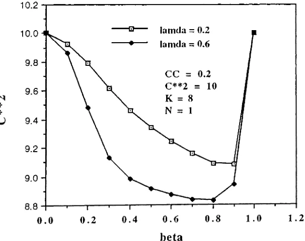
Next, we see the autocorrelation coefficient with lag 1 and the C2 of the interdeparture time of the MMBP-stream packets dependent on the amount of the traffic

from the BP-stream in Figures 6 and 7. We observe that the correlation of the interdeparture time becomes larger, and the C2of the interdeparture time gets smaller as the arrival rate of the BP-stream increases. The change is more rapid when

A

=

0.6 than when

A

= 0.2. However, the correlation starts to decrease and the C2 starts to increase as the

arrival rate of the BP-stream increases to exceed a certain limit due to the BP-stream packet

loss as explained above. When A

=

().6, the value of this limit is smaller. In the extreme

case, when

~

= 1.0, the correlation and the C2of the departure process approach to those

of the arrival process of the MMBP-strealTI.

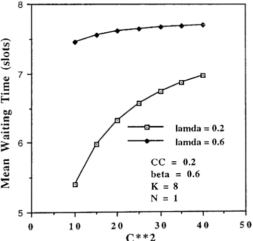
Figures 8 shows the mean waiting time for a packet from the MMBP-stream as a

function of the amount of traffic from the BP-stream. Since the deterministic service time is

1nus, tne waiting time of an MMBP-stream packet when ~ is 1.0 is equal to the buffer

capacity, K=8. We observe that the mean waiting time when A

=

0.6 grows more rapidly

than that of

A

= 0.2 as

P

increases from 0.3 to 0.4, see in Figure 8. This is because the

buffer is filled up faster when the total load of the system is larger, that is, when

A

is

larger: Since we have a finite capacity system, the amount of mean waiting time increase is

reduced as the total load increases to exceed a certain limit due to packet loss.

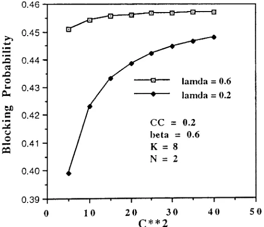
Figure 9 shows the blocking probability for the MMBP-stream packets. Similar to

the mean waiting time, the blocking probability increases rapidly as ~ increases, and as the

load of the system exceeds a certain limit the amount of increase is reduced.

The mean waiting time and the probability of blocking for the MMBP-stream

packets dependent on the correlation and the burstiness of the MMBP-stream are shown in

Figures 10 - 13. The mean waiting time and the blocking probability for the MMBP-stream

increases in a logarithmic fashion with increase in burstiness and show an exponential type

increasewith increase in autocorrelation.

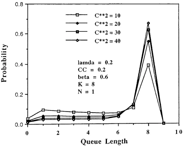
Figures 14 and 15 show the queue length distribution at arbitrary points in time.

Figures 16 and 17 show the queue length distribution at MMBP-stream packet arrival

instances dependent on the autocorrelation and the burstiness of the MMBP-strealn. We

observe that the queue length distributions at arbitrary point in time are less sensitive to the

changes of MMBP-stream characteristics.

7. Conclusion

In this paper, we studied a queueing model which is particularly motivated by the

study of the link-transport layer servicing several transport connections including an XTP

connection in a high speed network. We have analyzed a discrete time finite capacity

arrival processes, two kinds of traffic streams, MMBP and Bernoulli Process, are considered.

The queue length distribution of MMBP+BP/D(N)/1/K queue at arbitrary points in time using a multi-dimensional Markov chain analysis is obtained first. The queue length distribution observed at the MMB P-stream packet arrival instances, and the waiting time distribution and the blocking probability for the MMBP-stream are then obtained to investigate how the MMBP-strealTI is affected in the queue. The probability density and the

autocorrelation coefficient of the interdeparture time distribution [or the MMBP-streaITI, which are important in the analysis of network of queues, are also derived.

The numerical examples show that the traffic characteristics and the performance for the designated transport connection are affected by the external traffic load, the degree of burstiness and correlation of the traffic source.

References

[1] W. Stallings,Data and Computer Communications, Macmillan Publishing Company, Macmillan, Inc., NJ, pp134-147, 1991.

[2] H.Heffes and D. M. Lucantoni, "A Markov modulated characteristics of packetized voice and data traffic and related multiplexer performance," IEEEJ.on Select. Areas

C0I11111Lll1., vol. SAC-4, no.

6,

pp. 856-868, Sept. 1986.

[3] Masayuki Murata, Yuji Oie, and Tatsuya Suda, "Analysis of a Discrete-Time Single-server Queue with Bursty Inputs for Traffic Controlin ATM Networks," IEEEJ.011

Select. Areas C0I11111UI1., vol. 8, no. 3, April 1990.

[4]

Yoshihiro Ohba, Masayuki Murata, and Hideo Miyahara, "Analysis of Interdeparture

Processes for bursty Traffic in ATM Networks," IEEE J. 011 Select. Areas

Co111111ll11. , vol. 9, no. 3, April 1991.

[6]

~rne

A. Nilsson and Meejeong Lee, "A Performance Study of the XTP Error Control," Proc. 4th IFIP conference on High Performance Networking, Liege, 1992.

[7] W. Fischer and K. Meier-Hellstem, "The MMPP Cookbook," draft, Oct. 1990.

[8] U. Briem, T. H. Theimer and H. Kroner, "A General Discrete-Time Queueing Model: Analysis and Applications," TELETRAFFIC AND DATATRAFFIC in a

period of Cliange, ITC-13, Elsevier Science Publishers B.V. (North-Holland) lAC,

1991.

[9] J.R. Louvion, P. Boyer, and A. Gravey, "A Discrete-Time Single Server Queue with

Bernoulli Arrivals and Constant Service Time," Proc. 12th International Teletraffic

Congress, Torino, 1988.

[10] I.Jacobs, "Design considerations for long-haul lightwave systems," IEEEJ. Select. Areas CO/1l1J1UI1., vol. SAC-4, pp. 1389-1395.

[11] Dooyeong Park, Henry G. Perras, and Hideaki Yamashita, "Approximate Analysis

of Discrete-time Tandem Queueing Networks with Bursty and Correlated Input

Traffic and Customer Loss," Technical Report, Department of Computer Science,

NOlth Carolina State University, Raleigh, NC, 1992.

[12] L. Kleinrock, Queueing System, Vol. I, John Wiley & Sons, Inc., New York, NY,

Appendix

A two state MMBP is characterized by the transition probability matrix Ptand the

arrival rate matrixA defined as the following:

P

t

=

[p

1-

P]

l-q q and

Lett_vv'be the time interval starting [rom a particular slot when the arrival process is

instate vand ending at a slot when the nextarrivaloccurs and thearrival process is in state

v'. Then,

1

tIl

=

1

+

tIl

1

+

t₂₁

1

f_{I 1}= 1

+

tI 2

1

+

t22 1 tIl

=

1

+

t12

1

+

t22

w.p. alJ

l-v.p. (1- a)p

rV.p. (1 - (3)(I- p),

w.p.

a(l- q)

w.p.

(l-a)(l-q)

w.p.

(1-f3)q,

w.p. (3(1-p) l-v.p. (1- a)p

w.p. (1- (3)(1- p),

w.p.

f3q

w.p. (l-a)(l-q)

w.p. (1- [3)(1- q).

Define

Sn

as the state of the arrival process when the nth arrival occurs, and Tn,v as

the interarrival time between the (n-l)stand nth arrivals while the nth arrival occurs in state

v. If we define

Avv' == E[,.,Tn,v'ISc, ,,-1 = v]'

then from the definition oftvv' and Tn, v we have

A

=

E[,.,/

w_{' ]}

Therefore,

All(Z)

=

apZ

+

(1-a)jJzA_1I(z)

+

(1- ,8)(1-P)~l(z),

~1(z)

=

a(l-q)z

+

(1-a)(I- q)zA_{I I}(z)

+

(1-{3)q~1(z),

Al 2(z) =f3(1- p)z

+

(1- a)PzAl 2(z)

+

(1- [3)(1-p)~2(z),

~2(z)

=

f3qz

+

(1-a)(I-q)zAl 2(z)

+

(1-{3)q~2(z),

By

solving (33) - (36) we can obtain Ayy'(z) with respect to0,

b,

jJ, q as follows

A (~)= ajJz + z2a (1 - {3 )( 1- p - q )

11 c 1 n 2 '

-z(p(l-a)+q(l-fJ»-z (1-a)(1-{3)(I-p-q)

~l(Z)=

a(1-;)z ,

1-z(p(l-a)

+

q(1- f3» - z (1- a)(l- (3)(1-p - q)

A (-) = f3(1- p)z

12 c l-z(p(1-a)+q(1-,8»-z2(1-a)(1-{3)(1-p-q)'

A ( ) _ ,8qz

+

Z2,8(1-a)(I- p - q)

22 Z - 2 •

1- z(p(1- a)

+

q(l-

(3» -

z

(1-a(l- f3)(1- p - q)

(33)

(34)

(35)

(36)

(37)

(38)

(39)

(40)

The conditional probability density function of the interarrival time, Qv(v',k),can be

obatined by inverting the generating function, Avv'(z). Let C~,y'(k) and

b;

(k) be the

coefficient of the zk in the numerator and the denominator ofAvv'<z) respectively. Then we

have

2

"£..Jcy V '(k)zk 00

A I(~)

=

k=O

=

'a

(VI k)~k

vv ~ 2 £..J v ' ~

Lb,.y. (k)/ k=O

k=O

For each equation, multiplying both sides by the denominator and the equating the

coefficients ofzkon both sides, we obtain the following set of linear difference equations

min{2.k) {Cvv.(k) k = 0,1,2

L ay(v',k-n)bvv·(n)=

a

k>2

n=O

We can then solve forQv(v',k) recursively as follows

1 [ m i n ( 2 , k ) ]

ay(v' ,k)

=

C_{vv' (k) -} Lbvv' (n)ay(v'.k-n) ,

b;

(0) n=l

where cy V'(k)=

0

for k

>

2.

p

I - P

1 - q

Figure 1: The Markov chain of a two-stale MMBP

q

MMBPstate change point

Potential arrival point

Potential departure point

Server state change point

nth arrival

ab

c(n)

o

MMBP stream

Bernoulli Process

stream

t

c d ab

t

c

d

Interarrival time= k

c(n)

k-l

c(n) c(n)

k-l k

a b c d ab

~t

V1

+

l)st arrival

t

a:MMBP state change point b: potential anival point

c:potential departure point d: server state change point

0 . 8 . - - - _

12 10 8 6 4

lamda = 0.2 CC = 0.2

C**2 = 10

K=8

N = 1

- a - beta

=

0.1

• IJeta

=

0.3

a beta=0.5

o Interarrival Time Distrihution

2

0.0 . .--r-~-....;....:::::~!!!CI...

-a--a--...

--IJ----l

o

0.6 ~ ...

....

-....

~ ~ _0.4 ~ 0 ~ c, 0.2

Interdeparture Time (slots)

Figure 4: Interdeparture time distribution [or the MMBP-stream w.r.t. the amount of the

BP stream (~ = 0.1, 0.3, 0.5).

0.8

-r---0.6

~ _beta

=

_0.5

•

beta

=

0.9

~

•

beta = 1.0

...

....

_0.4 0 Interarrival Time Distributlon

-....

~

~

~

0 _lamda

=

_0.2

~

Q.. _{CC = 0.2}

0.2 _{C**2 = 10}

K=8

N = 1

0.0

0 2 4 6 8 10 12

In terdeparture Time (slots)

Figure 5: Interdeparture time disttribution for the MMBP-stream w.r.t. the amount of the

0.22 ,

-§

0.21 .~

...

~ Qj s... s... o ~ o :; 0.20

<

--e-- lamda=0.2

• lamda

=

0.6

CC

=

0.2

C**2 = 10

K

=

8 N = 1

1.2 1.0 0.8 0.6 beta 0.4 0.2 O.19-r--,r--~-~___,.-_r____,r____r_-...,...____,.-...,.____..-_I 0.0

Figure 6: Autocorrelation of the interdeparture time distribution [or the MMBP-stream as a function of the amount of the BP stream.

1.2 1.0

0.8

CC

=

0.2

C**2 = 10

K=8

N

=

1

~ lamda=0.2

• larnda=0.6

0.4 0.2 10.2 10.0 9.8 9.6 N

*

*

U 9.4 9.2 9.0 8.8 0.0 0.6 beta

Figure 8: Mean waiting time [or the MMBP-stream packets as a function of the amount of

the BPstream packets.

0.5

~

~

.-

~ _0.4

.-

~

~

~

0

~

Q..

0.3 eo

c:

.-

_~

~

0

~

~ 0.2

~ lamda=0.2

• lamda=0.6

CC = 0.2

C**2 = 10

K=8 N=2

1.0 0.8

0.2

O. 1-+-_ _- __-...--~-~-r_____,r___,.-__,_-_t

0.0 0.4 0.6

beta

Figure9: Blocking probability for the MMBP-stream packets as a functionof the amount of

7 ....- - - . . . ..-... til

...

0 fii ' - ' Q) ₆

e

~ ell C .,..

...

.

;

~ 5

=

~ QJ ~

lamda

=

0.2 C**2

=

10 beta

=

0.6

K=8 N

=

1

0.5 0.4

0.2 0.3

CC

0.1

4 - t - - - - , r - - - - . . . . - . . . - - - . . . - - . . . - - - -...

0.0

Figure 10: Mean waiting time for the MMBP-stream packets as a function of the degree of

the correlation of the MMBP-stream.

50

40

•

•

CC

=

0.2 beta

=

0.6

K=8 N

=

1

~ lamda=0.2

• lamda

=

0.6

•

10 8 ,..-... til ... 0 Vi ' - ' QJ 7

e

~ eo c .,.. ...

.

;

~ 6 C ~ QJ

....

e.

5

0 20 30

C**2

Figure 11: Mean waiting time for the MMBP-stream packets as a function of the degree of

0 . 4 . -0.5 0.4 0.2 0.3

CC

0.1

lamda = 0.1

C**2 = 10 beta = 0.3

K=8

N = 2

o.1-t----,r----r'-.,.----r-~__,..___...,..-...____..-~

0.0 >, ~

...

-:.c

~ 0.3 ,.Q o ~ Q.. eo

c:

:g ~ 0.2 o

-~

Figure 12: Blocking probability for the MMBP-stream packets as a function of the degree of the correlation of the MMBP-stream.

50

40

CC

=

0.2

beta = 0.6

K=8

N

=

2

- - e - - lamda =0.6

• lamda

=

0.2

10 0.46 >a 0.45 ~

...

-...

0.44 .Q ~ ,.Q 0 s. _0.43 Q.. eo c 0.42

:;;

u 0 0.41

-

CQ 0.40 0.39

0 20 30

C**2

10 8 2 0.0 -t----r---r---....,---r---.,..--...---~----.I

o

0.8

- a - _{CC = 0.001}

•

CC = 0.1

0.6 a CC = 0.2

~ 0 _{CC = 0.3}

~

.~

--

•

CC = 0.4

.~

~

~

"Q _{0.4 lamda = 0.2}

0

I-l C**2 = 10

0.- _beta

0.6

= K=8

0.2 N = 1

4 6

Queue Length

Figure 16: Queue length distribution at the MMBP-stream packet arrival instances w.r.t. the

degree of the correlation of the MMBP-stream.

10

8

4 6

Queue Length

2

O.a- ¥ - - _ _- _ - . . . - - . . r - - - , . - - - , . - - - - r - - - D - - - i

o

0.8

~ _{C**2 = 10}

•

C**2=20

0.6 a C**2 = 30

0 _{C**2 = 40}

~

..-.-

-

.~

"Q

lamda 0.2

~ _0.4 =

..c _{CC = 0.2}

0

I-l _{beta = 0.6}

Q.

K=8

0.2 N = 1

Figure 17: Queue length distribution at the MMBP-stream packet arrival instances w.r.t. the