A Case Study and Analysis of Cleanroom Energy Use

(1)

ABSTRACT

SIMON, MICHAEL JAMES. A Case Study and Analysis of Cleanroom Energy Use. (Under the direction of Dr. Stephen Terry and Dr. Herbert Eckerlin).

A plant has a cleanroom HVAC system which is known to be a large energy user. This study found that the current cleanroom operation is indeed wasteful, and stands to benefit from improved controls and operation protocols. Proper data collection is instrumental in understanding how the system is operating. After analyzing data, the real cleanroom operation was found to be different than the assumed cleanroom operation, a significant conclusion.

Data on cleanroom conditions, power draw for both dedicated cleanroom chillers, and power use of all five air handling units are collected. It is revealed that cleanroom chiller and reheat power cost is approximately $103,000/yr, much higher than necessary, but also much less than the original estimate of $385,000/yr. During the data collection process, changes to the cleanroom operation were made, and some of them are seen to have desirable results, but there are also very negative unintended consequences, which are seen in the data collected. The cleanroom reheats are now seen to be sensitive to times of high humidity, using an average of 200 kW of electric strip reheat when the dew point is above 50°F.

(2)

thought is unknown. The data collected from this project forces the plant to take a second look into how completeness and accuracy of its control setup.

(3)

A Case Study and Analysis of Cleanroom Energy Use

by

Michael James Simon

A thesis submitted to the Graduate Faculty of North Carolina State University

in partial fulfillment of the requirements for the degree of

Master of Science

Mechanical Engineering

Raleigh, North Carolina May 8, 2009

APPROVED BY:

_______________________________ ______________________________

Dr. Stephen Terry Dr. Herbert Eckerlin

Committee Co-Chair Committee Co-Chair

(4)

ii

DEDICATION

(5)

iii

BIOGRAPHY

Michael Simon was born at Touro Infirmary in New Orleans, Louisiana on August 7th, 1984. His parents soon moved to Greensboro, North Carolina, and, as a 5 year old, he had no

choice in the matter. Greensboro was kind to young Michael, and he graduated with honors from Walter Hines Page High School in 2003. Heading to North Carolina State University to study Engineering, he was soon attracted to Mechanical Engineering, where he took a

(6)

iv

LIST OF TABLES

Table 1.1: Energy Cost from Rate Schedule ... 2

Table 3.1: Logger Locations and Descriptions ... 16

Table 4.1: Chiller Power Totals ... 64

Table 5.1: July Chiller Power Cost ... 78

Table 5.2: Extrapolated Chiller Energy Cost ... 79

(9)

vii

LIST OF FIGURES

Figure 1.1: Daily Real-time Pricing Unit Electric Rates at Summer & Winter Peaks [2] ... 3

Figure 1.2: Rough Plant Sketch ... 4

Figure 1.3: Outside and Plant Space Conditions ... 4

Figure 1.4: Cleanroom Zone Layout ... 5

Figure 1.5: Sample AHU Setup ... 9

Figure 1.6: Outside and Cleanroom Space Conditions ... 9

Figure 3.1: Diagram of AHU Data Recording ... 15

Figure 4.1: AHU 1 Typical Currents ... 20

Figure 4.2: AHU 1 Typical Power ... 22

Figure 4.3: Outside Dew Point Error ... 23

Figure 4.4: Cleanroom Chiller Temperature Collection Diagram ... 25

Figure 4.5: Chilled Water Temperatures and Chiller Power, June ... 26

Figure 4.6: Cleanroom Chilled Water Temperatures ... 27

Figure 4.7: Chilled Water Temperatures and Chiller Power, September ... 28

Figure 4.8: Chilled Water Temperatures and Chiller Power, Winter ... 29

Figure 4.9: AHU 4 Currents... 31

Figure 4.10: Cleanroom Supply Air Conditions ... 32

Figure 4.11: Cleanroom Temperatures and Dew Points, June... 35

Figure 4.12: Cleanroom Temperatures and AHU Power Usage... 36

Figure 4.13: Cleanroom Temperatures, Chiller Power, and AHU Power ... 37

Figure 4.14: Cleanroom Temp and AHU 3 & 4 Reheat ... 38

(10)

viii

Figure 4.16: AHU 1 Energy Setup ... 40

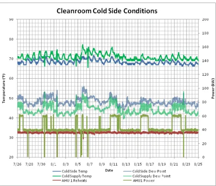
Figure 4.17: Cleanroom Cold Side Conditions, August ... 43

Figure 4.18: Hot Side Overview, Winter ... 44

Figure 4.19: AHU Typical Reheat Operation, Summer ... 46

Figure 4.20: AHU Typical Total Operation, Summer ... 47

Figure 4.21: AHU Typical Reheat Operation, Winter ... 48

Figure 4.22: AHU 4: Total Power and Reheat ... 49

Figure 4.23: Winter Cleanroom Operation ... 50

Figure 4.24: AHU Power, 9/22-9/29... 52

Figure 4.25: Outside and Plant Space Conditions, 9/22-9/29 ... 53

Figure 4.26: 9/22-9/29: Hot Side Data ... 54

Figure 4.27: AHU 2 Humidifier... 56

Figure 4.28: Chiller Power Consumption over Different Modes of Operation ... 60

Figure 4.29: Cleanroom Chilled Water Temperatures, August ... 62

Figure 4.30: Cleanroom Chiller Power, July ... 63

Figure 4.31: Cleanroom Chiller Power (Single Week) ... 65

Figure 4.32: Temperature and Dew Point with Chiller Power (One Week Graph) ... 66

Figure 4.33: Temperature and Dew Point with Chiller Power (Two Week Graph) ... 67

Figure 4.34: Chiller Power and AHU Power ... 68

Figure 4.35: Cleanroom Chiller Power (6/23-6/29) ... 69

Figure 4.36: Cleanroom Chiller Power (9/13-9/26) ... 71

Figure 4.37: Chiller Power and Outside Temperature, November ... 72

(11)

ix

Figure 5.1: Cleanroom Temp, AHU Power, and Cleanroom Chiller Use ... 74

Figure 5.2: Average Power vs. Average Outdoor Temperature ... 76

Figure 5.3: Average Power and Average Outdoor Temperature ... 77

Figure 6.1: New AHU 1 Winter Setup... 84

Figure 6.2: New AHU 1 Summer Setup ... 86

Figure 6.3: New AHU Operation with Outside Conditions ... 88

Figure 6.4: New AHU Reheat ... 89

Figure 6.5: Reheat Comparison ... 90

Figure 6.6: AHU and Chiller Operation with Outside Conditions ... 91

Figure 6.7: New Operation Hot Supply, Reheat, and Chiller Power ... 92

Figure 6.8: Cold Supply Temp and Reheat ... 94

Figure 6.9: Hot Side Conditions, Plant Temperatures and Reheat ... 97

Figure 6.10: AHU 2 and Outside Conditions ... 99

Figure A.1: Energy Balance on August 2nd ... 107

Figure A.2: Two Week Cleanroom Chiller Power, August ... 108

Figure A.3: Cleanroom Chiller Power, July 9-16 ... 109

Figure A.4: AHU 2 Current and Outside Conditions ... 110

(12)

1

Chapter 1: Introduction

The objective of this thesis is to provide a case study and analysis of the HVAC energy use of one particular cleanroom. This study stems from a North Carolina State University Industrial Assessment Center audit done at this facility, when it was estimated that the cleanroom uses 338 tons of cooling, and 750 kW of electric reheat, for a total cleanroom HVAC energy cost of about $385,000/yr. The reheat was thought to be needed because there is not enough of a heat load in the room, which is closely related to the problem of

overcooling. Doing some quick calculations led us to believe that the facility could save around $315,000/yr of this number, the vast majority of which is assumed to be reheat savings. This study was commissioned to measure cleanroom parameters, determine the current cleanroom operation, identify the savings possible, and suggest improvements on the current operation.

1.1 Cost of Energy

Because of confidentiality issues, specific details of plant operation, product, size, and location cannot be disclosed. Fortunately, for the purposes of this study, that information is largely irrelevant anyway.

(13)

2

The middle tier will be used in this analysis in order to not disclose plant size. Duke also differentiates between on-peak power at about $0.0453/kWh and off-peak power at about $0.0273/kWh. On peak during the summer is identified as the hours between 1 p.m. and 9 p.m. M-F, and during the winter as 6 a.m. to 1 p.m. M-F. All other times, and some various holidays are designated as off-peak. Also note that demand is only set during times that are designated as on-peak, although there is a nominal charge for excess off-peak demand, termed economy demand, as shown in the Table below.

Table 1.1: Energy Cost from Rate Schedule

June-September ($/kW)

October-May ($/kW) First 2,000 kW demand $10.9490 $6.4446 Next 3,000 kW demand $10.0296 $5.5167 Over 5,000 kW demand $9.1017 $4.5804

(Economy Demand) $0.8688 $0.8688

By including demand cost with on-peak power usage, one can quickly see that the cost of electricity on-peak is more than twice what it is off-peak. This is very difficult to quantify exactly, because just a single 30 minute interval of high power use will negate an entire month of demand reduction efforts. A good example of this is the extra cost in demand of that air conditioning system on a hot, muggy southern sunny summer day. Although this is clearly a regional rate, this is representative of how power companies bill on a national basis.

(14)

3

Figure 1.1: Daily Real-time Pricing Unit Electric Rates at Summer & Winter Peaks [2]

Figure 1.1 from Shan K. Wang [2] is dated by about 10 years, but it perfectly demonstrated why companies desperately want to avoid having to provide that extra kW. It hurts their profit margins.

1.2 Cleanroom Description

(15)

4

Figure 1.2: Rough Plant Sketch

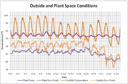
The facility itself is air conditioned, and this will be key in understanding the cleanroom operation. Below, in Figure 1.3, plant and outside conditions are shown on the same graph over a 15 day period. This graph is a summer month (June), and the relationship of outside temperature to plant temperature is there but severely mitigated, and the effect of dew point swings is mitigated as well, although to a lesser degree. This is important as it pertains to clean room infiltration, and heat gain or loss through the walls and roof.

Figure 1.3: Outside and Plant Space Conditions Plant Floor

(16)

5

The cleanroom as currently set up is not pressurized, although the plant is in the process of changing the current operating protocols and systems, which will be discussed in detail in Chapter 5 later in the report. The cleanroom operates 5 zones: Zones 1-4 are in the

cleanroom proper, and zone 5 is in the cleanroom entrance area. All of the zones are similar in size, but due to process changes since the cleanroom was constructed, zones 1, 3 and 5 serve areas with little heat load. Zone 5, however, does not have the precise temperature and humidity controls placed on it that zones 1-4 do, and it is served by a much smaller AHU and electric reheat.

Figure 1.4: Cleanroom Zone Layout

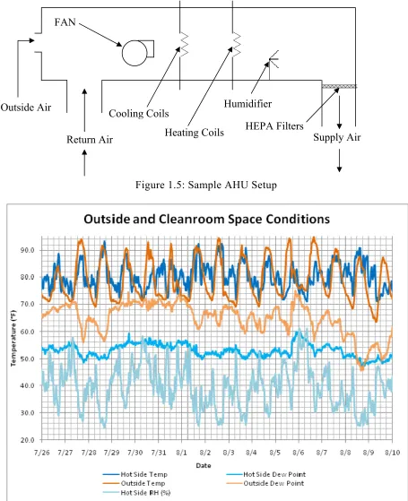
Zones 1-4 are served by AHU’s 1-4, each of which is a separate air handling unit. Notice the dashed lines in Figure 1.4. The AHU zones 1-4 are not separated in the cleanroom itself by any kind of wall or shield. So people, goods, and air can move freely between the 4 zones. Only zone 5 has a wall between it and zones 2 and 4, but even it has open doorways to zones 2 and 4. These AHU’s are provided cooling through two dedicated 240 ton air-cooled chillers, and reheat is provided by electric strips. Operating as a class 10,000 cleanroom (explained in Chapter 2), 180,000 cfm of air enters the return ducts goes through the fans. After this, it goes through the cooling coils, which cool the air to approximately 55°F, due to the control system. After going through the cooling coils, the air then goes through the reheat coils, and the air is brought back up to near room temperature, typically 65-70°F. Next, the air goes through the humidifiers, where air is humidified if necessary.

After this, it goes through the HEPA filters on the way back to the room. 3 4

(17)

6

This is how the cleanroom system was thought to operate before this project was started. Chapter 7 will present some postulated variations to the system as described above, and Chapter 6 will present the new operation, as conceived and after 2 months of data recording.

At the beginning of the study a total of 5,000 cfm of extra air was brought in from the outside as makeup air. This air is but a small trickle flow through each of the 4 main AHU’s. The cleanroom needs this makeup air because there is an exhaust flow of about 6,000 cfm of air from process equipment outside. This 6,000 cfm is hot, contaminated air. Basic mass conservation dictates that about 1,000 cfm is not accounted for. This explains the small amount of plant infiltration into the cleanroom, an issue the plant is aware of, and is working on correcting.

Over the course of the study, significant modifications were made, both physically installed and in the controls. These changes will be presented in Chapter 6.

1.3 Chiller Conditions

In Chapter 4, the condition of the cleanroom will be discussed as it pertains to internal temperature, humidity, and reheat required. Of course, any discussion of cleanroom energy consumption would be incomplete without taking a hard look at the chilled water system, which is completely dedicated to cleanroom cooling. To give an overall quantification of the percentage of plant demand used by these chillers, it is typically between 5-10% of total plant demand.

(18)

7

that the chillers only operate in one of four modes: off, 100 tons, 140 tons, or 240 tons of compressor capacity switched on. This limits the ability of the system to load match for maximum efficiency operation.

The chillers are assumed to operate at an Energy Efficiency Rating (EER) of 9.6, which is standard efficiency of a 240 ton Series R Chiller Model RTAC according to Trane [3]. The unitless Coefficient of Performance (COP) is as follows:

COP = EER/3.414 (1.1)

COP = 2.81

Throughout the report, a chiller kW/ton value will be referred to. This simply means the number of kW of power that needs to be provided to the chiller to get one ton of cooling. This value is as shown below:

kW/ton value = 12 / EER (1.2)

kW/ton value = 1.25 kW/ton

Please note that this is the value for a brand new unit operating efficiently. This number is suspected to decrease in efficiency as the chiller is unloaded and as the outside temperature rises, but this value is still used, making all calculated chiller power cost numbers

conservative.

In addition, there are three 15 hp pumps which pump chilled water to and from the cleanroom. These pumps do turn on and off as necessary, but were not data logged.

Unfortunately, without running controlled experiments at different conditions, it is difficult to determine exactly how much power the compressors use for a given condition.

(19)

8

(and, in some cases, measured) cleanroom cooling information, but this does not provide an accurate picture of chiller energy usage, as we shall see below. The closest this thesis can come to running controlled experiments is running natural experiments, by collecting information as the chillers run in normal operation. Obviously, problems occur because of the lack of control over external variables, but it is possible to come up with the most likely explanation for the issues raised by the data collection.

1.4 Controls Description

The controls in the cleanroom are set up to try and always keep 50% relative humidity, and 70°F temperature. However, a simple glance at the psychrometric chart will illustrate that the dew point at 70°F temperature is not 55°F, as previously stated as the approximate air temperature leaving the cooling coil, but between 49-50°F. Thus, the humidity control ends up running the chillers hard during the summer, and the reheats are not quite able to keep up in certain areas of the cleanroom, since some areas of the cleanroom have little to no heat generation. The end result is wild swings in relative humidity, when what is desired is a relatively constant relative humidity, as illustrated below in Figure 1.6. To explain the figure legend, the cleanroom is demarcated into the arbitrary labels “hot side” and “cold side”. The hot side roughly corresponds to zones 2 and 4, from Figure 1.4, and the cold side corresponds to zones 1 and 3. Zones 1 and 3 are labeled as the cold side because there is very little

production activity occurring in these zones, and so have little internal heat load. The cold side swings in relative humidity are thus slightly smaller, but have not been included for clarity’s sake.

The cleanroom hot side temperatures in Figure 1.6 track well against the outside

(20)

9 Cooling Coils

HEPA Filters

Figure 1.5: Sample AHU Setup

Figure 1.6: Outside and Cleanroom Space Conditions

Heating Coils

Humidifier FAN

Return Air Outside Air

(21)

10 1.5 Discussion of Inefficiencies

There are several energy inefficiencies inherent in this system. First, all of the air which needs to be filtered must also go through the rest of the cooling and reheat cycle, even if it does not need to be cooled or dehumidified. To state this more clearly, the cold air flow needs of the space are much less than the filtration flow. Therefore, air is always overcooled, then reheated to the space temperature, with the exception of some winter days, where the wet bulb temperature is below 45°F. This places an extra load on the chillers and, most importantly, the reheat coils. This issue will be discussed at length later in the thesis.

A small inefficiency exists where the fans are placed before the cooling coils. This means that the coils have to cool the fan energy, whereas the fan energy, if placed after the coils, could be used to help reheat. This cannot be changed without extensively redesigning the system, and so will not be considered in this analysis. However, it may be useful to consider designing a system which has multiple fans; a fan before the filters and coils, and one which comes after the filters and the coils, to utilize some of the sensible heat provided by the fan. The best system, however, is one that requires little to no reheat.

(22)

11

Chapter 2: Background

This thesis deals with a case study of the associated costs of heating and cooling a

cleanroom. A cleanroom can be precisely defined as follows, per Federal Standard 209E:

‘A room in which the concentration of airborne particles is controlled and which contains one or more clean zones’ [4]

The classification system of a cleanroom is set by the desired concentration of airborne particles. Technically, this means that there are separate classifications of cleanliness, as defined by the particulate count in the air. Practically speaking, this is done through

enclosure of the space, and the dedication of a separate HVAC system to meet the filtration, pressurization, heating, cooling, and humidification requirements of the space.

The air change requirements for cleanroom systems vary greatly by manufacturing process. The scale of classification, as defined most simply by Federal Standard 209D, is measured in particles/ft3_{, where a particle is ≥ 0.5 μm [4]. It ranges from 1 particle/ft}3_{to 100,000}

particles/ft3, where each increase in classification is one order of magnitude greater. This, of course, is a massive simplification of the varying international systems, and indeed is an outdated standard, but is still in wide use throughout these United States today.

Each Class of cleanroom has a corresponding requirement for the number of air changes required/hour, and even the direction of flow these air changes need to take. The cleanroom presented in the study below is currently operating as a Class 10,000 cleanroom, meaning 10,000 particles/ft3.

(23)

12

viewpoint, and this is completely understandable. After all, the company would quickly go out of business if it was not good at producing widgets. However, if the cleanroom is run at, for example, Class 1,000 when only the one process at the back needs this high quality air, why subject the whole room to this high degree of filtration? This may seem obvious, but is especially applicable if the cleanroom is not operating as the designer intended, and so energy may be being unknowingly wasted.

The next step, one that may be done simultaneously as the first step, is to figure out what difference does it make. Literally, and to the bottom line. Actually identifying the energy use by the various HVAC systems associated with the cleanroom will give the company an idea of how much it should care about the energy used by the cleanroom. This could be a simple process in any given facility, but each individual case will present its own surprises. It would also be useful discover the relationship between outside conditions, cleanroom

temperatures, and energy usage.

Once it is known where the energy is being used, intelligent, informed decisions can be made about where to focus efforts on energy reduction. As an added benefit, this thesis has

(24)

13

Chapter 3: Data Collection

3.1 Data Collection Overview

Before discussing the conditions inside the cleanroom, it is important to describe the methodology of data collection. Certain issues are unavoidable by using the instruments available. Mitigating them, however, is important to the applicability of the conclusions. Potential problems with data collection always manifest themselves in one of two ways: reliability of data and completeness of data.

Reliability issues are not too big of a deal with these data loggers, with two notable

exceptions. Data was recorded over 8 adjacent periods of time, stretching from June to April. During this period of time there were loggers which ceased functioning partway through, and loggers which were unable to have data downloaded for some unknown electronic failure. However, the reliability of the loggers that are functioning is assumed to not be an issue, and there is little reason to suspect that there is, in most cases. Two notable exceptions are chilled water temperatures and dew point data. This will be discussed in detail later in the thesis, in Section 4.1.

Completeness is a much bigger issue, and would add that it typically is in real world systems. How do you capture all of the data necessary and not be overwhelmed by the sheer amount collected? During this data collection sequence, six data loggers were added throughout the course of the study, from fourteen loggers to twenty loggers. Several other things we would have liked to log, but were simply unable to do so. This will be discussed at length

(25)

14 3.2 Data Loggers

The interior temperature and humidity loggers recorded the temperature and humidity at its location every 24 minutes. This was done by necessity to allow time to pass between site visits. Each logger has a finite amount of memory, and since conditions do not change all that frequently, it was thought that this would be sufficient for our purposes. The exterior temperature and humidity logger recorded temperature data every 2 minutes, since it was a higher capacity logger. The loggers on the AHU’s and chillers are set to record data every 10 minutes. The other limitation on data collection is Microsoft Excel. All of the data was converted into Excel spreadsheets, and excel will not graph anything with more than 32,000 data points, and quite honestly begins to operate unacceptably slowly before then.

The loggers on the reheats of all five AHU’s work by clamping a Current Transducer (CT) around each leg of the three phase power. These CT’s come in various sizes for various expected maximum amperages. The smaller CT’s have the ability to record finer data, because each CT has a discrete number of separate amperages it can read. These CT’s are then plugged in to a small data recording unit, called a HOBO. The HOBO’s are

programmable to function in a variety of data storage applications, and will record up to 32,000 data points.

These loggers have an 8 bit analog to digital converter. Since 28_{= 256, the logger only has} 256 bins to assign data. So a 100 amp CT has a resolution of 0.39 amps (i.e.,

100A/256=0.39A), and a 50 amp CT has a resolution of 0.2 amps. Of much greater

(26)

15

to the equipment to record the required data. In addition, data can easily be exported into Microsoft Excel in order to work with the data in any way the end user wishes.

All three legs of the reheat must be recorded, to ensure accurate power readings. This is because each leg is essentially a one phase to ground system that is independently controlled.

Thus, one leg may be using power, while the other two are not used. The total power is taken by recording one leg of total power, and then to assume that the other legs are somewhat equal. This assumption appears to be flawed. Since the total power includes the strip reheat, humidifier, and fan load, if any one of the three draws different power loads off each leg, then the equal leg assumption is not correct. This will be discussed in Section 4.1.4 and 4.4. The details of each logger, the connected instrumentation, and recording interval are

provided in Table 3.1 below.

Figure 3.1: Diagram of AHU Data Recording Fan/ Controls Power

CT

Reheat Power Humidifier Power

(27)

16

Table 3.1: Logger Locations and Descriptions

Location Collection Method Time _Interval Month of _Installation Description

AHU 1 1 - 200 Amp CT 10 minutes June One leg of the total AHU 1 Power. Includes reheat and fans 3 - 100 Amp CT's Each leg of AHU 1 Reheats

AHU 2

Humidifer 1 - 50 Amp CT 10 minutes December One leg of the total humidifier load

AHU 5 3 - 50 Amp CT's 10 minutes September Each leg of AHU 5 Reheats

Outside Temperature Sensor 2 minutes June Outside Temperature

Humidity Sensor Outside Dew Point and Relative Humidity

Plant Temperature Sensor 24 minutes June Plant Temperature

Humidity Sensor Plant Dew Point and Relative Humidity

Hot Side 2 Temperature Sensor 24 minutes June Hot Side 2 Outside Temperature

Humidity Sensor Hot Side 2 Dew Point and Relative Humidity

Cold Side Temperature Sensor 24 minutes June Cold Side Temperature

Humidity Sensor Cold Side Dew Point and Relative Humidity

Hot Supply Temperature Sensor 24 minutes June Hot Supply Temperature

Humidity Sensor July Hot Supply Dew Point and Relative Humidity

Cold Supply Temperature Sensor 24 minutes June Cold Supply Temperature

(28)

17 Table 3.1 continued..

Zone 5 Return Temperature Sensor 24 minutes September Zone 5 Return Temperature

Humidity Sensor Zone 5 Return Dew Point and Relative Humidity

Hot Side 1 Temperature Sensor 24 minutes October Hot Side 1 Temperature

Chiller 7 1 - 200 Amp CT 10 minutes June One leg of Chiller 7 Power. Includes 1 compressor and 7 fans 1 - 200 Amp CT One leg of Chiller 7 Power. Includes 2 compressors and 10 fans

Chiller 8 1 - 200 Amp CT 10 minutes June One leg of Chiller 8 Power. Includes 1 compressor and 7 fans 1 - 200 Amp CT One leg of Chiller 8 Power. Includes 2 compressors and 10 fans Chiller 1-5 1 - 600 Amp CT 10 minutes June One leg of Chiller 1-5 Power. Includes all compressors and fans Chilled Water

Temperatures

Thermocouple

(29)

18

The table above shows that insufficiencies in data collection were continually identified, and attempted to be corrected through more complete data collection. Areas to include in any future attempts should consider adding cleanroom chilled water pumps, temperature,

(30)

19

Chapter 4: Results

4.1 Data Collection Issues

There are a few deficiencies in the raw data. Some of these are obvious, such as the data taken from AHU 1, where the total amperage is always recorded as being lower than the reheat amperage, and the even more egregious examples of data recorders failing to work. Some of these are much less obvious, such as the tendency in AHU 4 for each of the reheats to give a different amperage value, thus skewing the “total AHU 4 amperage” data.

4.1.1 AHU 1

The total power for AHU 1 is typically recorded as being about 1/5th the reheat power, which is clearly incorrect. Figure 4.1 below illustrates the problem very well. How can total current be less than reheat current? Significant to add here is that the reheat amperage on this particular unit are recorded as being very close to the same at all points in time. The average difference is within ±5%, with a smaller standard deviation, so no matter which leg of power is being recorded, the total is reflected as accurate. In Figure 4.1 below, this small difference between the reheat current is shown where all of the three reheat lines are pretty well on top of each other.

(31)

20

Figure 4.1: AHU 1 Typical Currents

(32)

21

reverse, since the correct direction is not marked by the manufacturer. This seems to be what happened. After discovering this possible failure mode, it was tested independently, and amperage was indeed underrecorded. This is part of the learning curve for using the equipment.

The next graph illustrates the attempt to correct for the obvious total power error. The other AHU’s seem to operate in a very similar overall pattern, where the total power seems to only have two other sources of power draw: a low set level about 4-5 kW greater than the reheat load, and a higher ~21 kW step load. One thought is that this is the fan load at low and high power. However, the fans are equipped with VFD’s, so this would be unusual. For AHU’s 3 and 4, the typical low set level power draw is 9% of the reheat power, and the step load is a fairly constant 21 kW, giving a total of about 25 kW. Therefore, to estimate total AHU 1 total power, it was assumed that AHU 1 follows in the same pattern as the other AHU’s. Clearly, this has limitations, but it provides a much better estimate of total power than the data set as recorded. Throughout the rest of this thesis, total AHU 1 power will be this estimated figure, in order to try and more accurately reflect the total.

(33)

22

Figure 4.2: AHU 1 Typical Power

(34)

23 4.1.2 Outdoor Dew Points

The next egregious error in data recording occurs in the outdoor temperature and dew point data. During July, the HOBO decided to record dew points as large negative numbers, which just happen to look like a scaled down, negative version of the temperature data. The data for months before and afterwards have no issues with accuracy, since this data can be spot checked for accuracy against local weather data, and has proven to be reliable in other months, as well as for the temperature data for July. This dew point data was thrown out.

(35)

24 4.1.3 Chiller Temperatures

Next, there are issues with the cleanroom chilled water supply and return temperatures. This data was collected in a different method than the other temperature data, as described in Table 3.1. Instead of using the HOBO’s internal temperature recorder, external

thermocouples were used to read temperature. This brings up possibilities for error in the collection methodology not present in the other temperature recordings. First, the

thermocouples could be bad. However, since the temperatures given are in the neighborhood of that expected (± 5-10 °F), it is assumed that this cannot be the whole reason, with one notable exception, presented below.

(36)

25

Figure 4.4: Cleanroom Chiller Temperature Collection Diagram

There are several difficulties associated with this placement. First, the chilled water lines are more than 10 feet off the floor, which makes thermocouple placement difficult. This makes it hard to tell how far the thermocouple has gone into the insulation. The end of the

thermocouple is metallic, but the rest of the line leading to the HOBO is flexible cable. Gravity also plays a role, and the thermocouples fell out several times while downloading data.

The author of this paper remains unconvinced that the thermocouple is taking a direct reading of the cleanroom chilled water temperatures. The offshoot line is likely filled with stagnant water in cold times, and may only receive (or reject) heat from the main chilled water line mainly through conduction during these times. The Figures 4.5 and 4.6 below help illustrate the problems associated with the chilled water temperatures.

Thermocouple

Main Chilled Water Line

Drain Line Open Valve Insulation

TO 5 ton Office A/C Unit

(37)

26

It is also very odd that the dedicated cleanroom chilled water system has a small A/C unit on the system. It appears as if the drain line was there first, and then the office unit was added on later as an afterthought because it is so close to the cleanroom chilled water line.

Figure 4.5: Chilled Water Temperatures and Chiller Power, June

(38)

27

summer day, it would seem that the office A/C unit would be running, but apparently it is not, until it runs all night long. In addition, June 12th does not seem to have this problem. This graph is representative of all data taken from the beginning of data collection in June until July 11th. The temperature data simply cannot be taken as reliable in this timeframe.

Figure 4.6: Cleanroom Chilled Water Temperatures

In Figure 4.6 above, a typical three week period is shown. Note the ~5°F variation in supply temperature which suddenly ends on 7/11. Just as the graph previous to 7/11 is

(39)

28

confusion in August as to which temperature is supply and which is return, since both temperatures average out to be within 0.5°F of each other. In either case, it does not satisfy the first law of thermodynamics, as energy would have to be both created and destroyed. (The other option would be that the cleanroom HVAC system is in some way massively broken. However, we know the system is operational since the cleanroom is receiving cold air from the AHU’s.) It will be assumed that the data between July and September is also of little or no practical significance to the problem at hand. A possible exception is presented in Section 4.5.

What about the rest of the chilled water data?

(40)

29

As shown in Figure 4.7 above, the chilled water temperature difference does look more reasonable in places, but not substantionally so. There really is no reason why the chilled water temperatures would increase and decrease so rapidly. If the small A/C unit is the chief driver on the measured supply and return temperatures, it is thought that both the supply and return temperatures would be affected. In any case, the chillers themselves are in modulation mode, and thus the chilled water temperatures should have a fairly steady profile, not random swings of 5°F in both supply and return. Also note that we do not see any affects from the extreme change in cleanroom conditions that occur on 9/22. (see Section 4.3.1)

Figure 4.8: Chilled Water Temperatures and Chiller Power, Winter

(41)

30

encouraging aspect is that a much smoother and more reasonable supply and return temperature profile is seen.

The three degree temperature difference between supply and return the week of Christmas is entirely reasonable, since the chillers are operating at a fraction of the full load power. 4.1.4 AHU 4

With AHU 4, the trouble is not in the data recording, but rather in the circumstances

(42)

31

Figure 4.9: AHU 4 Currents

(43)

32 4.1.5 Cleanroom Dew Points

Figure 4.10: Cleanroom Supply Air Conditions

(44)

33

the dew point reading for the cold supply air is obvious: it is way too cold, bottoming out at 41°F. None of the other dew point readings ever get that low in the summertime. It would also require the chiller supply temperature to be in the upper 30’s, which is simply not the case.

4.2 Cleanroom Results

The results of the cleanroom study are very interesting. Using cleanroom temperature data, AHU 4 reheat can be verified thermodynamically. There are several examples of this on Figure 4.10 above. Take the AHU 4 reheat spike on the morning of 8/2 from Figure 4.10 (also Appendix A, Figure A.1). Since this is all sensible heating, a standard Cp of air = 0.24 Btu/(°F lb) can be used. The temperature changes from 52.5°F to 56°F and back to 52.5°F again, while the reheat goes from 0 to 47 kW to 0 again. We can compute the flow rate of air through the AHU, with all other conditions being constant.

47 3,413 0.24 56 52.5 4.1

160,411 0.84

0.075 60

42,440

This results in a calculated flow rate through AHU 4 which is very close to the 45,000 cfm the AHU is supposed to have. Since the temperature loggers have a 0.69°F resolution, this is essentially dead on. It also is representative of the rest of the summer.

(45)

34

It is well known that humidistats are fickle in nature. So, four HOBO’s identical in type and age to those in use in the field were tested in the lab to determine their reliability, accuracy and precision. As a control, two different types of handheld instruments were tested, as well as two brand new late-model HOBO’s. The four older HOBO’s tested had dew points between 2 and 8°F below that of the control, while the control had readings very similar to each other, within a degree. While not definitive proof of inaccuracy, it does provide a very plausible explanation for the difference between the hot supply dew point and the hot supply temperature. Also of note, all of the HOBO dew point data follows the same exact trend, just shifted in magnitude. Therefore dew point trends seemingly can be trusted more than dew point magnitudes.

However, temperature readings were used to help build the case against dew point readings. If the dew points are off, can the temperature readings be off, too? Well, at the same time, all of the temperatures on the same loggers were tested. All of the temperatures registered within a degree or closer to each other. Again, while this is not definitive proof of logger temperature accuracy, it lends credence to the assumption that temperature readings will be much more accurate than dew point readings.

(46)

35

Figure 4.11: Cleanroom Temperatures and Dew Points, June

Consider Figure 4.12 below, where cleanroom temperatures have been graphed vs. AHU power use for a single week. The cleanroom temperature is the coolest where the reheat is the MOST. This completely defies logic, on the surface at least. However, upon reflection, this is exactly what the initial hypothesis predicted. Remember that the initial hypothesis stated that there was not enough of a heat load in the room to effectively reheat all of the air to the desired final temperature. One of two things could be happening. Either the cooling load greatly increases, in which case this would be reflected in the when the chillers increase their load, or the production load is decreased, necessitating more reheat. Figure 4.13 illustrates that it is not caused by an increase in cooling. Therefore it is most likely

(47)

36

Figure 4.12: Cleanroom Temperatures and AHU Power Usage

(48)

37

Figure 4.13: Cleanroom Temperatures, Chiller Power, and AHU Power

Figure 4.13 above shows the temperature and reheat correlation against the chiller power. Chiller power looks like it correlates somewhat, but the magnitude of reheat increase and decrease is much less than the magnitude of reheat increase and decrease this will be discussed in detail in Section 4.5.

(49)

38

Figure 4.14: Cleanroom Temp and AHU 3 & 4 Reheat

From the plant layout in Chapter 1, it is shown that the hot side of the room is located in zone 4. Since the reheats for 3 and 4 are by far the most active during this time period, these two are graphed to see if AHU 4 reflects quicker on temperature fluctuations. It does need to be said that because of the 24 minute time interval between temperature readings, this kind of conclusion will be hard to reach. That being said, the cleanroom zone 4 (hot side)

(50)

39

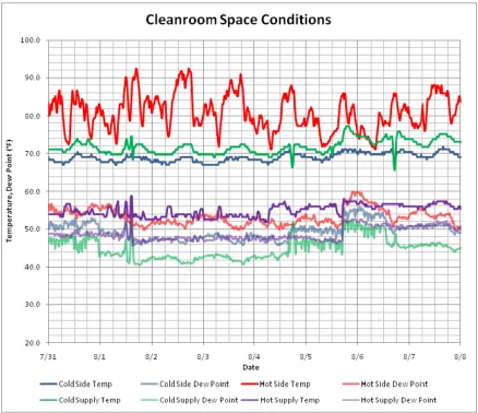
Figure 4.15: Cleanroom Space Conditions, August

(51)

40 Cooling Coils

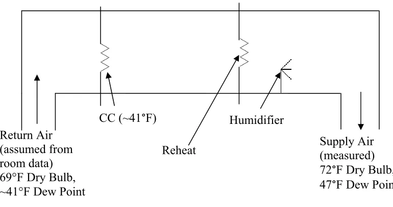
Figure 4.16: AHU 1 Energy Setup

Recall the Sample AHU Setup, Figure 1.5. This AHU looks physically like that one, but the assumed and measured temperatures have been added in Figure 4.16.

The real interest here is the difference between the cold supply dew point and the cold supply temperature. On the afternoon of 8/2, for example, the cold supply temperature is 72°F, while the cold supply dew point is recorded at 41°F. In Zone 1, therefore, there should be an astonishing 31°F of sensible reheat on approximately 45,000 cfm of air flow, with no heat recovery at all. If dehumidification is occurring as assumed, then the air leaving the cooling coil is saturated and 41°F.

The low dew point problem is addressed somewhat in Section 4.1.5. Even further though, when the actual loggers used were tested for dew point accuracy, the one logger which reads the lowest dew point by several degrees is the cold supply logger. It is worth noting that the temperature on this unit still reads accurately. Even if a dew point of 45-50°F is assumed there still needs to be a minimum of 21°F of sensible reheat on that large flow rate of air, or about 300 kW worth. The problem here is that AHU 1 records an almost constant reheat of 36 kW, not 300.

Reheat

Humidifier Return Air

(assumed from room data) 69°F Dry Bulb, ~41°F Dew Point

(52)

41

Recall how the cleanroom HVAC system is setup, from an energy standpoint. First, the air goes through the fan, and gets the fan energy added. Next, it goes through the cooling coils, and is cooled uniformly to the desired dew point, such as in Figure 4.16. This also takes out all of the added fan energy. Then, it goes through the reheat coils, and, if necessary, the humidifier. Therefore, the only source of heat for the cold supply in zone one is the cleanroom is the reheat on AHU 1. At a reheat of 36 kW, and for an assumed dew point/ leaving coil temperature of 45°F, the flow rate for zone one would be as follows:

36 3,413 0.24 72 45 4.2

122,868 6.48

0.075 60

4,210

(53)

42

40 3,413 0.24 72 69 4.3

136,520 0.72

0.075 60

42,140

This answer is almost right on the 45,000 cfm, considering the possible error in the

temperature data. However, this second situation comes with its own problems. First, supply temperature would then be warmer than existing room temperature. This would only be a plausible situation if the cold air from the hot supply area was making its way over to the cold side of the room. The only heat gains in zone are minimal (from the light and fan/reheat load), which is really the only way this could even be a plausible explanation. Below it is shown that in the adjacent hot zone, zone 2, AHU 2 has essentially no reheat. This may be unlikely, since the exhausted air is leaving from the hot side of the room.

In order to do these calculations, several assumptions have been made about the recorded data, which should be listed explicitly. First, it is assumed that the temperature data is correct. Although it was shown in Section 4.1.5 that there is a basis for doubting the dew point data, it has not been shown that there is any reason to doubt the temperature data. Secondly, it is assumed that the cold side room temperature is the same as the cold side return temperature. Third, it assumes that the fan load is around 4 kW, and does not take into consideration the possibility that fan load may not be measured, explained in Section 4.4. Finally, it also assumes that there is either cooling to the dew point (much cooling), or no cooling at all. There is no allowance for a small (but appreciable) amount of cooling. These may or may not be correct assumptions.

(54)

43

Figure 4.17: Cleanroom Cold Side Conditions, August

The figure above illustrates the position that the temperature for the cold side always stays between 2-4° F warmer than the supply. It is also shown that the supply temperature rises slightly more than that during the period between 8/5 and 8/11, which will be addressed later in Section 4.5. It also points to the possibility that there may be some small residual cooling, decreased by the higher chilled water temperatures. Another obvious curiosity is the

(55)

44

perfectly with raised supply dew point. One possibility is that this is functioning similarly to something mentioned in Section 4.1.4 with the AHU 4 reheats. Recall that since each reheat was operating at a different load, the total power (which is only measured on one leg) had the potential to be greatly misstated. The humidifiers are electric, and it is very possible that they could be staged by leg, instead of incrementally, and so therefore staged in a way hidden from the data logging equipment. However, without further proof, this is merely speculation.

Figure 4.18: Hot Side Overview, Winter

Figure 4.18 above shows some wintertime cleanroom temperatures. Note how the

(56)

45

more airflow. From this graph, days where the cleanroom are not in operation are visible as smooth ~65°F lines, such as Christmas week.

4.3 AHU Results

(57)

46

Figure 4.19: AHU Typical Reheat Operation, Summer

(58)

47

Figure 4.20: AHU Typical Total Operation, Summer

(59)

48

Figure 4.21: AHU Typical Reheat Operation, Winter

(60)

49

Figure 4.22: AHU 4: Total Power and Reheat

(61)

50

Figure 4.23: Winter Cleanroom Operation

(62)

51 4.3.1 The curious case of 9/22-9/29

On the morning of September 22nd, something happened to the operation of the cleanroom. This is illustrated perfectly by Figure 4.24 below. At around 10:15 AM on 9/22, AHU 3 reheat goes from an average of 73 kW to zero. Then, an hour and a half later, AHU 4 reheat goes from an average of 28 kW to zero. Suddenly, 101 kW of reheat just stops. At 7:15 AM the next day, the 100 ton compressor on Chiller 7 switches off. The outside temperatures during this timeframe are nothing unusual; they vary from the mid 70’s as a daytime high, to the upper 50’s as a nighttime low. The dew point, as shown on Figure 4.25, dips below 50°F on the afternoon of 9/22, but this does not seem unusual.

Then, even more suddenly, on 9/29 between 1:15 and 1:30 PM, AHU 1 reheat changes from being a constant 35 kW to oscillating between 0 and 70 kW. AHU 3 returns to the same pattern of operation it had before 9/22, and AHU 4 now operates between 65 kW and 0, oscillating. Before 9/22, the reheats averaged 135 kW. Afterwards, from 9/29 to 10/21, they averaged 148 kW. From 9/22 to 9/29, they averaged only 45 kW.

(63)

52

(64)

53

Figure 4.25: Outside and Plant Space Conditions, 9/22-9/29

(65)

54

Figure 4.26: 9/22-9/29: Hot Side Data

One interesting side effect of this weird AHU shutdown is the ability to do another energy balance. Looking closely at the time on Figure 4.26 before 9/22, the temperature is a fairly constant 53°F, with a constant reheat of 28 kW. Between 9/22 and 9/29, the temperature drops from 53°F to ~50°F, with no reheat. Then, between 9/29 to 9/30, reheat increases to 64 kW, and the temperature increases to 56°F.

(66)

55

28 3,413 0.24 53 50 4.4

95,564 0.72

0.075 60

29,500

While this number may seem to be lower than 45,000 cfm, keep in mind that it flow rates during this period may also have been disrupted.

64 3,413 0.24 56 50 4.5

218,432 1.44

0.075 60

33,710

(67)

56 4.3.2 AHU 2 Humidifier

Figure 4.27: AHU 2 Humidifier

(68)

57

of humidification is recorded. The humidification power, as listed above, is shown as if each of the three legs of power is drawn at the same amount. But it is very possible that this is not the case. This is why the total AHU 2 power can be zero while the reheat and humidifier show appreciable power draw. Also, the humidifier is apparently drawing power, but this does not seem to have too much of a humidification affect on the cleanroom (and is also puzzling).

(69)

58 4.4 Fan Results

Up until this point in time it has been assumed that the small ~5 kW in AHU 1, 3 and 4 was due to the fan load. This may not, in fact, be the case. The air handling units each have 100 hp fans (as we read from the nameplate) running on Variable Frequency Drives (VFD’s). At full load, these fans would draw 75 kW. The reheat on each unit totals a rated 70 kW, and the humidifiers are rated at 60 kW on each unit. In the electrical box for each AHU, there is a main three phase power, where each phase is split into three components. The largest three wires head to the fan, and the other wires go to the reheat and the humidification. These wires were traced to ensure accuracy of data logging.

Clearly, 5 kW is a small fraction of the maximum power used by the fans. This is such a low load that if accurate, the fans are probably not running on an efficient area of the fan curve. What is known is the relationship between fan speed, pressure and power. The flow rate through the AHU is directly proportional to fan speed (N). The pressure rise through the fan is a function of the speed squared. Finally, the power used by the fan is a function of the speed cubed.

4.6

4.7

4.8

If the power being utilized is 1/15th (6%) the motor power, the fan speed (and therefore flow rate) will be 41% of the maximum flow rate, and the pressure rise will be 16% of the

(70)

59

So what does all this mean? This means that if our readings are accurate (and correctly interpreted), the fans are grossly oversized for their current usage, and the design pressure rise is much larger than currently experienced. It also means that AHU 2 rarely runs a fan (as stated in Section 4.3.2), since it almost never has a total load.

Is there a case for the fans being oversized? Is there a reason it could have been designed that way? It is possible. The room may have been designed for larger flow rates for a higher cleanroom classification. After all, the chillers are oversized as well. Also, it may have been designed for a higher pressure drop across the HEPA filters, or a sizable cleanroom

pressurization level. This last reason seems most plausible.

Is there a case for the readings not being accurate (or correctly interpreted)? Unfortunately, there is. Undersized fans and pumps risk running in a very unfavorable area of their

performance curves, causing some problems. In addition, it is unusual for VFD equipped motors to receive power from a split power line. This is to protect the VFD against power oscillations from the other equipment (the VFD is expensive) and to protect the other

(71)

60 4.5 Chiller Results

In the graphs that follow, the chiller operation is detailed with respect to many parameters.

Figure 4.28: Chiller Power Consumption over Different Modes of Operation

(72)

61

8/15, the chillers have all 6 compressors running (all four circuits), although not completely loaded. The beginning of the graph (and the small period around 8/12) shows only 5 compressors operating (three circuits). Here, the 100 ton compressor on Chiller 8 is not operating.

Initially, it is important to remember that temperature, production, and cleanroom conditions all affect chiller power consumption. But for the moment, consider the changes taking place on the graph as if all of the other conditions are equal. Daily chiller power seems to ramp up very well, but then does NOT seem to ramp down very well at night. It is remarkable how the minimum power (except from 8/6 to 8/11) seems to find the same value night after night, even as the daily maximum varies wildly. Possible reasons for this include the following: temperature, humidity, production, cleanroom set points, and even chiller compressor limits. Considering the period where all 6 compressors are on between 8/1 and 8/5, the average chiller power use is 314 kW. The average for the period before this (7/29-8/1) is 293 kW, resulting in a net gain of 21 kW. Consider the period between 8/6 and 8/11. Here, the average use is 266 kW, a 48 kW decrease over the previous period, and the average power use for time after 8/12 is about 288 kW.

(73)

62

Figure 4.29: Cleanroom Chilled Water Temperatures, August

(74)

63

Figure 4.30: Cleanroom Chiller Power, July

(75)

64

Table 4.1: Chiller Power Totals Timeframe of Average # of Averaged Data Points Chiller 8 (kW) Chiller 7 (kW) Total (kW)

6-19 to 6-25 874 71.1 169.1 240.3

6-25 to 7-1 808 121.6 168.7 290.3

7-1 to 7-6 743 87.9 158.2 246.2

7-6 pm to 7-7 pm 149 3.2 216.9 220.1

7-7 pm 21 2.3 307.5 309.7

7-7 pm to 7-8 am 66 102.2 247.8 350.0

7-8 to end 2,506 120.4 166.5 286.9

Total/ Average 5,167 103.5 169.2 272.6

(76)

65

Figure 4.31: Cleanroom Chiller Power (Single Week)

This single week chart is provided to illustrate the strange chiller behavior on the afternoon of July 7th. For all of the data before and after July, sustained chiller power spikes on either chiller are a function of any one of the four chiller circuits coming on or off, and also

(77)

66

However, this possibility is tempered by the next jump in data, in the early hours on July 8th, in which the single compressor circuit on Chiller 7 suddenly drops 40 kW, with a small reaction from Chiller 8. Obviously, the single compressor cannot shut halfway off, so this change was probably done with controls, since it is unlikely that the chiller is being tweaked at 2:30 am.

So what was happening with respect to outside operating conditions?

Figure 4.32: Temperature and Dew Point with Chiller Power (One Week Graph)

(78)

67

power use is below that which would be expected, given the performance data for the week previous. Yes, the humidity is down overall, but the humidity is comparable in the early hours of 8/10 to the early hours of 8/4, and power use is still way down.

(79)

68

Figure 4.34: Chiller Power and AHU Power

In Section 4.2, it was mentioned that decreased production could be the cause for slightly higher reheat usage at night. If this is the case, then could it be possible that the daily

increase in chiller capacity is related to the cleanroom production? On 6/22, for example, the daily change in chiller power is 100 kW. The daily change in reheat over that period is 70 kW. However, the cooling effect the chiller is having is greater.

100

1.25 12,000

1

3,413 281 4.9

(80)

69

large swing, and on some days, the swing is nearly random. The averaged on peak increase in chiller power over that period is 52 kW, while the average increase in on peak reheat is 14 kW. That is only 9.5% of the energy, so there exists the possibility that this relationship may be lost in the data, so to speak.

Figure 4.35: Cleanroom Chiller Power (6/23-6/29)

The chiller power of units 1-5 are almost completely production based. There are large users of chilled water which may demand chilled water at anytime, which helps explain the

(81)

70

rooftop units, so any daytime load should act independent of outside temperature, and rather as a function of increased daytime work activity. But as the graph shows, it clearly appears to be a function of outside temperature.

Why could this be the case? It could be the case that there are several small A/C systems which actually do draw from the chilled water loop. However, to cause 50-100 kW changes in demand, these must be 40-80 tons of A/C capacity. This does not seem too likely. The other possibility is that the increase in daytime drybulb temperature is lowering the

(82)

71

Figure 4.36: Cleanroom Chiller Power (9/13-9/26)

(83)

72

Figure 4.37: Chiller Power and Outside Temperature, November

(84)

73

Figure 4.38: Chiller Loads and Outside Conditions

(85)

74

Chapter 5: Analysis

Figure 5.1: Cleanroom Temp, AHU Power, and Cleanroom Chiller Use

It was explained above that the cleanroom has about 5,000 cfm of outside air entering the AHU’s. As explained in Chapter 6, this amount has been increased to a measured 15,000 cfm, in order to pressurize the cleanroom to about 0.5 inches Hg, which has now been achieved. (Although the outside air flow has been increased by threefold, it does not follow that the energy required to condition it also increases threefold. See Chapter 6 for

(86)

75

50°F. The cold side supply temperature is a balmy 70°F, and has a supposed dew point of 42°F. Since this is going to be a conservative calculation for the maximum possible

infiltration load, it will be assumed that the air is all cooled to the cold side dew point (42°F is too low, so 48°F will be assumed), and then reheated. Thus, an enthalpy of saturated air at the cold supply dew point of 19.2 BTU/lb will be assumed.

5,000 0.075 60 37.4 19.2

5.1

409,500

12,000 1.25 /

42.7

(87)

76

Is this a one day phenomenon? No. This happens day after day, month after month. This points to one problem in particular: condenser heat transfer. It could be that this is merely a consequence of design, and as the outside air temperature increases, there simply is not enough heat transfer space to compensate for without increasing the temperature difference. This would be done by increasing the pressure and temperature of the refrigerant, and as a consequence lowering the COP of the chillers.

There could be a much more mundane cause, however. The plant already has a scheduled program to clean the outside heat transfer surfaces on all of their chillers. Are the heat transfer surfaces inside the chillers periodically checked for sludge buildup?

(88)

77

Figure 5.2 shows a graph of chiller power vs. outside temperature. The 7 data points on the graph each average at least a week of data, to try and eliminate short term variables which may confuse the relationship. The minimum chiller load appears to be 120-130 kW. This relationship will be used to try and estimate a total cost of running the chiller in a typical year.

Figure 5.3: Average Power and Average Outdoor Temperature

(89)

78

The actual cleanroom data from July is shown in Table 5.1 below. Table 5.1: July Chiller Power Cost

Daily Data Averages Sum Monthly Average _{Percent Cost} Understatement Energy / Power Cost Energy / Power Cost

($) ($) (%)

Offpeak 148,360 kWh $4,052

200,758 kWh $6,344

Onpeak 52,398 kWh $2,375

Energy Subtotal 200,758 kWh $6,427 200,758 kWh $6,344 1.3% Demand 372 kW $3,732

279 kW $2,797 25.1%

Max Demand 467 kW $4,688 40.3%

Total Cost $10,159

$9,141 10.0% Max Total Cost $11,115 17.8%

In Table 5.1, it is shown that the average kW draw in July was 279 kW. However, the maximum daily on peak average was 372 kW, and the maximum 30 minute average demand was 467 kW! It is likely that that hot summer day set the peak at the facility. To be

conservative, assume that the demand is only 372 kW. This demand figure is 25% more costly than the average demand would cost, and 10% more costly overall. This is typical of all the summer months, and this is actually more extreme in the winter, since daily maximum chiller power use can peak at over 200 kW.

From historical weather data, average monthly temperatures can be found for the site. An average temperature in the upper 70’s corresponds to 270-280 kW average power draw. An average temperature of 45-50°F corresponds to an average power draw of 150 kW,

(90)

79

Table 5.2: Extrapolated Chiller Energy Cost

Energy Energy Cost Demand Demand Cost

(kWh) ($) (kW) ($)

Summer (4 mo.) 784,800 $24,800 1,090 $13,500 Winter (8 mo.) 892,800 $27,700 1,240 $8,500

Total 1,677,600 $52,500 2,330 $22,000

In the table above, the total cost comes to $74,500/yr. Note that a 25% demand surcharge on all the extrapolated demand figures.

So what should the chiller system need to provide? The heat load in the cleanroom now would need to be roughly estimated. If this load is ~400 kW, and the typical daily maximum summertime infiltration load is 42.7 kW (from earlier in this section) the maximum amount of energy the chiller should have to remove is around 440 kW (1,500,000 BTU/hr), which is roughly equivalent to 150 kW of chiller power at 1.25 kW/ton.

The possible potential for chiller power savings is up to 150 kW of summer load shedding, depending on the internal heat generation of the cleanroom. Unfortunately, since it has been shown that the chillers do not efficiently handle high outdoor temperatures or low loading, the easiest part to concentrate on is eliminating reheat.

(91)

80

Table 5.3: Extrapolated Reheat Energy Cost

Energy Energy Cost Demand Demand Cost

(kWh) ($) (kW) ($)

Summer (4 mo.) 345,600 $10,900 480 $4,800 Winter (8 mo.) 338,400 $10,500 470 $2,400

Total 684,000 $21,400 950 $7,200

This is seen to total $28,600/yr from the table above. In direct chiller savings, at 1.25

kW/ton, it would save 43 kW of load from the chiller in a summer month, and 18 kW of load in a winter month.

(92)

81

Chapter 6: New Cleanroom Operation

6.1 New Cleanroom Operation Overview

The company is hitting this problem from multiple angles. In Chapter 4, it was discussed that several things can be done to help the cleanroom operate more efficiently, largely with the same equipment. This chapter will explore the things the company is currently doing to discover the potential of the measures. Recall from Chapter 1 that the cleanroom is currently taking in 5,000 cfm of outside air, equally spread across AHU’s 1-4. Now, the plant wants to change how the AHU’s operate. The plant wants to utilize AHU’s 2-4 as filters and

temperature control alone, hoping to completely eliminate reheat on these three units.

AHU 1 will now take 15,000 cfm of outside air to pressurize the cleanroom, and not condition any return air. Note that this is an additional 10,000 cfm from the previous operation. This AHU will be utilized to control humidity, and therefore will potentially operate at a different temperature from the other units, depending on cleanroom conditions. Humidification by AHU’s 2-4 still may be necessary during cold or dry periods.

Should the latent cooling load be too much for AHU 1 to handle, it is recommended that one other AHU (say, AHU 4) be used for dehumidification, in a periodic manner. Should this need to happen, it is also suggested that sensible cooling be lowered dramatically on AHU’s 2 and 3 to minimize the amount of reheat required. This should be rare, however. Since the new cleanroom operation eliminates all possible sources of outside infiltration (other than AHU 1), the only possible way this should be required is by an increase in internal humidity generation.

(93)

82

(94)

83 6.2 AHU 1 Modifications

The plant currently has about 6,000 cfm of exhaust as hot contaminated air leaving the cleanroom through roof vents. An air to air heat exchanger has been installed in this air stream to preheat the incoming outside air in the winter. The design HX effectiveness is 63.4%, and it is estimated to be is use when the outside wetbulb temperature drops below 57°F. It has the ability to increase the temperature of the incoming 15,000 cfm of air by 25°F, illustrated by example air temperatures in Figure 5.1 below. In addition, if the outside air is too cold, AHU 1 has the capability to draw plant air as makeup as well, in order to avoid electric strip heat. The plant has a gas heating system, and with natural gas running between $5-$10/MMBTU, it is preferable to utilize the plant heating system. Since the cleanroom will now be pressurized, it provides conditioned air to the plant through