ABSTRACT
PROPST, MICHAEL DAVID. Applying Linear Regression and Neural Network Meta-Models for Evolutionary Algorithm Based Simulation Optimization. (Under the direction of Dr. Jeffrey Joines.)
The advances in computing power over the last decade have led to an increase in the use of
simulation programs and their complexity to model real world optimization. An
experimental design is often used to determine the effects varying parameters have on the
desired output. The user is usually trying to optimize or minimize a series of outputs.
However, these problems often have a large number of variables or parameters that can be
changed with a wide range of values increasing the complexity of the model. As these
simulation models become more complex they become computationally expensive to run.
Most of these problems are non-linear and based on the inherent variability in real-world
applications and may not have a true optimal solution. Evolutionary algorithms are a class of
computational optimization techniques that are based on the principles of evolution and
harness the power of the computer to solve a problem. The application of evolutionary search
techniques as a simulation optimization technique has yielded promising results. However,
the algorithm can take a long time evaluating just one set of decision variables owing to
replications and computational time of one simulation run and not to mention the sheer
simulation model. Therefore, this thesis combines the use of evolution algorithms, simulation
models and meta-models to produce a more efficient simulation optimization technique.
The two types of meta-models are tested to determine their effectiveness as a meta-modeling
Applying Linear Regression and Neural Network Meta-Models for Evolutionary Algorithm Based Simulation Optimization
by
Michael David Propst
A thesis submitted to the Graduate Faculty of North Carolina State University
in partial fulfillment of the requirements for the degree of
Master of Science
Textile Engineering
Raleigh, North Carolina
2009
APPROVED BY:
_______________________________ _________________________________
Dr. Jeffrey A. Joines Dr. Timothy Clapp
Committee Chair
DEDICATION
I would like to dedicate this paper to Jon Rust. A man whose influence on my life I could
not begin to explain. He found a confused boy and worked tireless to unlock his potential
and had faith when others didn’t. Without whose small but effective words of motivation I
would have never considered graduate school yet alone coming back to complete this project
four years later. His guidance I am grateful for, inspiration I am thankful for, and his
friendship I will always cherish.
I would like to thank Jeff for having patience and not giving up when others would have and
digging into the archives to finish this.
And to mom….well for being mom and always understanding and but somehow pushing.
BIOGRAPHY
Michael David Propst – was born in North Carolina and raised in Concord. He found his
way to NC State via Northwest Cabarrus High School. He received his B.S. in Textile
Engineering from North Carolina State University in Dec of 2002. He then proceeded
directly to work on his M.S. in Textile Engineering from the same university. Upon
completion of his coursework he began working for Abercrombie & Fitch Trading Company
as a Quality Engineer. During which time he spent numerous months in South Asia and
South East Asia in garment production optimization eventually completing his M.S. thesis in
ACKNOWLEDGMENTS
I want to acknowledge Dr. Jeff Joines who helped guide me through this journey and was
with me every step of the way; especially the late steps.
I would like to thank Angie Brantley who made sure all of my paperwork was submitted
properly and on-time. She was instrumental as I was not in NC during the completion of
this.
I would like to thank my committee members who were exceptionally patient with the
constant rescheduling and for Dr. Thompson who came on at the end when we needed his
TABLE OF CONTENTS
LIST OF TABLES ... viii
LIST OF FIGURES ... ix
1 INTRODUCTION... 1
1.1 Opportunity ...3
1.2 Approach...4
2 LITERATURE REVIEW ... 7
2.1 Simulation ...7
2.2 Simulation Optimization...9
2.2.1 Simulated Annealing ...11
2.2.2 Particle Swarm Optimization Method ...11
2.2.3 Genetic Algorithms ...12
2.2.4 Stochastic Approximation ...12
2.2.5 Models of Simulation Models (meta-models) ...13
2.2.6 Response Surface Methodology ...13
2.3 Genetic Algorithms ...18
2.4 Meta-model ...23
2.4.1 Stepwise Regression...23
2.4.2 Neural Network ...24
2.4.3 Neural Network Training ...26
2.5 Simulation Optimization – Why we need meta-models ...28
2.6 Approach...29
3 DETERMINISTIC EXPERIMENTAL PROCEDURE... 31
3.1 Experimental Setup...34
3.1.1 Experimental Parameters...35
3.1.2 Experimental Procedure Step-by-Step...39
3.2 Experimental Design ...41
3.3 Output Data ...43
3.4 Results ...43
3.4.1 Neural Network ...44
3.4.2 Regression ...58
3.5 Neural-network Model versus the Regression Model ...61
3.6 Discussion...65
4.1 Goal ...66
4.2 Experimental Setup...68
4.3 Experimental Parameters...69
4.4 Experimental Design ...71
4.5 Output Data ...72
4.6 Results ...73
4.6.1 Schwefel Function ...73
4.6.2 Model Accuracy ...77
4.6.3 Number of Generations for Best Solution ...82
4.7 Experiment to test solution quality v the iteration of the solution ...87
4.8 Conclusions ...88
5 CONCLUSIONS AND FUTURE WORK ... 89
LIST OF TABLES
Table 3.1: Parameters and Settings ... 38
Table 3.2: Neural Network Parameter significances (significant parameters high-lighted in yellow) ... 45
Table 3.3: Least Sq Means Table – Schwefel Function... 52
Table 3.6: Brown Least Sq Means ... 56
Table 3.8: Quantile Analysis of Regression Modeling Technique ... 58
Table 3.9: Regression Significance (significant values high-lighted in yellow) ... 59
Table 3.10: ANOVA Values for Retrain ... 60
Table 4.1: Parameter Levels ... 70
Table 4.2: Schwefel Significance Values ... 73
Table 4.4: Corana 10 variable Student T means analysis ... 77
Table 4.5: Mean Comparison... 77
Table 4.6: R-squared Values of Estimate & Actual Correlation ... 78
Table 4.7: Schwefel Est v Actual differnece Quantitiel analysis... 78
Table 4.8: Best Solution Quantile Analysis - Schwefel... 79
Table 4.9: Best Solution Quantile Analysis – Brown ... 80
Table 4.9: Best Solution Quantile Analysis - Corana ... 81
LIST OF FIGURES
Figure 2.1: RSM Method (Taken from Neddermeijer et al (2000)) ... 17
Figure 2.2: A Simple Genetic Algorithm... 20
Figure 2.3: Least Squares Equations for Linear Regression Model (Wackerly 2002) ... 23
Figure 2.4: Basic Neural Network ... 25
Figure 3.1: Schwefel and Brown Function Equations and Optimal Values ... 32
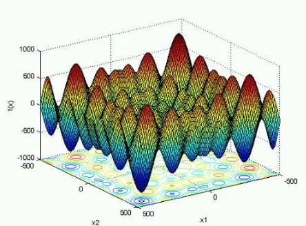
Figure 3.2: Schwefel Response Surface for nv=2 [Ifram] ... 32
Figure 3.3: Brown’s Almost Linear Function [Humphrey, 2000] ... 33
Figure 3.4: Step-by-Step Procedure: No Retrain ... 40
Figure 3.5: Step-by-Step Procedure: Retraining Between Search Replications ... 40
Figure 3.7: Schwefel Effect Analysis ... 48
Figure 3.8: Brown Effect Plots ... 55
Figure 3.9: ANOVA for Retrain ... 60
Figure 3.10: ANOVA for Neural-Network v Regression ... 62
Figure 4.1: Corana Function Equation... 67
Figure 4.2: Corana Function Plot – n=2 ... 67
Figure 4.4: ANOVA Noise Level ... 76
Figure 4.5: ANOVA for Parameters – Schwefel ... 84
Figure 4.6: ANOVA for Parameters – Brown ... 85
1
Introduction
Maximizing resources and/or minimizing costs are essential for any company to excel in the
increasingly competitive international economy. In designing, creating and/or improving a
product or process of any sort it is important to be able to optimize the system or product
with the appropriate set of inputs to increase the profitability of the product. Also, “any
abstract task to be accomplished can be thought of as solving a problem, in turn a search
through a space of potential solutions.” [Michalewicz, 1996] Examples can range from
determining the optimal set of parameters for a series of machines to produce the best quality
for a given price, designing the optimal layout of a manufacturing floor or airport to
optimizing a 401K portfolio so one can retire earlier.
The output of these processes commonly relies on many variable inputs that are often
interdependent with one another and can range from discrete to continuous inputs, to
qualitative inputs, to statistical distributions. Many of these systems to be optimized do not
have a closed form (i.e., a set of equations to optimize) owing to the complexity of the
system. Computer simulation is commonly used to predict the output of these processes.
This involves developing a model of the system in a simulation modeling language that takes
the inputs that drive the particular process and produces a series of output metrics of the
people, baggers, etc.) or stochastic. Stochastic inputs (e.g., processing times of jobs at a
machine, the time between arrivals, the number of items selected at a store, the number of
people who arrive at a store) are random and occur based on a distribution. These inputs
increase the complexity of the simulation. For example, consider a grocery store simulation
where one is trying to determine the optimal number of baggers and checkout clerks needed
during each time period the grocery store is open. A model of the system can be developed
by determining the statistical distributions of the arrival rate of customers to the store, the
length of stay, the check out processing times, the number of items purchased, etc. Executing
the simulation model can take a substantial amount of time when replications are required;
which is common when dealing with stochastic simulation models to produce a more
accurate picture of the true outcome. Therefore, it is often the case that only a few different
sets of inputs are tried and the best system is taken from this subset. In order to maximize the
efficiency of a process, simulation is commonly used in conjunction with single variable
experimentation, which entails changing one variable at a time and observing the output.
This method of experimentation is devoid of intelligent planning and any explanation of
interaction effects of any order. This method also limits the search space to that conceived
by the searcher and thus based on experience, intuition, or more commonly no data at all.
Very little research has been performed in optimizing simulations as opposed to general
mathematical models since no closed form exists. It is impossible to generate search
do not work in this arena due to the stochastic output. Genetic Algorithms(GA) are a part of a
field of computational optimization methods that do not rely on gradients to perform the
search and are independent from the evaluation function in making search decisions. These
algorithms are known for their ability to search a large search space very efficiently
consisting of hundreds or even thousands of variables to achieve an optimum solution. This
technique utilizes evolutionary techniques that mimic natural evolution, which include
random mutation, simulating mating or crossover, and survival of the fittest. This enables
the program to converge to an “optimal solution” while thoroughly exploring the solution
space. The term “optimal solution” is meant to represent a very good point, which may or
may not be the true optimal of the system due to the nature of GAs.
1.1
Opportunity
Researchers have used various techniques to determine the best set of inputs that will
optimize a computer simulation, which in term should optimize the true system [Androitter
1998]. These have been found to be effective in computing a good solution for the
optimization of the process. The genetic algorithm can be thought of as a directed random
search and during the search process it often creates children (i.e., new solution points) that
are poor or away from the best solution (i.e., creating random points to drive the search).
simulation computationally expensive to determine the optimum of the system. Also, in order
to limit the stochastic nature of the output, the simulation is run multiple times for a
particular set of variable inputs into the simulation which produces a stochastic output to find
a value closer to the mean and thus increasing the evaluations of a single point. The GA
maintains a population of solutions which can be thought of as short term memory since this
represents a small snapshot of the space which can be lost from generation to generation.
There is an opportunity to increase the computational efficiency of the program by
creating a mathematical model of the search space from either the historical data (i.e.,
starting population) or a planned experiment. Creating a mathematical model of the process
from the data to some degree of error will allow a simple mathematical equation for the GA
to optimize which will dramatically decrease the amount of computational effort needed to
evaluate an individual in a population.
1.2
Approach
The goal is to determine the most efficient way to optimize a simulation model utilizing a
meta-model. The approach will determine the best way to determine the meta-model and how
to combine it with the actual simulation model and genetic algorithm.
There are many methods available that generate a mathematical model from a data set
containing explanatory variables and their outputs. This data can commonly come from
Some of these techniques output a linear model, such as ordinary least squares regression,
and some produce a non-linear model, such as neural network modeling techniques. The
goal of this research is to fuse one or more of these modeling techniques with the simulation
and genetic algorithm searching techniques. These modeling techniques will be used to
create a model of the simulation solution data space, or meta-model, which the genetic
algorithm searching technique will use to evaluate some of its new solution points. This will
give a rough estimate as to the quality of this solution and it is a cheap and inexpensive way
to determine if a new solution point should be kept in the population. Even a slight decrease
in the amount of simulations that have to be run to complete the optimization can
dramatically decrease the amount of time necessary to run the optimization. When should
the meta-model be used for evaluation? How often should it be used for evaluation? Under
what circumstances should the meta-model be used? Which modeling technique is best?
Which modeling technique produces the least error? These are all questions that the
research will attempt to answer.
Numerous approaches exist that can be used to create a model for the genetic algorithm
to work on. There also many questions associated with these techniques. These questions
will be discussed with each technique in Chapter 2. The approaches explored in this paper
pertain to the fields of statistical theory and neural computing. Many options and techniques
in statistical theory are explored along with a back propagation technique derived from the
meta-models that are created through an adopted stepwise regression program as well as a back
propagation neural networking algorithm. These algorithms are executed on both
deterministic and stochastic optimization problems of varying complexity. Chapter 5
summarizes the findings including ideas for further research and suggestions upon the
2
Literature Review
The computationally expensive nature of simulations involving a large number of input
variables has fueled the proposition of many different methods for determining the optimal
values for those input variables to find the best solution. Different modeling techniques exist
as a means to replace the computationally expensive simulation with an analytical based
model representation. This would allow the model to be accessed as opposed to the
simulation itself, thus higher sampling optimization methods to be utilized can properly
explore the possible solution space.
2.1
Simulation
Simulation is a powerful tool used for modeling complex systems. It is used to model new
system designs, proposed system changes, and retro-fitting existing systems. Simulation is a
tool for aiding decision-making. A simulation model represents time and changes that occur
in the system or process over time. The majority of simulations are discrete, meaning that
changes occur only at discrete points in time; which is in contrary to continuous simulations
where changes occur continuously. Discrete event simulation models are less complex than
continuous simulation and easier to model. Discrete event simulation models are based on
concepts of events, activities, processes, and states; which are commonly explained as events
commonly represented by a vector containing variables that describe the state of the system
at any time. This vector is referred to as the model state [Carson, 2004].
Similar to other sciences, computer simulation contains its own vocabulary. An event
is an occurrence that changes the models state instantly [Carson, 2004]. An example of an
event is the arrival of a customer at a checkout lane in a grocery store. An activity is a
duration of time, such as the amount of time necessary for the checkout clerk to total the cost
of the customers good. Events and activities are commonly modeled using a probability
distribution derived theoretically or from historical data [Carson, 2004]. Distributions that
can commonly be applied to discrete simulation are the Gaussian (Normal), Poisson, and
Geometric distributions. Entities in simulations are objects in the model. Dynamic entities
refer to entities created at time points, such as the completion of a customer check-out.
Resources provide services to dynamic entities, such as checkers, baggers, etc. Simulations
commonly contain stochastic inputs, such as the arrival of customers to a grocery store and
the amount of time that they spend shopping before proceeding to the check-out. These
inputs are modeled using a probability distribution. These variable stochastic inputs generate
a variable stochastic output, creating a distribution or any single configuration of the system
or process [Carson, 2004].
Simulation models are used to represent a number of different system or process
configurations. This is done by varying the input parameters associated with the simulation
These models can be used to determine the best configuration of the output parameters over
the finite sets of configurations. However, the size of the input parameter space, the number
of variables, the range of those variables, and the types of variables can make a trial and error
method ineffective.
Since simulations are used to model processes that cannot be modeled analytically it is
necessary to seek out an alternative way to optimize the simulation. Simulation optimization
refers to the search for the combination of configurable variables to maximize or minimize
the desired output. This output is commonly the performance of the system or process. Such
complex problems are commonly found in manufacturing and supply chain management.
The stochastic nature of such problems prevents simple analytical modeling and optimization
techniques [Olafsson 2002].
2.2
Simulation Optimization
Simulations are a tool to aid in decision making; not a decision making tool. They are
considered a tool to answer “What If” questions [Magoulas 2002]. Simulations can be used
to determine the state of controlled inputs and their effects on the output [Bowden 1998].
Simulation optimization can be viewed as finding a combination of input parameters that
yields the greatest output [Humphrey]. In order to achieve this optimum output a simulation
parameters. Stuckman et al (1991) divide simulation optimization into three categories. The
first being one that utilizes “trial and error” methods. This is randomly varying inputs in an
effort to achieve a better performing outcome. The second is systematically varying
parameter input and observing the effect on the output (e.g., design of experiments, response
surface methodology (RSM)). The goal is to ascertain some correlation between the input
changes and the final outcome. The third category is an automated simulation optimization
approach [Magoulas 2002].
Discrete decision variables refer to the system or process whose sample space is
finite. The optimization methods for discrete decision variables are dependent of the size of
the variable space and the complexity of the problem. This is normally determined by
whether or not it is feasible to simulate the entire sample space. It is quite common that it is
impossible to simulate the complete sample space. For the problems where it is impossible
to simulate the entire sample space a technique must be employed to determine which points
to sample and thus simulate. Subset selection or screening attempts to reduce the feasible
region so as to make it more manageable during the optimization process. If the output space
is large and complex then the previous two methods fail to adequately explore the sample
space and thus fail to provide a solution with reasonable confidence [Olafsson].
Considerable research has been done in the third category. The ever increasing
complexity of simulation problems in conjunction with increasing computing power allow
stochastic component to prevent the search algorithm from getting stuck in local minimum/
maximums. With stochastic based search operators there is no guarantee of finding the true
optimal value; only a potentially good one. There are a number of computational
optimization techniques (random restart, response surface methodology, Simulated
Annealing, Genetic Algorithms, Particle Swarm Optimization, Stochastic Approximation).
2.2.1 Simulated Annealing
This method is inspired by the thermodynamics process of annealing of metals in physics
where metal is cooled, reheated, cooled again, etc. to reach the minimum equilibrium state.
Simulated annealing explores solutions in a neighborhood and evaluates their fitness. The
program is allowed to search for solutions in neighborhood of a lesser value. This prevents
the method from converging on a local minimum. Whether or not the lesser valued
neighborhood is explored is based on a function utilizing a random number and the amount
of time it has been searching. The longer the algorithm has been searched the less likely it is
that it will be allowed to explore the lesser valued neighborhood [Avello 2004].
2.2.2 Particle Swarm Optimization Method
Particle swarm optimization is another computational probability meta-heuristic that mimics
the behavior of a “bird’s flock” in that social information sharing takes place. Individuals
can profit from their own experience as well as those of the other solutions in the “swarm”.
as well as the experience (i.e., direction) from other potential solutions in the “swarm”
[Magoulas 2002].
2.2.3 Genetic Algorithms
Genetic algorithms (GAs) mimic Darwin’s evolution process to move throughout the space.
Since this study utilized this meta-heruistic as the global optimization strategy it will be
discussed in detail in Section 2.3.
2.2.4 Stochastic Approximation
Stochastic approximation is the process of moving in the direction of greatest ascent. There
is no analytical function from which to determine this direction, thus the gradient is estimated
by choosing points at a finite distance form the current solution in the solution space to
approximate the gradient. These points can either be chosen in a single variable direction to
the current solution and the gradient projected in the other direction or points can be chosen
from both sides. It has been proven that stochastic approximation will converge
asymptotically given certain conditions and a sufficiently slow decrease in the step size. A
draw back to this method is that with each step of the stochastic approximation, n+1
methods are not limited by the constraints of the input parameter space; i.e. the number of
baggers available at a grocery store can only be a whole number.
Optimization methods vary depending on the complexity and type of configurable
variables available for optimization. Gradient search methods, such as Response Surface
Methodology and stochastic approximation, are commonly used for continuous variables.
For finite and small systems ranking and selection methods may be used and for finite and
large systems a metaheuristics should be applied [Olafsson 2002]. A metaheuristic is a
non-analytical method of solving a problem that involves one heuristic driving a lower level
heuristic or set of rules, to move throughout the search space.
2.2.5 Models of Simulation Models (meta-models)
These previous computational methods require a large amount of simulations in order to be
effective which is why they are often used in deterministic optimization. In order to allow
optimization techniques to work efficiently, a model of an initial output dataset is
constructed. This is referred to as a meta-model (see Section 2.4 for more information) and it
simplifies the simulation model itself, exposing the fundamental nature of the system input
and output relationship [Santos, 1999]. This model can then be acted upon by the
optimization method.
2.2.6 Response Surface Methodology
Response Surface Methodology (RSM) appears to be an obvious choice for creating a
statistical methods utilized for experimental optimization as stated by Joshi et al [1998] in his
paper describing an enhanced RSM algorithm. RSM incorporates gradient deflection
methods and restart criteria as opposed to the traditional method of utilizing steepest ascent
or descent direction. They describe the conventional method of RSM as initiating the
described method by performing an experimental design in a small sub-region of the
available space and modeling the data with a low degree polynomial. The method then
proceeds to climb down the response surface. The typical RSM stops when the response
either moves opposite to the desired direction or shows no further improvement. This
method works under the assumption that the true optimum can be obtained on this path thus
having very limited exploration. At this point, another experimental design is conducted to
determine curvature and create a two degree polynomial analysis. A canonical analysis is
then conducted to determine if further exploration needs to be conducted. Next a ridge
analysis may be performed to collect observations along the ridge direction. From here the
analysis may continue using discrete step sizes to determine “the optimal” in that region.
The method relies on a random restart or multi-start technique to explore the experimental
space [Joshi, 1998].
The Enhanced RSM Algorithm introduced by Josh et all (1998) initializes at a random
point as well as treats this point as the incumbent solution. A 2K factorial experiment is
constructed with the incumbent solution at the center. The path of steepest descent is
violate the bounds of the experiment. Following determination of the appropriate step
length, a second order model is created. After the model is checked for adequacy, a
canonical analysis is performed. Then the algorithm is repeated until the termination criteria
are met. The can be either a set of predetermined criteria or no further improvement is
commonly used [Joshi, 1998].
Neddermeijer et al (2000) created a framework for a fully automated RSM
framework. A graphical representation can be seen in Figure 2.1. The framework initializes
with a given starting point and step size. From the initial point, the response function is
modeled using a first order model which is then tested for adequacy. Should the model not
have a significant ability to predict the data, then the steepest descent direction cannot be
determined. A line search is performed in the area of the steepest descent. The
predetermined step size is taken in that direction. This is the optimum for the nth iteration of
the framework. The line search is continued in that direction until the stopping criteria has
been met. Other options that take the noise of the model into consideration stop when two or
three consecutive points in that direction continue to achieve less desirable solutions. Should
the first order model be found inadequate and there is evidence of pure curvature or
interaction effects, a second order model can be applied to increase the accuracy of the
model. To maintain the efficiency of the framework is has been found beneficial to reduce
Once the termination criterion has been met, the new region of interest is represented
by a second order model which is also tested for adequacy. Again, if the model is found to
be inadequate, the size of the new region of interest can be reduced by reducing the step size.
Should the second order model be found to be adequate, a canonical analysis is performed to
determine the nature and location of the current optimal solution. Then a ridge analysis is
performed if the current optimal solution is found to be a saddle point [Neddermeijer 2000].
Ridge analysis computes the estimated ridge of optimum response using increasing radii
from the original data point. The direction of steepest descent is determined for the second
order model and a line search is performed in that direction. Once the optimum point in this
new direction is found, the algorithm is repeated until an optimum solution is found
RSM provides a logical way to search for an optimal value for an experiment with
variability. RSM relies on a computational optimization technique called random restart to
fully explore the sample space. RSM depends on the linearity of the problem being
optimized which presents a weakness in the method. RSM optimization depends on the
ability to create both first and second order equations on the sample space as well as the
ability to create differential equations from the derived models. This presents a problem in
the goal of a completely automated program.
2.3
Genetic Algorithms
Complex problems like supply chain optimization are very difficult to solve. There is often
no underlying analytical model and often a nonlinear relationship between the variable(s)
being optimized and the prediction variables. This, coupled with the size and complexity of
the search space, creates a seemingly impossible problem. Genetic algorithms have been
shown to produce good results for a wide range of problems though the use of their powerful
global search techniques based on Darwin’s theories of survival of the fittest and random
mutation. Genetic algorithms both explore the sample space and exploit promising areas
exponentially. This is accomplished through mutation, crossover, and selection operations.
This improves the overall strength of the population in successive generations and focuses on
the most promising solution space. Due to the stochastic nature of the crossover and
mutation procedures, weak individuals or children will be created. These individuals add to
the explorative properties of the algorithm. They are not detrimental to the overall strength
of the program since they are removed through the selection process during subsequent
generations. If a weak solution should survive a generation, it will eventually be removed
and thus not cause serious damage to the algorithm or hinder the final solution. The next
generation of the population is created through random methods and evaluated by
comparative selection based on a random underlying pairing. This differs from traditional
optimization methods which are based on predetermined decision rules. Genetic algorithms
do not make strong assumptions about the form of the objective function; thus allowing them
to operate on a large range of problems [Joines 2002]. The general genetic algorithm is
1. Set generation counter i ← 0.
2. Create the initial population, P0, by randomly generating N individuals.
3. Determine the fitness of each individual in the population by applying the objective function to the individual and recording the value found.
4. Increment to the next generation, i ← i + 1.
5. Create the new population, Pi, by selecting N individuals stochastically based on the
fitness from the previous population, Pi−1.
a. Randomly select R parents from the new population to form the new children by application of the genetic operators.
b. Evaluate the fitness of the newly formed children by applying the objective function.
6. If i < the maximum number of generations to be considered, go to Step 4. 7. Output the best solution found.
Figure 2.2: A Simple Genetic Algorithm
The solutions, or individuals, in the population are described by a chromosome
representation consisting of a vector representing the predictive variables. The algorithm is
initiated by creating an initial population and then evaluating their fitness to the objective
function. A subset of the population is then selected to parent the next generation. It is
possible for an individual to be selected to parent more than one offspring. Either crossover
or mutation is performed to create the offspring. For example, one crossover consists of
randomly selecting a cut point on the parents then swapping the numbers after the cut point
between one another creating two distinct children. Crossover combines traits from both
parents to create the new children. Mutation occurs when a random individual is selected
and a random chromosome change is performed. The goal of mutation is to inject new
either arbitrarily or by selection methods, such as ranking, binary selection, etc.
[Michalewicz]. Genetic algorithms have successfully been used to solve a wide variety of
very complex problems [Joines 2002].
2.3.1 Five Components of Genetic Algorithms
Genetic algorithms must consist of at least five components in order to operate
[Michalewicz].
Chromosome Representation – A chromosome is the representation of the individual
potential solution point. These individuals are typically represented in a binary method.
Initial Population – A method in which to create the initial population of potential solutions
[Michalewicz]. In this case we will be pulling 100 data points from the training population
for the meta-model.
Evaluation Function – This is a function that determines the rating of the solution
mimicking the environment to select the “fittest” solutions [Michalewicz]. We will be using
the meta-model of the neural network, regression model, actual evaluation function or a
combination of them.
Genetic Operators – These alter the composition of the children of the population
[Michalewicz]. These can be either crossover or mutation. Crossover is where two solution
sets are combined to produce two children that are part of each solution, similar to mating.
to the solution set thus increasing the explorative nature of the algorithm. The frequency of
these crossovers and mutations are parameters controlled within the genetic algorithm.
Termination Criteria – This determines how long the genetic algorithm will run. It can
either be a specific number of generations or when the best solution does not change for a
successive number of generations. The algorithm may also be terminated based on a number
of evaluations of the evaluation function [Michalewicz]. In this research we will be using
the number of iterations of the algorithm. The termination criteria will be set as a parameter
in the experimental set-up.
Other parameters are entered into the algorithm such as the solution space boundary. This
research utilized a solution space of [-150, 150] for each variable.
2.3.2 Research Algorithm
The genetic algorithm used in this research is modified from the Binary and Real-Valued
Simulation Evolution for Matlab library created by C.R. Houck, J.A. Joines, and M.G. Kay in
1996.
2.4
Meta-model
A meta-model is an analytic approximation to a process with variability or the simulated
response surface based on input variables to the simulation or real system and their resulting
outputs. Utilizing a model provides a less computationally expensive and thus quicker
method of evaluating the simulation or the real system. For this reason, optimization
methods often use a meta-model for evaluation. Linear regression is one of the most
common methods of developing a meta-model. Other methods are coming into use such as
artificial neural networks, which are discussed below. The accuracy of this model and the
frequency of which it is generated is a balancing act necessary to optimize performance while
also optimizing accuracy.
2.4.1 Stepwise Regression
Regression is the most common means to create a meta-model. It creates a linear model by
minimizing the sum of the squares of the residuals. The residuals are differences between the
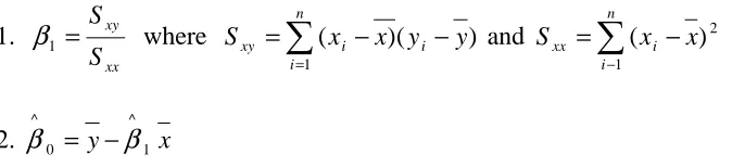
predicted values and the actual values. The least squares regression technique is based on the
Least Squares Equations seen below in Figure 2.3
1. xx xy S S = 1
β
where∑
= − − = n i i i
xy x x y y
S
1
) ( )
( and
∑
− − = n
i i
xx x x
S 1
2 ) (
2. y 1 x
^
0 ^
β
β = −
Stepwise regression is the method used to add or subtract the terms of a model in an attempt
to better explain or predict the output by creating a formula based on the input variables
and/or terms. This can be done using 1st, 2nd, 3rd, or even higher order inputs based on the
desired complexity of the model. In forward stepwise regression, terms are added based on
their ability to positively impact the model’s prediction capabilities which is known as the
significance, or p-value, of the term. The p-value is relevant to the amount of variability
attributed to that term, thus, the closer to zero, the better. Following a term being added, the
model is re-evaluated along with other potential terms to determine if any additional terms
should be added. When no further terms meet the criteria for addition to the model, the
process is terminated and that model is used as the meta-model to predict outputs based on
predetermined inputs. [Rawlings 1998].
2.4.2 Neural Network
An Artificial Neural Network, commonly referred to as a neural network, is another method
that can be used to create a meta-model and is often referred a nonlinear regression technique
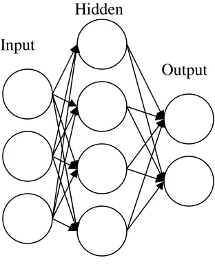
based on simulating biological neural networks. A neural network consists of nodes
(neurons); input, hidden, and output nodes. These highly interconnected nodes work together
.
Figure 2.4: Basic Neural Network
Similar to biological neural networks, artificial neural networks must be trained to solve the
problem they are modeling. There are three basic types of neural networks based on the
learning paradigms: Supervised, Unsupervised, and Reinforcement. Supervised training uses
input and corresponding output data to train the model to predict outputs from new unseen
inputs which is basically a regression technique. Therefore, the remainder of the discussion
will focus on supervised learning neural networks. In order to accomplish the modeling of a
simulation, it is necessary to have a training population based off the simulation that can be
used as a starting point to train the neural network. The accuracy of the meta-model created
in the neural network is dependent on the amount of data in the training population. Input
Hidden
2.4.3 Neural Network Training
There are multiple ways to train a neural network. A widely used method is
backpropagation. This is a gradient descent method based on minimizing the error between
the actual output of the training population and the projected output of the neural network
which is similar to the output of least squares regression method. There are two methods
that can be used to train the neural network where training refers to setting the weights of the
various nodes. The first method introduces one training set (i.e., one set of input and output
combinations) at a time which is referred to as the pattern form, while the second introduces
the entire training population or batch form (Li 2001). The backpropagation algorithm of
both methods is similar in that weights are adjusted based off the network predicted outcome
and the training set outcome.
Backpropagation Algorithm (Li 2000):
1. The training population is presented to the neural network which has random weights assigned.
2. The input variables are passed through the network and the network output (yp) is
compared against the actual output (ya) from the training set. The error is calculated
by:
∑
−= 2
) (
)
(n Ya Yp
ε
– Batch Training)) ( ) ( ( )) ( ) ( ( 2 / 1 )
(n = d n −y n τ d n −y n
ε - Pattern Form
3. Adjust the weights of the each node based on the gradient and calculated error to minimize the difference in step 2
4. Assign weights to previous layers in the same manner.
In the pattern form of backpropagation the error is calculated on an individual training point
and the weights adjusted in small increments. This is continued for each of the training points
in the training population. One cycle of the complete training population is called an epoch.
Following completion of this epoch, the data points are assigned random numbers and re-fed
through the algorithm. This is completed until a termination criterion is reached (Li 2000).
The batch form performs in a similar manner except that the error of a set of training points is
computed and the weights adjusted. The training batch does not necessarily make up the
entire training population (Li 2000).
There are many variations of the backpropagation algorithm. The simplest is the one
where the weights are adjusted in the direction that causes the greatest impact on the error
function, Gradient Descent. The amount that the weights are adjusted is constant. A
variation of this method is to increase the amount of weight change each iteration in the same
direction as long as the error function is being minimized, or a Learning Gradient Descent.
Gradient Descent Momentum allows the network to respond to the recent trends in the
gradient surface as well as the most recent gradient. This prevents the training algorithm
from getting hung-up in a local minimum [Matlab- 2009].
Other methods exist to further speed up the network training and expedite
convergence. The network used in the forthcoming experiments utilizes a scaled conjugate
gradient algorithm developed by Bishop in 1995 in his paper Network for Pattern
steepest descent path as opposed to only the steepest descent single gradient path [Matlab -
2009]. One the network has been trained it can then be used as a meta-model for the
optimization function to operate on.
The neural network used in this paper is modified from the netlab library for Matlab
based of the approach and techniques described in Neural Networks for Pattern Recognition
(Bishop 1995). The network itself consists of two layers; comprised of one input layer and
one hidden layer, feed forward network with a single output. The hidden layer consists of
ten hidden nodes with the input layer having the same number of input nodes as input
variables. Node weights prior to training are randomly assigned from the 0 mean Gaussian
distribution. The size of the training population and the termination criteria is an
experimental criterion.
2.5
Simulation Optimization – Why we need meta-models
Simulation is computationally a very expensive operation. The computational cost varies
based on the complexity of the simulation itself. Stochastic inputs will further increase this
cost due to the necessity to run multiple simulations for each input variable setting to
determine the average value of the output or confidence. That being said, optimization
methods used on the simulation itself can be extremely expensive. An optimization method
requires a large population and utilizes the computer to generate many points during each
generation. Many individuals are often poor and will die off in subsequent generations. Also
early in the search, the GA just needs to move into the general area of the optimal solution
before it fine tunes to find the actual optimal. Each new individual requires an evaluation
which in this case is a simulation model. It is apparent how the cost of these optimization
methods would be unacceptable. Therefore, it is highly desirable to utilize a less expensive
surrogate model (i.e., meta-model). The optimization function can use the meta-model for
evaluation for a portion of the time and as well as early in the cycle to reduce the amount of
true simulations needed. The goal will be to combine a simulation meta-model with the
optimization tool to create a more efficient and effective optimization technique. The goal is
to determine the best settings when using a RSM and Neural Networks as the meta-models to
assist in the determination of the optimum value in a simulation.
2.6
Approach
Specific optimization problems were chosen to represent simulation models and have been
shown to cause difficulty for deterministic optimization methods. A genetic algorithm will
be used for the optimization technique and neural networks and step-wise regression for two
potential meta-modeling techniques.
In Chapter Three, the first step will be to determine the effectiveness of each
order to evaluate this, we will conduct the experiment on two non-linear problems with
known solutions, the Brown and Schwefel problems. Initially, the two options will be tested
in a full-factorial design in a deterministic experiment. This experiment will allow the
meta-modeling techniques and optimization algorithm to operate with the distraction of noise.
Different attributes of each meta-modeling technique will be tested at various levels to
determine the effect, if any, that they have on the effectiveness of the meta-model in
determining the optimal solution. Following this experiment noise will be added to the
problem in Chapter four. This is designed to test the meta-model’s performance in a
3
Deterministic Experimental Procedure
Most simulations are stochastic in nature and therefore produce stochastic output as stated in
Chapter 2. This additional level of complexity (i.e., noisy solution values) may confound
other factors. Therefore the first experiment will eliminate the noise factor and solve several
known deterministic optimization problems utilizing meta-models which will serve two
purposes. First it will determine which factors (number of training points, response surface
methodology, etc) provide the most influence on the quality of the final solution, where the
quality of the final solution is determined by its overall value and computational efficiency.
Second, the experiment will also determine the effectiveness of linear regression and neural
networks in successfully modeling the complex functions.
The first experiment will minimize two sample problems under a different number of
variables, the Schwefel function and Brown’s almost linear function [Humphrey 2000]. The
Schwefel (Sine Root) Function Brown’s Almost Linear Function ) 1 ) sin( * ( * 8762 . 122 ( )
(X =− n+sum
∑
−x x −θ
( ) [ ( )]2 11 1 + − =
∑
= x f X f d t θ Where∑
= + − + = d j j ii x x x d
f 1 ) 1 ( )
( for
i = 1, …, d-1, and
∏
= − − d j jd x x
f 1 1 ) ( ) ( Optimal Values
Y= -1 Y= -1
Figure 3.3: Brown’s Almost Linear Function [Humphrey, 2000]
As mentioned in Chapter 2, genetic algorithms typically maximize functions. Therefore,
these minimization functions are turned into maximization problems by negating the solution
value, in effect, mirroring them around the X-axis. The sample functions were designed to
represent the non-linear nature and complexity of an actual real world problem. The initial
experiment also serves to determine whether or not the linear regression modeling technique
is capable of approximating non-linear models. The initial suspicion is that it will not yield a
high degree of approximation; however it may yield a capable method of removing some of
3.1
Experimental Setup
The ultimate goal is to develop an effective simulation optimization methodology. In order to
develop simulation optimization methodologies, researchers often imitate a true simulation
by adding noise to a known deterministic optimization problem. Therefore, the evaluation
function only takes seconds rather than minutes or hours to evaluate. The noise is frequently
nothing more than a random number generated from a known distribution, such as the
normal, with a known standard deviation. Humphrey and Wilson (2000) have shown this
technique to be a capable method of simulation optimization modeling. Again, the noise term
is omitted in the first experiment to create a deterministic evaluation function. A
deterministic evaluation function allows for a clear understanding of the effect the parameters
being tested have on explaining the variation within the experiment and their significance.
Four parameters are tested that are applicable to both the neural network and stepwise
regression meta-modeling techniques. An additional parameter that is uniquely applicable to
the stepwise regression meta-modeling technique is also evaluated within the stepwise
regression portion of the experiment. This parameter is the significance factor that is
achieved for a term to be added into the model, or the ρ-value required. The four parameters
for both modeling techniques are the size of the training population, the number of
generations the genetic algorithm searches, the amount of time the true evaluation function is
To fully understand the effect and significance that a parameter may have on the
meta-modeling technique, it is necessary to evaluate that parameter on problems of various
complexities. Therefore, the experiment has three different variable settings for each of the
two optimization functions representing various levels of complexity. A function with two
variables represents a simpler problem while ten and twenty variable functions represent
moderate to complex problems respectively.
In order maintain comparability of the different parameter values it was necessary to
begin the genetic algorithm with the same starting population for each combination of
parameter settings. This is accomplished by beginning the random number generator at a
known value, or seed which ensures that the starting population will be same for each
experimental run. Also, the common random number method is carried over to the
replication portion of the experiment with each replication beginning at a known seed. For
example, replication one begins at seed one, replication two at seed two, and so forth.
Common random numbers will be particularly useful while testing the retraining parameter.
3.1.1 Experimental Parameters
The following parameters will be evaluated on their impact on the effectiveness of the
various simulation optimization methodologies during this experimentation.
NumVar--The number of variables used to obtain the output value. This controls the relative
complexity of the problem as discussed above.
NumTrain--This represents the size of the training population. Both modeling techniques
require a population of known output values to train the meta-model. The training is done by
two different methods (i.e., Neural-Network back-propagation algorithm and least squares
linear regression) but both work by reducing the total amount of error between the predicted
value and the actual value as discussed. These actual values and predictive variables are
taken from the training population. One goal is to determine whether the size of the training
population has an effect on the final solution quality, and if so, what size provides the best
solution quality.
TermOpts—The maximum amount of generations/iterations the genetic algorithm is allowed
to search for the optimal solution. The meta-model is less complex in comparison to the
actual function that it is modeling. Theoretically, this simpler version should be easier to
solve taking the genetic algorithm less time to find the best solution. It is also an assumption
that increasing the complexity of the problems by increasing the number of variables will
TrueEval(evalOpts)--The percentage of times that the true evaluation function (i.e., the
actual simulation) is used to evaluate the individuals created by the genetic algorithm as
compared to the meta-model only. The goal of this parameter is to determine if evaluating
the true function a portion of the time affects the solution quality since the meta-model is an
approximation to the true model. It may be beneficial to access the true model periodically
to validate the values produced by the meta-model. In order to determine this point in the
evaluation function, a random number is generated and compared to the parameter value. If
it is less, then the true simulations is used to evaluate the individual otherwise the
meta-model is evaluated
Retrain--Retraining or not retraining between replications. The experiment is set up to
utilize the same meta-model for as long as possible (i.e. that the meta-model is not retrained
between replications, true evaluation parameter changes, and termination operator parameter
changes). The various parameter settings utilize the same meta-model to obtain the solution.
If retraining is used, the meta-model is retrained between every replication, creating a new
meta-model for every time. Otherwise the same meta-model is used for all replications. This
is used to determine if retraining the meta-model on a constant basis is beneficial to obtaining
a high solution quality. The goal is to determine how beneficial is when taking into account
to the computational effort needed to train a meta-model on a complex data set; one with
P-value--Represents the level of significance necessary for an explanatory variable to be
added to the model. This parameter is exclusive to the stepwise regression
meta-modeling technique. If the probability that the effect of the explanatory variable is created by
noise is less than the p-value dictated in the parameter, seen in Table 3.1: Parameters and
Settings, then the explanatory variable is added to the meta-model. In turn, this acts as a
method of excluding insignificant explanatory variables. Two parameter levels were used.
The higher level will accept more terms into the model, creating a more complex
meta-model while also increasing the probability that an insignificant explanatory variable will be
added to the model. The goal is to determine if this parameter has an effect on the final
solution quality. Table 3.1 depicts the various parameters that will be used in this experiment
along with the number of levels and their values.
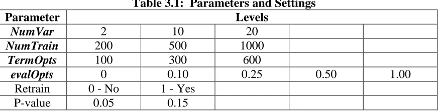
Table 3.1: Parameters and Settings
Parameter Levels
NumVar 2 10 20
NumTrain 200 500 1000
TermOpts 100 300 600
evalOpts 0 0.10 0.25 0.50 1.00
Retrain 0 - No 1 - Yes
3.1.2 Experimental Procedure Step-by-Step
The computational experiment can be subdivided into two basic procedures. The first
procedure, depicted in Figure 3.4, deals with the experiment where the meta-model is not
retrained between replications while Figure 3.5 shows the procedure where the meta-model is
1. Choose evaluation function – Schwefel or Brown 2. Choose number of variables – 2, 10, or 20
3. Set random number generator to random seed #Replication 4. Choose training sample size and create training population using
chosen evaluation function
5. Fit meta-model utilizing chosen meta-modeling technique 6. Utilize meta model to find optimum value using different values
of maximum number of generations and the amount of time the true function is used for evaluation
7. Repeat step 6 for nine additional search replications. Begin each search replication from a known random number generator seed 8. Repeat steps 1 thru 7 for each combination of function, number
of variables, and size of the training population
Figure 3.4: Step-by-Step Procedure: No Retrain
1. Choose evaluation function – Schwefel or Brown 2. Choose number of variables – 2, 10, 20
3. Choose training sample size
4. Choose maximum number of generations and evaluation options.
5. Set random number generator to known value corresponding with searching replication number.
6. Create training sample and fit model using chosen meta-modeling technique
7. Optimize using genetic algorithm
8. Repeat the step 6 for nine additional search replications. Begin each search replication from a know random number generator seed
9. Repeat steps 5 thru 7 for all combinations of variables
3.2
Experimental Design
The experimental design which utilizes the procedures in Figure 3.4 and Figure 3.5 is a five
factor, full factorial conducted on three different variable settings, two meta-modeling
techniques, and two known functions. In effect, the experiment becomes an eight factor
design. Only interaction effects for the initial five factors are observed: the number of
variables, number to train, number of generations, true evaluation ratio, and ρ-value. A tree
42
Evaluation Function –
Brown & Schwefel
Model
Neural Network Stepwise Regression
2 10 20 Number Variables 2 10 20
200 500 1000
0.05 0.15
200 500 1000
Number to Train
100 300 600
100 300 600 Number of Generations
0.10 0.25 0.50 1.00
0.00
0.10 0.25 0.50 1.00
0.00 Evaluation True
p-Val
Deterministic Experiment Setup
**Same Structure for Retrain and No Retrain
3.3
Output Data
The experimentation code is set up to record the parameter values along with a series of other
values that will determine the efficiency and the effectiveness of the combined
meta-modeling and search technique. The number of times that the meta-model is evaluated is
kept along with the number of times the true evaluation function is used to determine if there
is a relationship between those values and the final outcome. When the genetic algorithm
finds the best solution, the generation is stored to determine the efficiency of the search
technique relative to the parameter values in the experiment.
3.4
Results
Following the conclusion of the experiment, the data is collected and analyzed to determine
the significance of the parameter effects. The analysis is divided by problems, Schwefel and
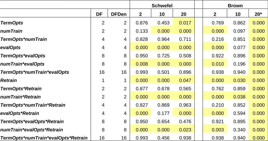
Brown, and then further divided by meta-modeling techniques. The significance values in
Table 3.2 represent the probability that the parameter effect is caused by noise. The
significance test is conducted on the maximum number of generations, the size of the training
population, and the amount of time to evaluate the true model represented as both a
continuous and a categorical variable to determine the effect that varying the modeling
technique poses on the significance level. The change in modeling type resulted in different
meta-modeling technique did not change drastically. However, the meta-modeling type change in the
regression meta-modeling technique created a significant difference in the significant terms
as seen in Table 3.6 . This shift is discussed further in Regression. Using the screening test
results from this chapter, the total number of variables can be reduced and only the terms that
are determined important have to be screed in the full model of chapter five. This produces a
reduced number of parameters that has to be statistically analyzed and compared.
3.4.1 Neural Network
Analysis of the neural network meta-modeling technique provides insight into the parameters
that hold the most significance on the final solution quality. The continuous and categorical
variable parameter modeling types produce very similar parameter significances. The
exception is the variable associated with the maximum number of generations, amount of
time the true model is evaluated, and the retraining parameter interaction as seen in Table
3.2. Due to the experimental setup it is necessary to separate the analysis into retrain and non
retrain sections. This is due to the fact that when retraining is not used the effect of the size
of the training population is not clear. It is not clear because the meta-model is only
recreated when adjusting the size of the training population. The significant effects of the
retraining portion of the experiment are presented in using the parameter names explained in
section 3.1.1. Significance levels high-lighted in yellow represent the parameters that are
found to be statistically significant. A Residual Maximum Likelihood Estimation (REML)

![Figure 3.3: Brown’s Almost Linear Function [Humphrey, 2000]](https://thumb-us.123doks.com/thumbv2/123dok_us/4490.1155069/44.612.165.460.78.284/figure-brown-s-linear-function-humphrey.webp)