Solving a mixed boundary value problem via an integral equation with the generalized neumann kernel on unbounded multiply connected region

Malaysian Journal of Fundamental & Applied Sciences

available online at

http://mjfas.ibnusina.utm.my

Solving a Mixed Boundary Value Problem via an Integral Equation with

Generalized Neumann Kernel on Unbounded Multiply Connected Region

S.A.A. Alhatemi1, A.H.M. Murid1* and M.M.S. Nasser2

1_{Department of Mathematical Sciences, Faculty of Science, Universiti Teknologi Malaysia, 81310 UTM Skudai, Johor, Malaysia .} 2_{Department of Mathematics, Faculty of Science, King Khalid University, P.O. Box 9004, Abha, Saudia Arabia.}

Received 26 November 2011, Revised 1 May 2012, Accepted 22 May 2012, Available online 15 June 2012

ABSTRACT

In this paper, we solve the mixed boundary value problem on unbounded multiply connected region by using the method of boundary integral equation. Our approach in this paper is to reformulate the mixed boundary value problem into the form of Riemann-Hilbert problem. The Riemann-Hilbert problem is then solved using a uniquely solvable Fredholm integral equation on the boundary of the region. The kernel of this integral equation is the generalized Neumann kernel. As an examination of the proposed method, some numerical examples for some different test regions are presented. | Riemann-Hilbert Problem | Integral Equation | Generalized Neumann Kernel | Laplace Equation | Mixed Boundary Value Problem |

® 2012 Ibnu Sina Institute. All rights reserved.

1. INTRODUCTION

The need to solve Laplace equation with different types of boundary conditions on different parts of a connected boundary often arises in computational physics and mechanics. Common mixed boundary conditions are mixed Dirichlet and Neumann type conditions. Recently, the interplay of Riemann-Hilbert problem and integral equation with the generalized Neumann kernel has been investigated in [1-3].

It has been shown that the problem of conformal mapping, Dirichlet problem, and Neumann problem can all be treated as Riemann Hilbert problems [2-4]. Hence they can be solved efficiently using integral equations with the generalized Neumann kernel. The boundary integral equation method is a classical method for solving the Dirichlet and Neumann boundary value problem. The classical boundary integral method for the Dirichlet problem and the Neumann problem are in the form of second kind Fredholm integral equations with the Neumann kernel. Those integral equations are derived by representing the solutions of the mixed problem as the potential of a single layer [5].

In this paper, we extend the result in [6] to solve Laplace equation on unbounded multiply connected region with Dirichlet-Neumann condition via an integral equation with the generalized Neumann kernel. This extends the

*Corresponding author at:

E-mail addresses: [email protected] (A.H.M. Murid)

results of [4]. A Fredholm integral equation of the second kind with the generalized Neumann kernel is derived for the mixed boundary value problem.

This paper is organized as follows: Section 2 presents some auxiliary materials related to the mixed problem, the Riemann-Hilbert problems as well as integral equation for Riemann-Hilbert problems. In Section 3, we reduce the mixed boundary value problem into the Riemann-Hilbert problem and construct the boundary integral equation for solving it. We will discuss the question on how to treat the integral equations numerically in Section 4. Some numerical examples are presented in Section 5. In Section 6, a short conclusion is given.

2. AUXILIARY MATERIAL

Let G be a bounded multiply connected region. The boundary

Γ

=

∂

G

consists of m Jordan curves

,

1,...,

j

j

m

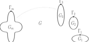
Fig. 1 Unbounded multiply connected region of connectivity m

=

)

(

s

η

⎩

⎪

⎨

⎪

⎧

1 1

2 2

( ),

[0, 2 ],

( ),

[0, 2 ],

( ),

[0, 2 ].

m m

s

s

J

s

s

J

s

s

J

η

π

η

π

η

π

∈

=

∈

=

∈

=



,

(1)

where

η

_jis twice continuously differentiable with

0

≠

ds

d

η

. The total parameter region J is the disjoint union of the intervals

J

_j

,

j

=

1

,

2

,...,

m

. Let

A

_kbe a

2

π

-periodic continuously differentiable function on

J

_kwith

0

≠

k

A

, defined on the total parameterized region

J

by

𝐴𝐴(𝑠𝑠) =

⎩ ⎪ ⎨ ⎪

⎧ 1 1

2 2

( ),

[0, 2 ],

( ),

[0, 2 ],

( ),

[0, 2].

m m

A s

s

J

A s

s

J

A s

s

J

π

π

∈ =

∈

=

∈

=



(2)

3. GENERALIZED NEUMANN KERNEL AND MIXED BOUNDARY VALUE PROBLEM

In view of the parameterization domain of the boundary

Γ

, the above formula defines also the function

A

implicitly on the boundary

Γ

. We define the reals generalized Neumann kernel N by [1-3]

𝑁𝑁

(

𝑠𝑠

,

𝑡𝑡

) =

1

_𝜋𝜋

Im

�

𝐴𝐴

_𝐴𝐴

(

₍

𝑠𝑠

_𝑡𝑡

₎

)

_𝜂𝜂

₍

_𝑡𝑡

₎

𝜂𝜂̇

_{− 𝜂𝜂}

(

𝑡𝑡

)

₍

_𝑠𝑠

₎

�

,

𝑠𝑠 ≠ 𝑡𝑡

. (3)

It is continuous at s=t with

1

1 ( )

( )

( , )

Im

.

(4)

2 ( )

( )

t

A t

N t t

t

A t

η

π

η





=

_

−

_











We define the real kernel

M

as

𝑀𝑀

(

𝑠𝑠

,

𝑡𝑡

) =

1

_𝜋𝜋

Re

�

𝐴𝐴

_𝐴𝐴

(

₍

𝑠𝑠

_𝑡𝑡

₎

)

_𝜂𝜂

₍

_𝑡𝑡

₎

𝜂𝜂̇

_{− 𝜂𝜂}

(

𝑡𝑡

)

₍

_𝑠𝑠

₎

�

,

𝑠𝑠 ≠ 𝑡𝑡

. (5)

When

s

,

t

∈

J

_kin the same parameter interval

J

_k

,

𝑀𝑀(𝑠𝑠,𝑡𝑡) =₂1_𝜋𝜋

cot

�𝑠𝑠 − 𝑡𝑡₂ �+𝑀𝑀1(𝑠𝑠,𝑡𝑡), 𝑠𝑠,𝑡𝑡 ∈ 𝐽𝐽𝑘𝑘. (6)

with a continuous kernel

M

₁ which take on the diagonal the values

𝑀𝑀

(

t

,

t

)

=1

𝜋𝜋 ℜ � 1 2 𝜂𝜂̈(𝑡𝑡) 𝜂𝜂̇(𝑡𝑡)− 𝐴𝐴̇(𝑡𝑡)

𝐴𝐴(𝑡𝑡)�, 𝑠𝑠=𝑡𝑡. (7)

Define the integral operators

) 9 ( , ) ( ) , ( ) )( ( ) 8 ( , ) ( ) , ( ) )( (

∫

∫

= = J J dt t t s M s dt t t s N s

µ

µ

µ

µ

M N

where the integral in (9) is a principal value integral.

The solvability of boundary integral equations with the generalized Neumann kernel is determined by the index (winding number in other terminology) of the function 𝐴𝐴 [1,5,6].

For the function 𝐴𝐴given by

𝐴𝐴(𝑠𝑠) =

⎩ ⎪ ⎨ ⎪

⎧_𝑐𝑐 𝑐𝑐1, 𝑠𝑠 ∈ 𝐽𝐽1= [0,2𝜋𝜋], 2, 𝑠𝑠 ∈ 𝐽𝐽2= [0,2𝜋𝜋],

⋮ ⋮

𝑐𝑐𝑚𝑚, 𝑠𝑠 ∈ 𝐽𝐽𝑚𝑚 = [0,2𝜋𝜋],

where c_j are complex constants, the index 𝜅𝜅_𝑗𝑗,𝑗𝑗= 1,2, … ,𝑚𝑚 of 𝐴𝐴 on the curve Γ_𝑗𝑗 ,𝑗𝑗= 1,2, … ,𝑚𝑚 and the indexes

𝜅𝜅=� 𝜅𝜅𝑗𝑗 𝑚𝑚

𝑗𝑗=1

,

of 𝐴𝐴 of the whole boundary are given by

𝜅𝜅𝐽𝐽 = 0, 𝜅𝜅= 0.

Let 𝐻𝐻 be the space of all continuous H𝑜𝑜̈lder functions on the boundary Γ and let 𝑆𝑆 be the subspace of 𝐻𝐻which consists of all piecewise constant functions defined on Γ. Thus, we have from [1,2,7] the following theorem.

Theorem 2.1. For a function 𝛾𝛾 ∈ 𝐻𝐻, there exist unique

functions ℎ ∈ 𝑆𝑆 and 𝜇𝜇 ∈ 𝐻𝐻 such that

are boundary values of unique function 𝐴𝐴(𝑧𝑧)in 𝐺𝐺 with 𝐴𝐴(∞) = 0 for unbounded 𝐺𝐺, where 𝜇𝜇 is a unique solution of the integral equation

𝜇𝜇 − 𝑵𝑵𝜇𝜇=−𝑴𝑴𝛾𝛾,

and the function h is given by

ℎ= [𝑴𝑴𝜇𝜇 −(𝑰𝑰 − 𝑵𝑵)𝛾𝛾]/2.

4. REDUCTION OF MIXED BOUNDARY VALUE PROBLEM TO RIEMANN -HILBERT PROBLEM.

In this section we show how to reduce the mixed boundary problem into the form of Riemann-Hilbert problem on multiply connected region.

Let 𝒏𝒏be the exterior normal to Γ and let 𝜙𝜙 ∈ 𝐻𝐻 be a given function. However, the function

𝐹𝐹

(

𝑧𝑧

)

is in general a multi-valued function.

Without lost of generality, we consider solving Laplace equation with Dirichlet condition on

Γ

₁

,



,

Γ

_l and Neumann condition on

Γ

_l+₁

,



,

Γ

_m. We shall

consider the mixed boundary value problem. Define a real function 𝑢𝑢 such that

Δ𝑢𝑢= 0 𝑎𝑎 in 𝐺𝐺,

𝑢𝑢=𝜙𝜙𝑗𝑗on Γj, j = 1, … ,𝑙𝑙, 𝜕𝜕𝑢𝑢

𝜕𝜕𝒏𝒏=𝜙𝜙𝑗𝑗on Γj, j =𝑙𝑙+ 1, … . , m

The unique solution

u

(

z

)

of the mixed boundary value problem can be regarded as a real part of an analytic function

𝐹𝐹

(

𝑧𝑧

) =

𝑢𝑢

(

𝑧𝑧

) +

𝑖𝑖

𝑣𝑣

(

𝑧𝑧

)

. We define a complex-valued [8,9] function

𝐴𝐴̂

(

𝑠𝑠

)

and a real-valued function

𝛾𝛾

(

𝑠𝑠

)

for

𝑠𝑠 ∈ 𝐽𝐽

_𝑗𝑗,

𝑗𝑗

= 1, … ,

𝑙𝑙

, by

𝐴𝐴̂

𝑗𝑗

(

𝑠𝑠

) = 1,

𝛾𝛾

𝑗𝑗

(

𝑠𝑠

) =

𝜙𝜙

𝑗𝑗

(

𝑠𝑠

),

and using the Cauchy-Riemann equations for

𝑠𝑠 ∈ 𝐽𝐽

_𝑗𝑗,

𝑗𝑗

=

𝑙𝑙

+ 1, … ,

𝑚𝑚

, by

𝐴𝐴̂

𝑗𝑗

(

𝑠𝑠

) =

−𝑖𝑖

,

𝛾𝛾

𝑗𝑗

(

𝑠𝑠

) =

� 𝜙𝜙

𝑗𝑗

(

𝑡𝑡

)

�𝜂𝜂̇

𝑗𝑗

(

𝑡𝑡

)

�𝑑𝑑𝑡𝑡

𝑠𝑠

0

.

Let also

ℎ�

(

𝑠𝑠

)

be the piecewise constant function

ℎ�(𝑠𝑠) =�_𝑐𝑐0, 𝑠𝑠 ∈ 𝐽𝐽𝑗𝑗 = [0,2𝜋𝜋], 𝑗𝑗= 1, … ,𝑙𝑙

𝑗𝑗, 𝑠𝑠 ∈ 𝐽𝐽𝑗𝑗 = [0,2𝜋𝜋], 𝑗𝑗=𝑙𝑙+ 1, … ,𝑚𝑚

where

𝑐𝑐

_𝑗𝑗,

𝑗𝑗

=

𝑙𝑙

+ 1, … ,

𝑚𝑚

, are undetermined real constants. Thus the boundary values of the function

𝐹𝐹

(

𝑧𝑧

)

satisfy the boundary condition [2-4]

Re

�𝐴𝐴̂

(

𝑠𝑠

)

𝐹𝐹

(

𝑠𝑠

)

�

=

𝛾𝛾

(

𝑠𝑠

) +

ℎ�

(

𝑠𝑠

) ,

𝑠𝑠 ∈ 𝐽𝐽

.

The function

F

(

z

)

can be written as

),

log(

)

(

ˆ

)

(

1

j m

j

j

z

z

a

z

F

z

F

=

−

∑

−

=

where

F

ˆ

(

z

)

is a single-valued analytic function in

G

,

z

_j

is a fixed point in

G

and

a

_j is undetermined real constant,

j

=

1

,

2

,...,

m

[4,10]. We assume that the

function

F

ˆ

(

z

)

satisfies

ℑ

F

ˆ

(

∞

)

=

0

in

G

.

In this paper we shall consider only the case for which

,

0

=

j

a

j

=

1

,

2

,...,

m

Thus the function

F

ˆ

(

z

)

is a solution of the Riemann-Hilbert problem

Re

�𝐴𝐴̂

(

𝑠𝑠

)

𝐹𝐹�

(

𝑠𝑠

)

�

=

𝛾𝛾

(

𝑠𝑠

) +

ℎ�

(

𝑠𝑠

) ,

𝑠𝑠 ∈ 𝐽𝐽

. (10)

Let

𝐹𝐹�

(

∞

) =

𝑐𝑐̂

(real constant), then the function

𝑔𝑔

(

𝑧𝑧

) =

𝐹𝐹�

(

𝑧𝑧

)

− 𝑐𝑐̂

is analytic single-valued function in G. Thus

𝐴𝐴̂

(

𝑠𝑠

)

𝐹𝐹��𝜂𝜂

(

𝑠𝑠

)

�

=

𝐴𝐴̂

(

𝑠𝑠

)

𝑔𝑔�𝜂𝜂

(

𝑠𝑠

)

�

+

𝐴𝐴̂

(

𝑠𝑠

)

𝑐𝑐̂

.

Hence (10) can be written as

Re[

𝐴𝐴

(

𝑠𝑠

)

𝑔𝑔

(

𝜂𝜂

(

𝑠𝑠

))] =

𝛾𝛾

(

𝑠𝑠

) +

ℎ

(

𝑠𝑠

)

,

where

𝐴𝐴

(

𝑠𝑠

) =

𝐴𝐴̂

(

𝑠𝑠

),

ℎ

(

𝑠𝑠

) =

ℎ�

(

𝑠𝑠

)

− 𝑅𝑅𝑅𝑅

[

𝐴𝐴̂

(

𝑠𝑠

)

𝑐𝑐

�

]

.

According to Theorem 1, let

µ

=

Im

Ag

(unknown function), then

)

(

)

(

)

(

)

(

)

(

s

g

s

s

h

s

i

s

A

=

γ

+

+

µ

where

µ

is the unique solution of the integral equation

γ

µ

µ

−

N

=

−

M

, (11)

𝑤𝑤

here N and M are defined as in(8) and (9). By obtaining

𝜇𝜇

, we can get

ℎ

from

2

/

]

)

(

[

M

µ

I

N

γ

h

=

−

−

.

5. NUMERICAL IMPLEMENTATIONS

Since the functions 𝐴𝐴_𝑗𝑗 and 𝜂𝜂_𝑗𝑗are 2𝜋𝜋-periodic, the integrals in the operators N and M in the integral equation (11) can be best discretized on an equidistant grid by the trapezoidal rule [5]. The computational details are similar to previous works [6].

By using the trapezoidal rule with n (an even positive integer) equidistant collocation points on each boundary component, solving the integral equations (11) reduces to solving mn by mn linear systems. Since the integral equations (11) are uniquely solvable, then for sufficiently large values of n the obtained linear systems are also uniquely solvable[1].

In this paper, the linear systems are solved using the Gauss elimination method. By solving the linear systems, we obtain approximations to 𝜇𝜇. Hence, we obtain approximations to ℎ�. Then, we obtain approximation to the constants c, and c_j for j= l+1,…,m. Hence, we obtain approximations to the boundary values of the function g(z) from

Ag

=

γ

+

h

+

i

µ

. Then the values of g(z) for z∈ G will be calculated by the Cauchy integral formula. For pointsz which are not close to the boundaryΓ, the integrals in the Cauchy integral formula are approximated by the trapezoidal rule. However, for points z near the boundary Γ, the integrand is nearly singular. For the latter case, the integral in the Cauchy integral formula can be calculated accurately using the method suggested.

6. NUMERICAL EXAMPLES

To illustrate this approach, we consider three test regions. By |u(z)−

u

_n(z)|where un(z) is the numerical

approximation of u(z).The result can be shown in Table1,Table2,Table3.

6.1 Example 1

In this example we consider a unbounded multiply connected region of connectivity 3 unbounded by the three circles

it

e

−

+

=

Γ

₁

:

η

₁

1

0

.

5

,

it

e

−

−

=

Γ

₂

:

η

₂

1

0

.

5

,

3 3

:

η

Γ

=

0

.

2

e

−it

We assume that the condition on the boundaries Γ₁,Γ₂ is the Neumann condition and the condition on the

boundaries Γ₃ is the Dirichlet condition. In this example we used the exact solution

ℜ(𝐹𝐹) =ℜ �1_𝑧𝑧�.

To obtain 𝜙𝜙_1,2for the Neumann condition we differentiate with respect to the normal the real part of the exact solution.

Fig. 2 The unbounded multiply regions of 3-circles connectivities

Table 1 The error norm|u(z)−

u

_n(z)|

n Z=0.3 Z=0.9i Z=-0.7 Z=-0.3i 16 1(-03) 5(-7) 2(-6) 2(-7) 32 5(-10) 8(-19) 5(-09) 3(-16)

64 2(-16) 9(-19) 3(-17) 5(-21)

6.2 Example

In this example we consider a unbounded multiply connected region of connectivity 4 unbounded by the forth circles

it

e

−

=

Γ

₁

:

η

₁

it

e

−

+

=

Γ

2

:

η

2

5

,

5

:

3 3

it

e

=

+

−

=

Γ

η

We assume that the condition on the boundaries Γ₁,Γ₂ is the Neumann condition and the condition on the boundaries Γ₃ is the Dirichlet condition.In this example we used the exact solution

ℜ(𝐹𝐹) =ℜ �1_𝑧𝑧�.

To obtain 𝜙𝜙_1,2for the Neumann condition we integrand the real part of the exact solution.

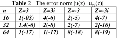
Table 2 The error norm |u(z)−

u

_n(z)|

6.3 Example 3

In this example we consider a unbounded multiply connected region of connectivity 4 unbounded by the fourth circles

it

e

i

+

−

+

=

Γ

₁

:

η

₁

3

2

it

e

i

+

−

+

−

=

Γ

₂

:

η

₂

3

2

it

e

i

+

−

+

=

Γ

3

:

η

1

3

2

:

4

Γ

it

e

i

+

−

−

=

3

2

4

η

We assume that the condition on the boundaries Γ₁,Γ₂ is the Neumann condition and the condition on the boundaries Γ₃

,

Γ

₄ is the Dirichlet condition.In this example we used the exact solution

ℜ(𝐹𝐹) =ℜ �_𝑧𝑧+3+21 _𝑖𝑖�.

To obtain 𝜙𝜙_1,2for the Neumann condition we differentiate with respect to the normal the real part of the exact solution.

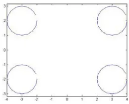
Fig. 3 The unbounded multiply regions of 4 circles connectivities

Table 3 The error norm |u(z)−

u

_n(z)|

n Z=-3 Z=1+i Z=-0.3 Z=0.3i 16 4(-6) 3(-5) 3.2(-5) 3(-05) 32 1.5(-10) 1(-10) 1.7(-10) 1(-11)

64 3.8(-16) 1(-16) 1.3(-16) 8(-17)

7. CONCLUSION

The uniquely solvable integral equation is derived in this work for the mixed boundary value problem with Dirichlet-Neumann condition on unbounded multiply connected region. The derived boundary integral equation is uniquely solvable and yields directly the boundary value of the solution of the mixed problem.

Mixed boundary value problem is solved numerically on unbounded multiply connected region using the proposed method. The numerical examples illustrate that the proposed method yields approximations of high accuracy.

ACKNOWLEDGEMENT

The authors acknowledge the financial support for this research by the Malaysian Ministry of Higher Education (MOHE) through UTM GUP Vote Q.J130000.7126.01H75 and Ibnu Sina Institute, Universiti Teknologi Malaysia, Johor for facilities.

REFERENCES

[1] M.M.S. Nasser, SIAM J. Sci. Compu. 31(2009)1695-1715. [2] R. Wegmann and M.M.S. Nasser, J. Comput. Appl. Math.

214(2008)36-57.

[3] M.M.S. Nasser, Compu. Meth. Func. Theo. 9(2009)127(143). [4] M.M.S. Nasser, A.H.M. Murid, M. Ismail & E.M.A. Alejaily, Appl.

Math. Compu. 217(2011)4710-4727.

[5] F.D. Gakhov. Boundary value problem, English translation of Russian edition 1963. Oxford Pergamon Press, 1966.

[6] S.A.A. Alhatemi, A.H.M. Murid ,M.M.S. Nasser, Proceedings in ISASM 2011, UTHM, KL, 1-3 NOV. 2011. 74-80.

[9] M.M.S. Nasser, J. Math. Anal. Appl. 382(2011)47-56.

[8] R. Haas and H. Brauchli, Comput. Meth. Appl. Mech. Engin. Vol 89, 1–3, 1991, 543–556.

[9] R. Haas and H. Brauchli, J. Comput. Appl. Math 44(1992)167-185. [10] S.G. Mikhlin, Integral Equation and their applications to certain

problems in mechanics, mathematical physics and technology, Pergamon, Armstrong, 1957.