An inverse problem statistical methodology summary

(1)

An Inverse Problem Statistical Methodology Summary

H.T. Banks, M. Davidian, J.R. Samuels, Jr. and Karyn L.Sutton

Center for Research in Scientific Computation

and

Center for Quantitative Sciences in Biomedicine

North Carolina State University

Raleigh, NC 27695-8205

and

Department of Mathematics & Statistics

Arizona State University

Tempe, AZ, 85287-1804

January 12, 2008

Abstract

We discuss statistical and computational aspects of inverse or parameter estima-tion problems based on Ordinary Least Squares and Generalized Least Squares with appropriate corresponding data noise assumptions of constant variance and noncon-stant variance (relative error), respectively. Among the topics included here are math-ematical model, statistical model and data assumptions, and some techniques (residual plots, sensitivity analysis, model comparison tests) for verifying these. The ideas are illustrated throughout with the popular logistic growth model of Verhulst and Pearl as well as with a recently developed population level model of pneumococcal disease spread.

Keywords: Inference, least squares inverse problems, parameter estimation, sensi-tivity and generalized sensisensi-tivity functions.

1

Introduction

In this Chapter we discuss mathematical and statistical aspects of inverse or parameter

estimation problems. While we briefly discuss maximum likelihood estimators (MLE), our

focus here will be onordinary least squares(OLS) andgeneralized least squares(GLS)

(2)

general nonlinear ordinary differential equation mathematical model to discuss concepts and ideas, the discussions are also applicable to partial differential equation models and other

deterministic dynamical systems. As we shall explain, the choice of an appropriate

statisti-cal model is of critical importance, and we discuss at length the difference between constant

variance and nonconstant variance noise in the observation process, the consequences for incorrect choices in this regard, and computational techniques for investigating whether a good decision has been made. In particular, we illustrate use of residual plots to suggest whether or not a correct statistical model has been specified in an inverse problem formu-lation. We illustrate these and other techniques with examples including the well known Verhulst-Pearl logistic population model and a specific epidemiological model (a pneumo-coccal disease dynamics model). We discuss the use of sensitivity equations coupled with the asymptotic theory for sampling distributions and the computation of associated covariances, standard errors and confidence intervals for the estimators of model parameters. We also

discuss sensitivity functions(traditional andgeneralized) and their emerging use in design of

experiments for data specific to models and mechanism investigation. Traditional sensitivity involves sensitivity of outputs to parameters while the recent concept of generalized sensi-tivity in inverse problems pertains to sensisensi-tivity of parameters (to be estimated) to data or observations. That is, generalized sensitivity quantifies the relevance of data measurements for identification of parameters in a typical parameter estimation problem. In a final section we present and illustrate some methods for model comparison.

2

Parameter Estimation: MLE, OLS, and GLS

2.1

The Underlying Mathematical and Statistical Models

We consider inverse or parameter estimation problems in the context of a parameterized

(with vector parameter ~θ) dynamical system ormathematical model

d~x

dt(t) =~g(t, ~x(t), ~θ) (1)

with observation process

~y(t) =C~x(t;~θ). (2)

Following usual convention (which agrees with the data usually available from experiments),

we assume a discrete form of the observations in which one hasn longitudinal observations

corresponding to

~y(tj) =C~x(tj;~θ), j = 1, . . . , n. (3)

In general the corresponding observations or data _{~y_j} will not be exactly ~y(tj). Because of

(3)

2.2

Description of Statistical Model

In our discussions here we consider a statistical model of the form

~

Yj =f~(tj, ~θ0) +~ǫj, j = 1, . . . , n, (4)

where f~(tj, ~θ) = C~x(tj;~θ), j = 1, . . . , n, corresponds to the solution of the mathematical

model (1) at the jth _{covariate for a particular vector of parameters}~θ_∈_Rp_{, ~x}_∈_RN_{, ~}_f _∈_Rm_,

and _C is an m _×N matrix. The term ~θ0 represents the “truth” or the parameters that

generate the observations {Y~j}n

j=1. (The existence of a truth parameter ~θ0 is standard in

statistical formulations and this along with the assumption that the means E[~ǫj] are zero

yields implicitly that the (1) is a correct description of the process being modeled.) The terms

~ǫj are random variables which can represent measurement error, “system fluctuations” or

other phenomena that cause observations to not fall exactly on the points f~(tj, ~θ) from the

smooth pathf~(t, ~θ). Since these fluctuations are unknown to the modeler, we will assume~ǫj

is generated from a probability distribution (with mean zero throughout our discussions) that reflects the assumptions regarding these phenomena. For instance, in a statistical model for

pharmacokinetics of drug in human blood samples, a natural distribution for~ǫ= (ǫ1, . . . , ǫn)T

might be a multivariate normal distribution. In other applications the distribution for~ǫmight

be much more complicated [22].

The purpose of our presentation here is to discuss methodology related to the

estima-tion of the true value of the parameters ~θ0 from a set Θ of admissible parameters, and its

dependence on what is assumed about the variance var(~ǫj) of the error~ǫj. We discuss two

inverse problem methodologies that can be used to calculate estimates ˆθfor ~θ0: the ordinary

least-squares (OLS) and generalized least-squares (GLS) formulations as well as the popular maximum likelihood estimate (MLE) formulation in the case one assumes the distributions

of the error process _{~ǫj} are known.

2.3

Known error processes: Normally distributed error

In the introduction of the statistical model we initially made no mention of the probability

distribution that generates the error ~ǫj. In many situations one readily assumes that the

errors ~ǫj = 1, . . . , n, are independent and identically distributed (we make the standing

assumptions of independence across j throughout our discussions in this Chapter). We

discuss a case where one is able to make further assumptions on the error, namely that the distribution is known. In this case, maximum likelihood techniques may be used. We

discuss first one such case for a scalar observation system, i.e., m= 1. If, in addition, there

is sufficient evidence to suspect the error is generated by a normal distribution then we may

be willing to assume ǫj ∼ N(0, σ02), and hence Yj ∼ N(f(tj, ~θ0), σ20). We can then obtain an

(4)

the likelihood function for ǫj =Yj−f(tj, ~θ) which is defined by

L(~θ, σ2_|_Y_~_{) =}

n

Y

j=1 1

√

2πσ2 exp{−

1

2σ2[Yj−f(tj, ~θ)]

2_}_. ₍₅₎

The resulting solutionsθMLEandσ2

MLEare the maximum likelihoodestimators(MLEs) for~θ0

andσ2

0, respectively. We point out that these solutions θMLE=θMLEn (Y~) andσ

2

MLE =σ

2n

MLE(Y~)

are random variables by virtue of the fact that Y~ is a random variable. The corresponding

maximum likelihood estimates are obtained by maximizing (5) with Y~ = (Y1, . . . , Yn)T

replaced by a given realization ~y = (y1, . . . , yn)T and will be denoted by ˆθMLE = ˆθnMLE and

ˆ

σMLE = ˆσn

MLErespectively. In our discussions here and below, almost every quantity of interest

is dependent on n, the size of the set of observations or the sampling size. On occasion we

will express this dependence explicitly by use of superscripts or subscripts, especially when we wish to remind the reader of this dependence. However, for notational convenience we

will often suppress the notation of explicit dependence on n.

Maximizing (5) is equivalent to maximizing the log likelihood

logL(~θ, σ2_|_Y_~_{) =} ₋n

2 log(2π)−

n

2logσ

2₋ 1 2σ2

n

X

j=1

[Yj−f(tj, ~θ)]2. (6)

We determine the maximum of (6) by differentiating with respect to~θ (with σ2 _{fixed) and}

with respect to σ2 _(with ~θ _{fixed), setting the resulting equations equal to zero and solving}

for ~θ and σ2_{. With} _σ2 _{fixed we solve} ∂

∂~θlogL(~θ, σ

2_|_Y_~_{) = 0 which is equivalent to}

n

X

j=1

[Yj−f(tj, ~θ)]∇f(tj, ~θ) = 0, (7)

where as usual ∇f = ∂

∂~θf = f~θ. We see that solving (7) is the same as the least squares

optimization

θMLE(Y~) = arg min

~ θ∈Θ

J(Y , ~θ~ ) = arg min

~ θ∈Θ

n

X

j=1

[Yj −f(tj, ~θ)]2. (8)

We next fix~θ to beθMLE and solve _∂σ∂2 logL(θMLE, σ2|Y~) = 0, which yields

σMLE2 (Y~) =

1

nJ(Y , θMLE~ ). (9)

Note that we can solve for θMLE and σ2

MLE separately – a desirable feature, but one that does

not arise in more complicated formulations discussed below. The 2nd _{derivative test (which}

is omitted here) verifies that the expressions above for θMLE and σ2

MLE do indeed maximize

(5)

If, however, we have a vector of observations for the jth _covariate _t

j then the statistical

model is reformulated as

~

Yj =f~(tj, ~θ0) +~ǫj (10)

where f~∈Rm _and

V0 = var(~ǫj) = diag(σ02,1, . . . , σ20,m) (11)

for j = 1, . . . , n. In this setting we have allowed for the possibility that the observation

coordinatesYi

j may have different constant variances σ02,i, i.e., σ02,i does not necessarily have

to equal σ2

0,k. If (again) there is sufficient evidence to claim the errors are independent and

identically distributed and generated by a normal distribution thenǫ~j ∼ Nm(0, V0). We thus

can obtain the maximum likelihood estimatorsθMLE({Y~j}) and VMLE({Y~j}) for θ0 and V0 by

determining the maximum of the log of the likelihood function for~ǫj =Y~j−f~(tj, ~θ) defined

by

logL(~θ, V_|{Y_j1, . . . , Y_jm_}) = ₋n 2

m

X

i=1

logσ₀2_,i₋ 1

2

m

X

i=1 1

σ2 0,i

n

X

j=1

[Y_ji₋fi(tj, ~θ)]2

=₋n

2

m

X

i=1 logσ2

0,i− n

X

j=1

[Y~j −f~(tj, ~θ)]TV

−₁

[Y~j −f~(tj, ~θ)].

Using arguments similar to those given for the scalar case, we determine the maximum

likelihood estimators for ~θ0 and V0 to be

θMLE = arg min

~ θ∈Θ

n

X

j=1

[Y~j −f~(tj, ~θ)]TVMLE−1[Y~j −f~(tj, ~θ)] (12)

VMLE = diag 1

n

X

j=1

[Y~j−f~(tj, θMLE)][Y~j −f~(tj, θMLE)]T

!

. (13)

Unfortunately, this is a coupled system, which requires some care when solving numerically. We will discuss this issue further in Sections 2.4.2 and 2.4.5 below.

2.4

Unspecified Error Distributions and Asymptotic Theory

In Section 2.3 we examined the estimates of ~θ0 and V0 under the assumption that the error

is normally distributed, independent and constant longitudinally. But what if it is suspected

that the error is not normally distributed, or the error distribution is unknown to the modeler

beyond the assumptions on E[Y~j] embodied in the model and the assumptions made on

var(~ǫj) (as in most applications)? How should we proceed in estimating ~θ0 and σ0 (or V0)

(6)

2.4.1 Ordinary Least Squares (OLS)

The statistical model in the scalar case takes the form

Yj =f(tj, ~θ0) +ǫj (14)

where the variance var(ǫj) = σ02 is assumed constant in longitudinal data (note that the

error’s distribution is not specified). We also note that the assumption that the observation

errors are uncorrelated across j (i.e., time) may be a reasonable one when the observations

are taken with sufficient intermittency or when the primary source of error is measurement error. If we define

θOLS(Y~) =θOLSn (Y~) = arg min

~ θ∈Θ

n

X

j=1

[Yj −f(tj, ~θ)]2 (15)

then θOLS can be viewed as minimizing the distance between the data and model where all

observations are treated as of equal importance. We note that minimizing in (15) corresponds

to solving for ~θin

n

X

j=1

[Yj −f(tj, ~θ)]∇f(tj, ~θ) = 0. (16)

We point out that θOLS is a random variable (ǫj =Yj−f(tj, ~θ) is a random variable); hence

if _{yj}nj=1 is a realization of the random process {Yj}nj=1 then solving

ˆ

θOLS = ˆθOLSn = arg min

~ θ∈Θ

n

X

j=1

[yj−f(tj, ~θ)]2 (17)

provides a realization for θOLS. (A remark on notation: for a random variable or estimatorθ

we will always denote a corresponding realization or estimate with an over hat, e.g., ˆθ is an

estimate for θ.)

Noting that

σ₀2 = 1

nE[

n

X

j=1

[Yj −f(tj, ~θ0)]2] (18)

suggests that once we have solved for θOLS in (15), we may obtain an estimate ˆσ2

OLS = ˆσ

2n

MLE

for σ2 0.

Even though the error’s distribution is not specified we can use asymptotic theory to

approximate the mean and variance of the random variable θOLS [31]. As will be explained

in more detail below, as n→ ∞, we have that

θOLS =θOLSn ∼ Np(~θ0,Σ

n

0)≈ Np(~θ0, σ20[χnT(~θ0)χn(~θ0)]

−₁

(7)

where the sensitivity matrix χ(~θ) =χn₍~θ_{) =}_{_χn

jk} is defined as

χn_jk(~θ) = ∂f(tj, ~θ)

∂~θk

, j = 1, . . . , n, k= 1, . . . , p,

and

Σn0 ≡σ20[nΩ0]

−₁

(20)

with

Ω0 _≡ lim

n→∞ 1

nχ

nT₍_~θ₀₎_χn₍_~θ₀₎_, ₍₂₁₎

where the limit is assumed to exist–see [31]. However,~θ0 and σ20 are generally unknown, so

one usually will instead use the realization ~y = (y1, . . . , yn)T of the random process Y~ to

obtain the estimate

ˆ

θOLS = arg min

~ θ∈Θ

n

X

j=1

[yj −f(tj, ~θ)]2 (22)

and thebias adjustedestimate

ˆ

σOLS2 =

1

n₋p

n

X

j=1

[yj−f(tj,θˆ)]2 (23)

to use as an approximation in (19).

We note that (23) represents the estimate for σ2

0 of (18) with the factor 1n replaced by

the factor 1

n−p (in the linear case the estimate with

1

n can be shown to be biased downward

and the same behavior can be observed in the general nonlinear case– see Chap. 12 of [31] and p. 28 of [22]). We remark that (18) is true even in the general nonlinear case (it does not rely on any asymptotic theories although it does depend on the assumption of constant variance being correct).

Both ˆθ = ˆθOLS and ˆσ2 _{= ˆ}_σ2

OLS will then be used to approximate the covariance matrix

Σn₀ _≈Σˆn _≡ˆσ2[χnT(ˆθ)χn(ˆθ)]−1_. ₍₂₄₎

We can obtain the standard errorsSE(ˆθOLS,k) (discussed in more detail in the next section) for

the kth _{element of ˆ}_θOLS _{by calculating} _SE_(ˆ_θOLS

,k)≈

q

ˆ

Σn

kk. Also note the similarity between

the MLE equations (8) and (9), and the scalar OLS equations (22) and (23). That is, under a normality assumption for the error, the MLE and OLS formulations are equivalent.

If, however, we have a vector of observations for the jth _covariate _t

j and we assume the

variance is still constant in longitudinal data, then the statistical model is reformulated as

~

(8)

where f~∈Rm _and

V0 = var(~ǫj) = diag(σ02,1, . . . , σ20,m) (26)

for j = 1, . . . , n. Just as in the MLE case we have allowed for the possibility that the

observation coordinates Yi

j may have different constant variances σ02,i, i.e. σ02,i does not

necessarily have to equalσ2

0,k. We note that this formulation also can be used to treat the

case where V0 is used to simply scale the observations, i.e., V0 = diag(v1, . . . , vm) is known.

In this case the formulation is simply avector OLS (sometimes also called a weighted least

squares (WLS)). The problem will consist of finding the minimizer

θOLS = arg min

~ θ∈Θ

n

X

j=1

[Y~j −f~(tj, ~θ)]TV0−1[Y~j −f~(tj, ~θ)], (27)

where the procedure weights elements of the vector Y~j−f~(tj, ~θ) according to their variability.

(Some authors refer to (27) as a generalized least squares (GLS) procedure, but we will make use of this terminology in a different formulation in subsequent discussions). Just as in the

scalar OLS case, θOLS is a random variable (again because ~ǫj = Y~j −f~(tj, ~θ) is); hence if

{~yj}nj=1 is a realization of the random process {Y~j}nj=1 then solving

ˆ

θOLS = arg min

~ θ∈Θ

n

X

j=1

[~yj−f~(tj, ~θ)]TV0−1[~yj −f~(tj, ~θ)] (28)

provides an estimate (realization) ˆθ = ˆθOLS for θOLS. By the definition of variance

V0 = diagE

1

n

X

j=1

[Y~j −f~(tj, ~θ0)][Y~j−f~(tj, ~θ0)]T

!

,

so an unbiased estimate of V0 for the realization {~yj}nj=1 is

ˆ

V = diag 1

n−p

n

X

j=1

[~yj−f~(tj,θˆ)][~yj −f~(tj,θˆ)]T

!

. (29)

However, the estimate ˆθ requires the (generally unknown) matrix V0 and V0 requires the

unknown vector ~θ0 so we will instead use the following expressions to calculate ˆθ and ˆV:

~θ0 ≈θˆ= arg min

~ θ∈Θ

n

X

j=1

[~yj −f~(tj, ~θ)]TVˆ−1[~yj−f~(tj, ~θ)] (30)

V0 ≈Vˆ = diag

1

n₋p

n

X

j=1

!

(9)

Note that the expressions for ˆθ and ˆV constitute a coupled system of equations, which will require greater effort in implementing a numerical scheme.

Just as in the scalar case we can determine the asymptotic properties of the OLS estimator

(27). As n → ∞,θOLS has the following asymptotic properties [22, 31]:

θOLS ∼ N(~θ0,Σn0), (32) where

Σn₀ ≈

n

X

j=1

D_jT(~θ0)V

−₁

0 Dj(~θ0)

!−1

, (33)

and the m×p matrix Dj(~θ) =Dnj(~θ) is given by

   

∂f1(tj,~θ)

∂θ1

∂f1(tj,~θ)

∂θ2 · · ·

∂f1(tj,~θ)

∂θp

... ... ...

∂fm(tj,~θ)

∂θ1

∂fm(tj,~θ)

∂θ2 · · ·

∂fm(tj,~θ)

∂θp     .

Since the true value of the parameters ~θ0 and V0 are unknown their estimates ˆθ and ˆV will

be used to approximate the asymptotic properties of the least squares estimator θOLS:

θOLS _{∼ N}p(~θ0,Σn0)≈ Np(ˆθ,Σˆn) (34)

where

Σn₀ _≈Σˆn =

n

X

j=1

D_jT(ˆθ) ˆV−1_D

j(ˆθ)

!−1

. (35)

The standard errors can then be calculated for the kth _{element of ˆ}_θOLS ₍_SE_(ˆ_θOLS

,k)) by

SE(ˆθOLS,k) ≈

p

ˆ

Σkk. Again, we point out the similarity between the MLE equations (12)

and (13), and the OLS equations (30) and (31) for the vector statistical model (25).

2.4.2 Numerical Implementation of the OLS Procedure

In the scalar statistical model (14), the estimates ˆθ and ˆσ can be solved for separately (this

is also true of the vector OLS in the case V0 =σ02Im, where Im is the m×m identity) and

thus the numerical implementation is straightforward - first determine ˆθOLS according to (22)

and then calculate ˆσ2

OLS according to (23). The estimates ˆθ and ˆV in the case of the vector

statistical model (25), however, require more effort since they are coupled:

ˆ

θ = arg min

~ θ∈_Θ

n

X

j=1

[~yj−f~(tj, ~θ)]TVˆ

−₁

[~yj −f~(tj, ~θ)] (36)

ˆ

V = diag 1

n₋p

n

X

j=1

!

. (37)

(10)

1. Set ˆV(0) ₌_I _{and solve for the initial estimate ˆ}_θ(0) _{using (36). Set}_k _{= 0.}

2. Use ˆθ(k) _{to calculate ˆ}_V(k+1) _{using (37).}

3. Re-estimate~θ by solving (36) with ˆV = ˆV(k+1) _{to obtain ˆ}_θ(k+1)_.

4. Set k =k+ 1 and return to 2. Terminate the process and set ˆθOLS = ˆθ(k+1) _{when two}

successive estimates for ˆθ are sufficiently close to one another.

2.4.3 Generalized Least Squares (GLS)

Although in Section 2.4.1 the error’s distribution remained unspecified, we did however require that the error remain constant in variance in longitudinal data. That assumption may not be appropriate for data sets whose error is not constant in a longitudinal sense. A common relative error model that experimenters use in this instance for the scalar observation case [22] is

Yj =f(tj, ~θ0) (1 +ǫj) (38)

whereE(Yj) =f(tj, ~θ0) and var(Yj) =σ02f2(tj, ~θ0) which derives from the assumptions that

E[ǫj] = 0 and var(ǫj) = σ02 . We will say that the variance generated in this fashion is

non-constant variance. The method we will use to estimate ~θ0 and σ02 can be viewed as a

particular form of the Generalized Least Squares (GLS) method.

To define therandom variableθGLSthe following equation must be solved for the estimator

θGLS:

n

X

j=1

wj[Yj−f(tj, θGLS)]∇f(tj, θGLS) = 0, (39)

where Yj obeys (38) and wj =f−2(tj, θGLS). The quantity θGLS is a random variable, hence

if _{yj}nj=1 is a realization of the random process Yj then solving

n

X

j=1

f−2₍_t

j,θˆ)[yj −f(tj,θˆ)]∇f(tj,θˆ) = 0, (40)

for ˆθ we obtain an estimate ˆθGLS for θGLS.

The GLS estimatorθGLS =θn

GLS has the following asymptotic properties [22]:

θGLS ∼ Np(~θ0,Σn0) (41)

where

Σn₀ _≈σ2₀F_θ_~T(~θ0)W(~θ0)F~_θ(~θ0)

−1

(11)

F~_θ(~θ) = F~_θn(~θ) =

   

∂f(t1,~θ)

∂θ1

∂f(t1,~θ)

∂θ2 · · ·

∂f(t1,~θ)

∂θp

... ...

∂f(tn,~θ)

∂θ1

∂f(tn,~θ)

∂θ2 · · ·

∂f(tn,~θ)

∂θp     =   

∇f(t1, ~θ)T ...

∇f(tn, ~θ)T

  

andW−1₍~θ_{) = diag}_f2₍_t

1, ~θ), . . . , f2(tn, ~θ)

. Note that because~θ0 and σ20 are unknown, the

estimates ˆθ= ˆθGLS and ˆσ2 _{= ˆ}_σ2

GLS will be used in (42) to calculate

Σn₀ ≈Σˆn= ˆσ2F_θ~T(ˆθ)W(ˆθ)F~_θ(ˆθ)

−1

,

where [22] we take the approximation

σ₀2 _≈σˆ2GLS =

1

n₋p

n

X

j=1 1

f2₍_t

j,θˆ)

[yj−f(tj,θˆ)]2.

We can then approximate the standard errors of ˆθGLS by taking the square roots of the

diagonal elements of ˆΣ. We will also mention that the solutions to (30) and (40) depend

upon the numerical method used to find the minimum or root, and since Σ0depends upon the

estimate for ~θ0, the standard errors are therefore affected by the numerical method chosen.

2.4.4 GLS motivation

We note the similarity between (16) and (40). The GLS equation (40) can be motivated by examining the weighted least squares (WLS) estimator

θWLS= arg min

~ θ∈Θ

n

X

j=1

wj[Yj−f(tj, ~θ)]2. (43)

In many situations where the observation process is well understood, the weights_{w_j}may be

known. The WLS estimate can be thought of minimizing the distance between the data and model while taking into account unequal quality of the observations [22]. If we differentiate

the sum of squares in (43) with respect to ~θ, and then choose wj = f−2(tj, ~θ), an estimate

ˆ

θGLS is obtained by solving

n

X

j=1

wj[yj−f(tj, ~θ)]∇f(tj, ~θ) = 0

for ~θ. However, we note the GLS relationship (40) does not follow from minimizing the

weighted least squares with weights chosen aswj =f−2(tj, ~θ).

Another motivation for the GLS estimating equation (40) can be found in [18]. In the text the authors claim that if the data are distributed according to the gamma distribution,

then the maximum-likelihood estimator for ~θis the solution to

n

X

j=1

f−2₍_t

(12)

which is equivalent to (40). The connection between the MLE and our GLS method is reassuring, but it also poses another interesting question: What if the variance of the data

is assumed to not depend on the model output f(tj, ~θ), but rather on some functiong(tj, ~θ)

(i.e., var(Yj) =σ02g2(tj, ~θ) = σ20/wj)? Is there a corresponding maximum likelihood estimator

of ~θwhose form is equivalent to the appropriate GLS estimating equation (wj =g−2(tj, ~θ))

n

X

j=1

g−2₍_t

j, ~θ)[Yj−f(tj, ~θ)]∇f(tj, ~θ) = 0 ? (44)

In their text, Carroll and Rupert [18] briefly describe how distributions belonging to the expo-nential family of distributions generate maximum-likelihood estimating equations equivalent to (44).

2.4.5 Numerical Implementation of the GLS Procedure

Recall that an estimate ˆθGLS can either be solved for directly according to (40) or iteratively

using the equations outlined in Section 2.4.3. The iterative procedure as described in [22] is summarized below:

1. Estimate ˆθGLS by ˆθ(0) _{using the OLS equation (15). Set} _k _{= 0.}

2. Form the weights ˆwj =f−2(tj,θˆ(k)).

3. Re-estimate ˆθ by solving

ˆ

θ(k+1)_{= arg min}

θ∈Θ

n

X

j=1 ˆ

wj

yj −f tj, ~θ

2

to obtain the k+ 1 estimate ˆθ(k+1) _{for ˆ}_θGLS_.

4. Set k = k + 1 and return to 2. Terminate the process when two of the successive

estimates for ˆθGLS are sufficiently close.

We note that the above iterative procedure was formulated by minimizing (over ~θ∈Θ)

n

X

j=1

f−2₍_t

j,θ˜)[yj−f(tj, ~θ)]2

and then updating the weights wj = f−2(tj,θ˜) after each iteration. One would hope that

after a sufficient number of iterations ˆwj would converge to f−2(tj,θGLSˆ ). Fortunately, under

(13)

3

Computation of

Σ

ˆ

n

, Standard Errors and Confidence

Intervals

We return to the case of n scalar longitudinal observations and consider the OLS case of

Section 2.4.1 (the extension of these ideas to vectors is completely straight-forward). These

n scalar observations are represented by the statistical model

Yj ≡f(tj, ~θ0) +ǫj, j = 1,2, . . . , n, (45)

where f(tj, ~θ0) is the model for the observations in terms of the state variables and ~θ0 ∈Rp

is a set of theoretical “true” parameter values (assumed to exist in a standard statistical

approach). We further assume that the errorsǫj,j = 1,2, . . . , n,are independent identically

distributed (i.i.d.) random variables with meanE[ǫj] = 0 and constant variance var(ǫj) = σ02,

where σ2

0 is unknown. The observations Yj are then i.i.d. with mean E[Yj] = f(tj, ~θ0) and

variance var(Yj) =σ02.

Recall that in the ordinary least squares (OLS) approach, we seek to use a realization

{yj}of the observation process {Yj}along with the model to determine a vector ˆθOLSn where

ˆ

θnOLS = arg minJn(~θ) =

n

X

j=1

[yj−f(tj, ~θ)]2. (46)

Since Yj is a random variable, the corresponding estimator θn = θnOLS (here we wish to

em-phasize the dependence on the sample size n) is also a random variable with a distribution

called the sampling distribution. Knowledge of this sampling distribution provides

uncer-tainty information (e.g., standard errors) for the numerical values of ˆθn _{obtained using a}

specific data set {yj}. In particular, loosely speaking the sampling distribution characterizes

the distribution of possible values the estimator could take on across all possible realizations

with data of sizen that could be collected. The standard errors thus approximate the extent

of variability in possible values across all possible realizations, and hence provide a measure

of the extent of uncertainty involved in estimating θ using the specific estimator and sample

size n in actual data collection.

Under reasonable assumptions on smoothness and regularity (the smoothness require-ments for model solutions are readily verified using continuous dependence results for dif-ferential equations in most examples; the regularity requirements include, among others,

conditions on how the observations are taken as sample size increases, i.e., as n → ∞), the

standard nonlinear regression approximation theory ([22, 26, 29], and Chapter 12 of [31]) for asymptotic (as n _{→ ∞}) distributions can be invoked. As stated above, this theory

yields that the sampling distribution for the estimator θn(Y~), where Y~ = (Y1, . . . , Yn)T, is

approximately a p-multivariate Gaussian with mean E[θn₍_Y~_)] _≈ ~θ

0 and covariance matrix

var(θn₍_Y_~₎₎ _≈ _Σn

0 = σ02[nΩ0]−1 ≈ σ02[χnT(~θ0)χn(~θ0)]−1. Here χn(~θ) = F~_θ(~θ) is the n × p

sensitivity matrix with elements

χjk(~θ) =

∂f(tj, ~θ)

∂θk

(14)

wheref_j~_θ(~θ) = ∂f

∂~θ(tj, ~θ).That is, fornlarge, the sampling distribution approximately satisfies

θnOLS(Y~)∼ Np(~θ0,Σ

n

0)≈ Np(~θ0, σ02[χnT(~θ0)χn(~θ0)]

−1₎_. ₍₄₇₎

There are typically several ways to compute the matrix F_θ~. First, the elements of the

matrix χ= (χjk) can always be estimated using the forward difference

χjk(~θ) =

∂f(tj, ~θ)

∂θk ≈

f(tj, ~θ+hk)−f(tj, ~θ) |h_k| ,

where hk is a p-vector with a nonzero entry in only the kth component. But, of course, the

choice of hk can be problematic in practice.

Alternatively, if the f(tj, ~θ) correspond to longitudinal observations ~y(tj) =C~x(tj;~θ) of

solutions~x ∈ RN to a parameterized N-vector differential equation system ˙~x =~g(t, ~x(t), ~θ)

as in (1), then one can use the N _×p matrix sensitivity equations (see [4, 9] and the

references therein)

d dt

∂~x ∂~θ

= ∂~g

∂~x ∂~x ∂~θ +

∂~g

∂~θ (48)

to obtain

∂f(tj, ~θ)

∂θk

=C∂~x(tj, ~θ)

∂θk

.

Finally, in some cases the function f(tj, ~θ) may be sufficiently simple so as to allow one to

derive analytical expressions for the components of F~_θ.

Since ~θ0, σ0 are unknown, we will use their estimates to make the approximation

Σn₀ _≈σ₀2[χnT(~θ0)χn(~θ0)]−1

≈Σˆn(ˆθnOLS) = ˆσ

2_[_χnT_(ˆ_θn

OLS)χ

n_(ˆ_θn

OLS)]

−1_, ₍₄₉₎

where the approximation ˆσ2 _to _σ2

0, as discussed earlier, is given by

σ₀2 _≈σˆ2 = 1

n−p

n

X

j=1

[yj −f(tj,θˆOLSn )]

2_. ₍₅₀₎

Standard errors to be used in the confidence interval calculations are thus given bySEk(ˆθn) =

q

Σkk(ˆθn),k = 1,2, . . . , p (see [19]).

In order to compute the confidence intervals (at the 100(1₋α)% level) for the estimated

parameters in our example, we define the confidence level parameters associated with the estimated parameters so that

P_{θˆ_kn₋t1−_α/₂SEk(ˆθn)< θ0k<θˆkn+t1−_α/₂SEk(ˆθn)}= 1−α, (51)

where α _∈ [0,1] and t1−α/2 ∈ R+. Given a small α value (e.g., α =.05 for 95% confidence

(15)

n −p degrees of freedom. The value of t1−α/2 is determined by P{T ≥ t1−α/2} = α/2

where T _∼ tn−p_{. In general, a confidence interval is constructed so that, if the confidence}

interval could be constructed for each possible realization of data of size n that could have

been collected, 100(1 −α)% of the intervals so constructed would contain the true value

θ0k. Thus, a confidence interval provides further information on the extent of uncertainty

involved in estimating θ0 using the given estimator and sample size n.

When one is taking longitudinal samples corresponding to solutions of a dynamical

sys-tem, the n_×p sensitivity matrix depends explicitly on where in time the observations are

taken whenf(tj, ~θ) =Cx(tj, ~θ) as mentioned above. That is, the sensitivity matrix

χ(~θ) = F~_θ(~θ) =

∂f(tj, ~θ)

∂θk

!

depends on the number n and the nature (for example, how taken) of the sampling times

{tj}. Moreover, it is the matrix [χT_χ_]−1 _{in (49) and the parameter ˆ}_σ2 _{in (50) that ultimately}

determine the standard errors and confidence intervals. At first investigation of (50), it

appears that an increased numbern of samples might drive ˆσ2 _{(and hence the SE) to zero}

as long as this is done in a way to maintain a bound on the residual sum of squares in (50).

However, we observe that the condition number of the matrix χT_χ _{is also very important}

in these considerations and increasing the sampling could potentially adversely affect the

inversion of χT_χ_{. In this regard, we note that among the important hypotheses in the}

asymptotic statistical theory (see p. 571 of [31]) is the existence of a matrix function Ω(~θ)

such that

1

nχ

nT₍_~θ₎_χn₍_~θ₎

→Ω(~θ) uniformly in~θasn_{→ ∞},

with Ω0 = Ω(~θ0) a nonsingular matrix. It is this condition that is rather easily violated in

practice when one is dealing with data from differential equation systems, especially near an equilibrium or steady state (see the examples of [4]).

All of the above theory readily generalizes to vector systems with partial, non-scalar observations. Suppose now we have the vector system (1) with partial vector observations

given by (5.1), that is, we have m coordinate observations where m ≤ N. In this case, we

have

d~x

dt(t) =~g(t, ~x(t), ~θ) (52)

and

~yj =f~(tj, ~θ0) +~ǫj =C~x(tj, ~θ0) +~ǫj, (53)

where_C is anm_×N matrix andf~_∈Rm_{, ~x}_∈_RN_{. As already explained in Section 2.4.1, if we}

assume that different observation coordinatesfi may have different variances σi2 associated

with different coordinates of the errors ǫj, then we have that~ǫj is anm-dimensional random

vector with

(16)

where V0 = diag(σ02,1, ..., σ02,m), and we may follow a similar asymptotic theory to calculate

approximate covariances, standard errors and confidence intervals for parameter estimates.

Since the computations for standard errors and confidence intervals (and also model

comparison tests) depend onan asymptotic limit distribution theory, one should interpret the

findings as sometimes crude indicators of uncertainty inherent in the inverse problem findings. Nonetheless, it is useful to consider the formal mathematical requirements underpinning these techniques.

Among the more readily checked hypotheses are those of the statistical model requiring

that the errorsǫj,j = 1,2, . . . , n,are independent and identically distributed (i.i.d.) random

variables with mean E[ǫj] = 0 and constant variance var(ǫj) =σ02.

• After carrying out the estimation procedures, one can readily plot the residuals rj =

yj −f(tj,θˆOLSn ) vs. time tj and the residuals vs. the resulting estimated model/

obser-vation f(tj,θˆOLSn ) values. A random pattern for the first is strong support for validity

of independence assumption; a non increasing, random pattern for latter suggests as-sumption of constant variance may be reasonable.

• The underlying assumption that sampling size n must be large (recall the theory is

asymptotic in that it holds as n→ ∞) is not so readily “verified”–often ignored (albeit

at the user’s peril in regard to the quality of the uncertainty findings).

Often asymptotic results provide remarkably good approximations to the true sampling

distributions for finite n. However, in practice there is no way to ascertain whether theory

holds for a specific example.

4

Investigation of Statistical Assumptions

The form of error in the data (which of course is rarely known) dictates which method from those discussed above one should choose. The OLS method is most appropriate for constant

variance observations of the form Yj = f(tj, ~θ0) +ǫj whereas the GLS should be used for

problems in which we have nonconstant variance observations Yj =f(tj, ~θ0)(1 +ǫj).

We emphasize that in order to obtain the correct standard errors in an inverse problem

calculation, the OLS method (and corresponding asymptotic formulas) must be used with

constant variance generated data, while the GLS method (and corresponding asymptotic

formulas) should be applied to nonconstant variance generated data.

Not doing so can lead to incorrect conclusions. In either case, the standard error cal-culations are not valid unless the correct formulas (which depends on the error structure) are employed. Unfortunately, it is very difficult to ascertain the structure of the error, and

hence the correct method to use, without a priori information. Although the error

struc-ture cannot definitively be determined, the two residuals tests can be performed after the

(17)

4.1

Residual Plots

One can carry out simulation studies with a proposed mathematical model to assist in understanding the behavior of the model in inverse problems with different types of data with respect to mis-specification of the statistical model. For example, we consider a statistical model with constant variance noise

Yj =f(tj, ~θ0) +

k

100ǫj, Var(Yj) =

k2

10000σ

2_,

and nonconstant variance noise

Yj =f(tj, ~θ0)(1 +

k

100ǫj), Var(Yj) =

k2

10000σ

2_f2₍_t

j, ~θ0).

We can obtain a data set by considering a realization_{yj}nj=1 of the random process {Yj}nj=1

through a realization of {ǫj}n

j=1 and then calculate an estimate ˆθof~θ0 using the OLS or GLS

procedure.

We will then use the residualsrj =yj−f(tj,θˆ) to test whether the data set is i.i.d. and

possesses the assumed variance structure. If a data set has constant variance error then

Yj =f(tj, ~θ0) +ǫj or ǫj =Yj−f(tj, ~θ0).

Since it is assumed that the error ǫj is i.i.d. a plot of the residuals rj =yj −f(tj,θˆ) vs. tj

should be random. Also, the error in the constant variance case does not depend onf(tj, θ0),

and so a plot of the residualsrj =yj−f(tj,θˆ) vs. f(tj,θˆ) should also be random. Therefore,

if the error has constant variance then a plot of the residuals rj = yj −f(tj,θˆ) against tj

and againstf(tj,θˆ)) should both be random. If not, then the constant variance assumption

is suspect.

We turn next to questions of what to expect if this residual test is applied to a data set that has nonconstant variance generated error. That is, we wish to investigate what happens if the data are incorrectly assumed to have constant variance error when in fact they have

nonconstant variance error. Since in the nonconstant variance example,Rj =Yj−f(tj, ~θ0) =

f(tj, ~θ0)ǫj depends upon the deterministic model f(tj, ~θ0), we should expect that a plot of

the residualsrj =yj−f(tj,θˆ) vs. tj should exhibit some type of pattern. Also, the residuals

actually depend onf(tj,θˆ) in the nonconstant variance case, and so as f(tj,θˆ) increases the

variation of the residuals rj = yj −f(tj,θˆ) should increase as well. Thus rj = yj −f(tj,θˆ)

vs. f(tj,θˆ) should have a fan shape in the nonconstant variance case.

In summary, if a data set has nonconstant variance generated data, then

Yj =f(tj, ~θ0) +f(tj, ~θ0)ǫj or ǫj =

Yj −f(tj, ~θ0)

f(tj, ~θ0)

.

If the distributionǫj isi.i.d., then a plot of themodified residualsrmj = (yj−f(tj,θˆ))/f(tj,θˆ)

vs. tj should be random in nonconstant variance generated data. A plot of rmj = (yj −

(18)

Another question of interest concerns the case in which the data are incorrectly assumed to have nonconstant variance error when in fact they have constant variance error. Since

Yj −f(tj, ~θ0) = ǫj in the constant variance case, we should expect that a plot of rmj =

(yj −f(tj,θˆ))/f(tj,θˆ) vs. tj as well as that forrjm = (yj −f(tj,θˆ))/f(tj,θˆ) vs. f(tj,θˆ) will

possess some distinct pattern.

Two further issues regarding residual plots: As we shall see by examples, some data sets might have values that are repeated or nearly repeated a large number of times (for example when sampling near an equilibrium for the mathematical model or when sampling a periodic

system over many periods). If a certain value is repeated numerous times (e.g., frepeat) then

any plot with f(tj,θˆ) along the horizontal axis should have a cluster of values along the

vertical line x = frepeat. This feature can easily be removed by excluding the data points

corresponding to these high frequency values (or simply excluding the corresponding points in the residual plots). Another common technique when plotting against model predictions is to plot against logf(tj,θˆ) instead of f(tj,θˆ) itself which has the effect of “stretching out”

plots at the ends. Also, note that the model valuef(tj,θˆ) could possibly be zero or very near

zero, in which case the modified residuals Rm

j =

Yj−f(tj,θˆ)

f(tj,θˆ) would be undefined or extremely

large. To remedy this situation one might exclude values very close to zero (in either the plots or in the data themselves). We chose here to reduce the data sets (although this sometimes could lead to a deterioration in the estimation results obtained). In our examples

below, estimates obtained using a truncated data set will be denoted by ˆθtcv

OLS for constant

variance data and ˆθtncv

OLS for nonconstant variance data.

4.2

Example using Residual Plots

We illustrate residual plot techniques by exploring a widely studied model - the logistic population growth model of Verhulst/Pearl

˙

x=rx(1₋ x

K), x(0) =x0. (54)

Here K is the population’s carrying capacity, r is the intrinsic growth rate and x0 is the

initial population size. This well-known logistic model describes how populations grow when constrained by resources or competition. The closed form solution of this simple model is given by

x(t) = K x0e

rt

K+x0(ert−1)

. (55)

The left plot in Figure 1 depicts the solution of the logistic model forK = 17.5,r =.7 and

x0 = 1 for 0 ≤ t ≤ 25. If high frequency repeated or nearly repeated values (i.e., near the

initial value x0 or near the the asymptote x = K) are removed from the original plot, the

(19)

Figure 1: Original and truncated logistic curve with K = 17.5, r=.7 andx0 =.1.

0 5 10 15 20 25

0 2 4 6 8 10 12 14 16 18

Time

True Model

True Solution vs. Time

3 4 5 6 7 8 9 10 11 12 13

0 2 4 6 8 10 12 14 16 18

Time

Truncated True Model

Truncated True Solution vs. Time

For this example we generated both constant variance and nonconstant variance noisy

data ( we sampled fromN(0,1) random variables to obtain realizations ofǫj ) and obtained

estimates ˆθ of ~θ0 = (K, r, x0) by applying either the OLS or GLS method to a realization

{yj}nj=1 of the random process {Yj}nj=1. The initial guesses ~θinit = ˆθ(0) along with estimates

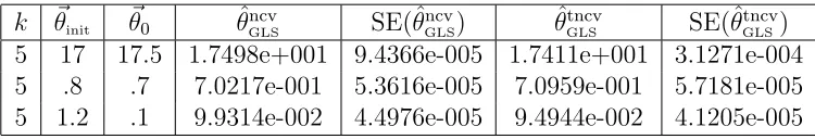
for each method and error structure are given in Tables 1-4 (the superscript tcv and tncv denote the estimate obtained using the truncated data set). As expected, both methods do

a good job of estimating ~θ0, however the error structure was not always correctly specified

since incorrect asymptotic formulas were used in some cases.

Table 1: Estimation using the OLS procedure with constant variance data for k = 5.

k ~θinit ~θ0 θˆcvOLS SE(ˆθ

cv

OLS) θˆ

tcv

OLS SE(ˆθ

tcv

OLS)

5 17 17.5 1.7500e+001 1.5800e-003 1.7494e+001 6.4215e-003

5 .8 .7 7.0018e-001 4.2841e-004 7.0062e-001 6.5796e-004

5 1.2 .1 9.9958e-002 3.1483e-004 9.9702e-002 4.3898e-004

Table 2: Estimation using the GLS procedure with constant variance data for k = 5.

k ~θinit ~θ0 θˆcvGLS SE(ˆθ

cv

GLS) θˆ

tcv

GLS SE(ˆθ

tcv

GLS)

5 17 17.5 1.7500e+001 1.3824e-004 1.7494e+001 9.1213e-005

5 .8 .7 7.0021e-001 7.8139e-005 7.0060e-001 1.6009e-005

(20)

Table 3: Estimation using the OLS procedure with nonconstant variance data fork = 5.

k ~θinit ~θ0 θˆncvOLS SE(ˆθ

ncv

OLS) θˆ

tncv

OLS SE(ˆθ

tncv

OLS)

5 17 17.5 1.7499e+001 2.2678e-002 1.7411e+001 7.1584e-002

5 .8 .7 7.0192e-001 6.1770e-003 7.0955e-001 7.6039e-003

5 1.2 .1 9.9496e-002 4.5115e-003 9.4967e-002 4.8295e-003

Table 4: Estimation using the GLS procedure with nonconstant variance data fork = 5.

k ~θinit ~θ0 θˆncvGLS SE(ˆθ

ncv

GLS) θˆ

tncv

GLS SE(ˆθ

tncv

GLS)

5 17 17.5 1.7498e+001 9.4366e-005 1.7411e+001 3.1271e-004

5 .8 .7 7.0217e-001 5.3616e-005 7.0959e-001 5.7181e-005

5 1.2 .1 9.9314e-002 4.4976e-005 9.4944e-002 4.1205e-005

When the OLS method was applied to nonconstant variance data and the GLS method was applied to constant variance data, the residual plots given below do reveal that the error

structure was misspecified. For instance, the plot of the residuals for ˆθncv

OLS given in Figures

4 and 5 reveal a fan shaped pattern, which indicates the constant variance assumption is

suspect. In addition, the plot of the residuals for ˆθcv

GLS given in Figures 6 and 7 reveal

an inverted fan shaped pattern, which indicates the nonconstant variance assumption is

suspect. As expected, when the correct error structure is specified, the i.i.d. test and the

model dependence test each display a random pattern (Figures 2, 3 and Figures 8, 9). Also, included in the right panel of Figures 2 - 9 are the residual plots with the truncated data sets. In those plots only model values between one and seventeen were considered (i.e.

1_≤yj ≤ 17). Doing so removed the dense vertical lines in the plots with f(tj,θˆ) along the

(21)

Figure 2: Residual plots: Original and truncated logistic curve for ˆθcv

OLS with k = 5.

0 5 10 15 20 25

−0.2 −0.15 −0.1 −0.05 0 0.05 0.1 0.15 0.2

Time

Residual

Residual vs. Time with OLS & CV Data

3 4 5 6 7 8 9 10 11 12 13

−0.2 −0.15 −0.1 −0.05 0 0.05 0.1 0.15 0.2

Time

Truncated Residual

Residual vs. Time with OLS & Truncated CV Data

Figure 3: Original and truncated logistic curve for ˆθcv

OLS with k = 5.

0 2 4 6 8 10 12 14 16 18

−0.2 −0.15 −0.1 −0.05 0 0.05 0.1 0.15 0.2

Model

Residual

Residual vs. Model with OLS & CV Data

0 2 4 6 8 10 12 14 16 18

−0.2 −0.15 −0.1 −0.05 0 0.05 0.1 0.15 0.2

Truncated Model

Truncated Residual

(22)

Figure 4: Original and truncated logistic curve for ˆθncv

OLS with k = 5.

0 5 10 15 20 25

−3 −2 −1 0 1 2 3

Time

Residual

Residual vs. Time with OLS & NCV Data

3 4 5 6 7 8 9 10 11 12 13

−3 −2 −1 0 1 2 3

Time

Truncated Residual

Residual vs. Time with OLS & Truncated NCV Data

OLS with k = 5.

0 2 4 6 8 10 12 14 16 18

−3 −2 −1 0 1 2 3

Model

Residual

Residual vs. Model with OLS & NCV Data

0 2 4 6 8 10 12 14 16 18

−3 −2 −1 0 1 2 3

Truncated Model

Truncated Residual

(23)

GLS with k = 5.

0 5 10 15 20 25

−1 −0.8 −0.6 −0.4 −0.2 0 0.2 0.4 0.6 0.8 1

Time

Residual/Model

Residual/Model vs. Time with GLS & CV Data

3 4 5 6 7 8 9 10 11 12 13

−0.15 −0.1 −0.05 0 0.05 0.1

Time

Truncated Residual/Model

Residual/Model vs. Time with GLS & Truncated CV Data

GLS with k = 5.

0 2 4 6 8 10 12 14 16 18

−1 −0.8 −0.6 −0.4 −0.2 0 0.2 0.4 0.6 0.8 1

Model

Residual/Model

Residual/Model vs. Model with GLS & CV Data

0 2 4 6 8 10 12 14 16 18

−0.15 −0.1 −0.05 0 0.05 0.1

Truncated Model

(24)

GLS with k = 5.

0 5 10 15 20 25

−0.2 −0.15 −0.1 −0.05 0 0.05 0.1 0.15 0.2

Time

Residual/Model

Residual/Model vs. Time with GLS & NCV Data

3 4 5 6 7 8 9 10 11 12 13

−0.2 −0.15 −0.1 −0.05 0 0.05 0.1 0.15 0.2

Time

Residual/Model vs. Time with GLS & Truncated NCV Data

GLS with k = 5.

0 2 4 6 8 10 12 14 16 18

−0.2 −0.15 −0.1 −0.05 0 0.05 0.1 0.15 0.2

Model

Residual/Model

Residual/Model vs. Model with GLS & NCV Data

0 2 4 6 8 10 12 14 16 18

−0.2 −0.15 −0.1 −0.05 0 0.05 0.1 0.15 0.2

Truncated Model

(25)

In addition to the residual plots, we can also compare the standard errors obtained for

each simulation. At a quick glance of Tables 1 - 4, the standard error of the parameter K in

the truncated data set is larger than the standard error of K in the original data set. This

behavior is expected. If we remove the “flat” region in the logistic curve, we actually discard

measurements with high information content about the carrying capacity K [4]. Doing so

reduces the quality of the estimatorK. Another interesting observation is that the standard

(26)

5

Pneumococcal Disease Dynamics Model

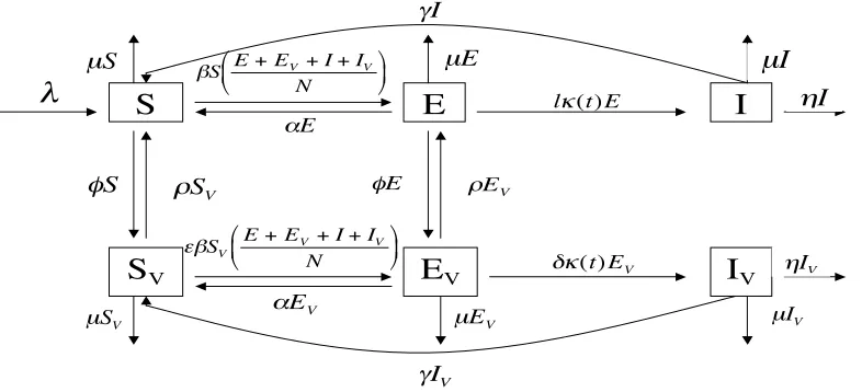
To explore these ideas in the context of epidemiology, we discuss a population level model of pneumococcal disease dynamics as an example. This model has previously been applied to surveillance data available via the Australian National Notifiable Diseases Surveillance System in [32]. Monthly case notifications of invasive pneumococcal disease (IPD) and annual vaccination information were used to estimate unknown model parameters and to assess the impact of a newly implemented vaccination policy. Here we illustrate, with this example, the effects of incorrect versus correct statistical models assumed to represent observed data in reporting parameter values and their corresponding standard errors. Most importantly, we discuss relevant residual plots and how to use these to determine if reasonable assumptions on observed error have been made.

Figure 10: Pneumococcal infection dynamics with vaccination.

"

S E+EV+I+IV

N

# $

% &

' (

"E

"#S_V E+EV+I+IV

N $

%

& '

( )

"E

V

S

_V

E

_V

I

"S "E

"#(t)E_V

l_"₍t₎E

"I

"S

V "EV

I

_V "I_V

"I_V

µ_I

µS µ_E

µS

V µEV µ

I V

In this model, shown in Figure 10, individuals are classified according to their epidemi-ological status with respect to invasive pneumococcal diseases, which include pneumonia,

bacteremia, meningitis and are defined as the presence of Streptococcus pneumoniae in any

normal sterile fluid in the body. Individuals are considered susceptible, or in the S class,

in the absence of this bacteria. The E class represents individuals whose nasopharyngeal

regions are asymptomatically colonized byS. pneumoniae, a stage that is typically transient,

but always precedes infection. Should a colony ofS. pneumoniaebe successful in establishing

an infection, the individual then exhibits a clinical condition described above, and is then

considered infected or in the I class. We consider vaccines which prevent progression to

infection, or possibly, asymptomatic colonization. This protection is not complete, and the

efficacy with which this is accomplished is 1−δ and 1−ǫ, respectively. Once vaccinated,

individuals may enter any of the epidemiological states, SV, EV, and IV, although they do

(27)

dS

dt =λ−βS

E+EV +I+IV

N +αE+γI−φS+ρSV −µS (56) dE

dt =βS

E+EV +I+IV

N −αE−lκ(t)E−φE+ρEV −µE (57) dSV

dt =φS−ǫβSV

E+EV +I+IV

N +αEV +γIV −ρSV −µSV (58) dEV

dt =ǫβSV

E+EV +I+IV

N −αEV +φE−ρEV −δκ(t)EV −µEV (59) dI

dt =lκ(t)E−(γ+η+µ)I (60) dIV

dt =δκ(t)EV −(γ+η+µ)IV. (61)

Seasonality of invasive pneumococcal diseases has been observed and studies support a

seasonal infection rate,κ, rather than a seasonal effective contact rate,β. Thus, we assume

the form

κ(t) =κ0(1 +κ1cos[ω(t−τ)]),

forκ(t) to reflect seasonal changes in host susceptibility to pneumococcal infection.

5.1

Statistical Models of Case Notification Data

Monthly case notificationsf(tj, ~θ) are best represented as integrals of the new infection rates,

f(tj, ~θ) =

Z tj+1

tj

[lκ(s)E(s) +δκ(s)EV(s)]ds,

(including those in the vaccinated class) over each month, since they represent the number of cases reported during the month and do not provide any information on how long individuals

remain in an infected state. We use these data to estimate~θ= (β, κ0, κ1)T. Before using the

model with surveillance data, we test the model and methodology capabilities with simulated “data”. Following the procedures in the logistic example discussions in Section 4, we generate data according to two statistical models:

Yj =f(tj, θ0) +ǫj, (62)

Yj =f(tj, θ0)(1 +ǫj), (63)

for j = 1, ..., n, where ~θ0 are the ‘true’ values of the parameters used to generate the data.

In both (62) and (63), the ǫj are independent and identically distributed (i.i.d.) random

variables with E[ǫj] = 0 and var(ǫj) = σ02. In model (62), however, the residual is then

(28)

will refer to this error with constant variance, or CV. The second case, (63), has residuals

of the form Rj =Yj−f(tj, ~θ0) = ǫjf(tj, ~θ0), so the residual is actually proportional to the

model, f(tj, ~θ0), at each time pointtj, and thus this is an example of error withnonconstant

variance, or NCV. We note that in this case E[Rj] = 0 and var(Rj) =σ02f2(tj, ~θ0) or _f₍_tRj

j,~θ0)

has mean zero and variance σ2

0.

For illustration, we consider the same four cases as with the logistic example in Section 4:

1. OLS estimation of ˆθ using data generated by model (62) with constant variance

obser-vational error: θOLS(YCV),

2. OLS estimation of ˆθ using data generated by model (63) with nonconstant variance

observational error: θOLS(YN CV),

3. GLS estimation of ˆθ using data generated by model (62) with constant variance

obser-vational error: θGLS(YCV),

4. GLS estimation of ˆθ using data generated by model (63) with nonconstant variance

observational error: θGLS(YN CV).

We compare the parameter estimates ˆθ and standard errors SE(ˆθ) obtained in each case.

Further we discuss how to interpret plots of rj =yj−f(tj,θˆ) versus tj and f(tj,θˆ) to assess

whether reasonable assumptions have been made in assuming the statistical model for the data.

5.2

Inverse Problem Results: Simulated Data

Data were generated with n = 60 time points (equivalent to five years of data), with the set

of parameters

~θ0 =

 

β κ0

κ1

 =

 

1.5 1.4e−3

0.55

 .

Error was added to the forward solution according to two statistical models, as described in Section 5.1. In the case of constant variance observational error, the error is scaled to the magnitude of the model but not in a time-dependent manner. In this case we generated noisy

data by sampling from a N(0,1) distribution (we could of course have sampled from any

other random variable). Therefore, for constant variance error of about k% of the average

magnitude of the f(tj, ~θ0),

ǫj ∼

k

100avgjf(tj, ~θ0)N(0,1).

So in this caseǫj ∼ N(0,[₁₀₀k avgjf(tj, ~θ0)]2) withǫj (and also Rj)i.i.d.In the second

statis-tical model, the error depends on time and is scaled by the model at each time point, i.e.,

(29)

Table 5: Parameter estimates from data with constant variance CV error.

~θ ~θ0 ~θ_init θˆOLS SE(ˆθOLS) θˆGLS SE(ˆθGLS)

β 1.5 1.55 1.4845 0.038 1.51186 0.017

κ0 1.4e−3 1.3e−3 1.4188e−3 2.1e−4 1.3203e−3 1.2e−4

κ1 0.55 0.65 0.56203 0.050 0.56047 0.019

RSS 1.6831e4 ₁_.₇₂₂_e4

Rj =f(tj, ~θ0)ǫj ∼f(tj, ~θ0)

k

100N(0,1),

with ǫj ∼ N(0,[₁₀₀k f(tj, ~θ0)]2), and again the ǫj are i.i.d.,but now the Rj are not i.i.d.This

enables us to compare different types of error on the same scale: one independent of time and observation magnitude, and one dependent on observation magnitude, and thus time.

With the present examples, we have taken k = 10.

The results from using an OLS and GLS estimator with data generated with constant variance error are displayed in Table 5, and the fitted model solutions displayed in Figure

11. Both estimators do an arguably similar job at producing the true values, that is ˆθOLS

and ˆθGLS are comparably close to θ0. The standard errorsSE(ˆθGLS) for the GLS estimator

however, are all smaller, and seem to indicate that the corresponding estimates are more “reliable”. This, however, is not true because they are based on incorrect formulae, as we shall see in our examination of the error plots for both of these cases. Note that from Figure

11 and the residual sum of squares, RSS, in both cases, there is no clear argument from

these results as to which estimator is better suited for use with the data.

Figure 11: Best fit model solutions to monthly case notifications with constant variance CV error.

0 10 20 30 40 50 60

0 50 100 150 200 250 300 350

Best fit model solution using OLS estimation

Time t

j (months)

Cases

0 10 20 30 40 50 60

0 50 100 150 200 250 300 350

Best fit model solution using GLS estimation

Time t

j (months)

(30)

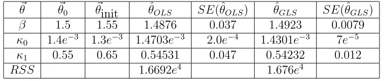
Table 6: Parameter estimates from data with nonconstant variance NCV error.

~θ ~θ0 ~θ_init θˆOLS SE(ˆθOLS) θˆGLS SE(ˆθGLS)

β 1.5 1.55 1.4876 0.037 1.4923 0.0079

κ0 1.4e−3 1.3e−3 1.4703e−3 2.0e−4 1.4301e−3 7e−5

κ1 0.55 0.65 0.54531 0.047 0.54232 0.012

RSS 1.6692e4 ₁_.₆₇₆_e4

Figure 12: Best fit model solutions to monthly case notifications with nonconstant variance NCV error.

0 10 20 30 40 50 60

50 100 150 200 250 300 350

Best fit model solution using OLS estimation

Time t_j (months)

Cases

0 10 20 30 40 50 60

50 100 150 200 250 300 350

Best fit model solution using GLS estimation

Time t_j (months)

Cases

When OLS and GLS estimation are each used with data with nonconstant variance error, the parameters and standard errors in Table 6 are obtained, and the plot of these model solutions over the generated data is given in Figure 12. Again, one estimator does not do a clearly better job over the other in terms of predicting parameter values closer to those used to generate the data. However, again, the standard errors from the GLS estimation are smaller as compared to those of the OLS estimation. From this, it would seem that the GLS estimation would always give ‘better’ parameter values, or do a better job at producing reliable results. However, we know that in the case of constant variance error, the GLS estimation makes some incorrect assumptions on the data generation and therefore, the standard errors reported there would give a false sense of confidence in the values (indeed they are based on incorrect asymptotic formulae).

5.2.1 Residual Plots

Here we illustrate use of residual plots to investigate whether our assumptions on the errors

incurred in observation of data are correct - that is, whether theǫjarei.i.d.for allj = 1, ..., n,

(31)

Section 4, if the errors are i.i.d. then a plot of the residuals rj = yj −f(tj,θˆ) versus time

tj should show no discernible pattern. Similarly, a plot of the residual rj as a function of

the model values f(tj,θˆ) should be random if there is no relationship between these two

quantities. While use of the OLS estimation tacitly assumes the statistical model (62), and therefore the residual is a realization of the error random variable, this is not true of the

GLS estimation. In that case, the assumed statistical model is shown in (62) with ǫj i.i.d.

but the residualrj are not i.i.d.for all j = 1, ..., n. Therefore, in the case of GLS we should

investigate plots of the the residual/model values,Rj = Yj

−f(tj,θ0)

f(tj,θ0) instead of the residuals.

Figure 13: Residual (rj = yj −f(tj,θˆ)) plots of the OLS estimation with CV data (ǫj =

Yj−f(tj, ~θ0)); Left: nontruncated, Right: truncated.

0 10 20 30 40 50 60

−50 −40 −30 −20 −10 0 10 20 30 40

OLS estimation with CV Data

Time t

j (months)

Residual

0 2 4 6 8 10 12

−20 −15 −10 −5 0 5 10 15 20 25

Time t

j (months)

Residual

50 100 150 200 250 300

−50 −40 −30 −20 −10 0 10 20 30 40

Model f(t

j, θ)

Residual

50 100 150 200 250 300

−20 −15 −10 −5 0 5 10 15 20 25

Model f(t

j, θ)

Residual

In Figure 13, we see the relationship between the residuals and time, and that between residuals and the model values when the OLS estimation procedure is applied to data which has been generated with constant variance error. In both the top and bottom panels on

the left, the full set of n = 60 points are used, while on the right hand side, only one

(32)

pattern, so the errors are clearly i.i.d. But in the bottom left plot, we observe clustering of residuals around certain model values, although there is no clear pattern in the dependent

variable, just in the independent variable, f(tj,θˆ). However, we recognize that this is due

to the seasonality of the data and model, so that at regular repeated time points over many periods, there are going to be repeated values of the model. As evidence of this, we see that when only one period is plotted (the bottom right panel), a random pattern is seen, and we confirm that the errors are not dependent on the model values. Thus, if there are vertical bands on a plot such as this, it can be attributed to certain model values repeating and does not indicate any dependence of the error on the model value. To check, one can simply reduce the number of data points used in the estimation so that there are few or no repeated values.

Figure 14: Residual (rj = yj −f(tj,θˆ)) plots of the OLS estimation to NCV data (ǫj =

Yj−f(tj,~θ0)

f(tj,~θ0) ); Left: nontruncated, Right: truncated.

0 10 20 30 40 50 60

−60 −40 −20 0 20 40 60

OLS estimation with NCV Data

Time t

j (months)

Residual

0 2 4 6 8 10 12

−30 −20 −10 0 10 20 30

Time t

j (months)

Residual

80 100 120 140 160 180 200 220 240 260 280

−60 −40 −20 0 20 40 60

Model f(t

j, θ)

Residual

80 100 120 140 160 180 200 220 240 260 280

−30 −20 −10 0 10 20 30

Model f(t

j, θ)

Residual

(33)

these graphs (Figure 14) do not show a random pattern. While there is no clear relation-ship, there is some randomness in the residuals, and the band of residuals are tighter, not homogeneously distributed across the plot as in Figure 13. The dependence of the residuals

on model value magnitude (seen in the bottom panels) is apparent as the rj clearly increase

with increasing model values, producing a fan shape. In this case the OLS estimation is used incorrectly, and the residual plots exhibit a clear dependence on model values and do not confirm independence from time.

Figure 15: Residual/Model ( rj

f(tj,θˆ)) plots of the GLS estimation to CV data (ǫj = Yj −

f(tj, ~θ0)); Left: nontruncated, Right: truncated.

0 10 20 30 40 50 60

−8 −6 −4 −2 0 2 4

6x 10

−3 GLS estimation with CV Data

Time t

j (months)

Residual/Model

0 2 4 6 8 10 12

−1.5 −1 −0.5 0 0.5 1 1.5 2 2.5

3x 10

Time t

j (months)

Residual/Model

50 100 150 200 250 300

−8 −6 −4 −2 0 2 4

6x 10

Model f(t

j, θ)

Residual/Model

50 100 150 200 250 300

−1.5 −1 −0.5 0 0.5 1 1.5 2 2.5

3x 10

Model f(t

j, θ)

Residual/Model

(34)

plots in Figure 15 reveal a tight band of points in the rj

f(tj,θˆ) versus tj plots and the reverse

fan shape of the plot of the residual/model rj

f(tj,θˆ) versus the model values f(tj,

ˆ

θ). This

indicates that the relations which give us the parameter estimates and their standard errors no longer hold and we are essentially reporting incorrect values. As we saw in Section 5.2, while the parameter estimates may not necessarily be poor, the reliability provided by the standard errors is incorrect.

Figure 16: Residual/Model ( rj

f(tj,θˆ)) plots of the GLS estimation to NCV data (ǫj =

Yj−f(tj,~θ0)

f(tj,~θ0) ); Left: nontruncated, Right: truncated.

0 10 20 30 40 50 60

−0.2 −0.15 −0.1 −0.05 0 0.05 0.1 0.15 0.2

GLS estimation with NCV Data

Time t

j (months)

Residual/Model

0 2 4 6 8 10 12

−0.2 −0.15 −0.1 −0.05 0 0.05 0.1 0.15

Time t

j (months)

Residual/Model

80 100 120 140 160 180 200 220 240 260 280

−0.2 −0.15 −0.1 −0.05 0 0.05 0.1 0.15 0.2

Model f(t

j, θ)

Residual/Model

80 100 120 140 160 180 200 220 240 260 280

−0.2 −0.15 −0.1 −0.05 0 0.05 0.1 0.15

Model f(t

j, θ)

Residual/Model

When the GLS estimator is used appropriately, however, the randomness of the error plots suggest reasonability of assumptions, as seen in Figure 16. Here, the error in the data has been generated proportional to the model values, and therefore, not longitudinally

constant. So when we plot the ratios yj−f(tj,θˆ)

f(tj,θˆ) , we allow for this dependence and see the

(35)

seen by the bottom right panel, where the repetitions have been excluded from the data set.

5.3

Inverse Problem Results: Australian Surveillance Data

Using the iterative weighted least squares procedure described in Section 2.4.2, we carried out inverse problem calculations with the model and observations as outlined in the previous section using Australian IPD data in place of the simulated data. In this case we assumed constant variance noise in the data and hence used WLS , e.g., see (27), for our estimation procedure. Details are given in [32]. We discuss here the case where we used data for the

period 2002-2004 (36 months of monthly data n1 = 36, and n2 = 6 of annual vaccinated or

unvaccinated cases) and e