Report No. 450
AN INTEGRATED FRAMEWORK FOR ASSESSING THE DYNAMICS OF POPULATION GROWTH, LAND USE AND CLIMATE CHANGE FOR URBAN WATER RESOURCES MANAGEMENT
By
Emily Zechman Berglund and Sankar Arumugam
Department of Civil, Construction and Environmental Engineering North Carolina State University
Raleigh, NC
UNC-WRRI-450
The research on which this report is based was supported by funds provided by the North Carolina General Assembly and/or the US Geological Survey through the NC Water Resources Research Institute.
Contents of this publication do not necessarily reflect the views and policies of WRRI, nor does mention of trade names or commercial products constitute their endorsement by the WRRI, the State of North Carolina, or the US Geological Survey.
This report fulfills the requirements for a project completion report of the Water Resources Research Institute of The University of North Carolina. The authors are solely responsible for the content and completeness of the report.
1 ABSTRACT
The management of water resources requires careful planning to balance water supply and demand. Under increasing population growth and land use change through urbanization, water shortages may become increasingly frequent, and climate change will alter the availability and timing of water from expected levels. While long-term water supply planning is conventionally based on projections of population growth, demands, and system capacity under a stationary climate, the sustainability of water resources depends on the dynamic interactions among the environmental, technological, and social characteristics of the water system and local population. These interactions can cause supply-demand imbalances at various temporal scales, and the response of consumers to water use regulations will impact future water availability. To address the challenges of water resources management and provide insight to system dynamics, new modeling is needed that goes beyond simple assumptions on water availability, population growth and demand increases, to explicitly incorporate the feedbacks among these systems and their impacts on water availability. The research described here develops an integrated urban water management framework with capabilities to evaluate demand-side and supply-side management strategies. This research establishes a dynamic modeling approach to understand the supply-demand dynamics and feedbacks arising from urban growth dynamics, consumer behaviors, and potential changes in climate and land use. An agent-based modeling approach is developed to couple models of consumers and utility managers with watershed and reservoir models. Households are represented as agents, and their water use behaviors are represented as rules. A deterministic end use model is used to simulate indoor demands, and landscaping demands are calculated based on irrigation requirements of crops and behaviors of end users. A population growth model is used to simulate an increasing number of household agents. A water utility manager agent enacts water use restrictions, based on fluctuations in the reservoir water storage. Water balance in a reservoir is simulated, and climate scenarios are used to test the sensitivity of water availability to changes in precipitation and temperature. The integrated framework provides insight for water utility operators and stakeholders about the interactions of management strategies, climate change, population growth, and consumer behaviors, and the impact that these behaviors have on long-term water supply sustainability. The framework is applied to the Falls Lake water supply system to analyze the accuracy of the modeling
2 ACKNOWLEDGEMENTS
3 1 INTRODUCTION
Urban water resources should be managed sustainably to achieve an appropriate balance between water demand and supply. This balance is increasingly difficult to sustain as urban areas increase in size, and precipitation decreases due to climate change. Traditionally, water shortages are managed by supply management, which is based on the assumption that economic growth generates new demands. Supply management does not control demand, but increases the supply to meet demands. This approach leads to the depletion of freshwater reserves and the
construction of large infrastructure systems comprised of pipe networks and pumping stations. Continuing to use a supply management approach is not feasible for many utilities due to additional objectives and goals that should be considered in planning, such as greenhouse gas emissions, energy requirements, decaying infrastructure, and water shortages. Subsequently, demand management has emerged as a promising paradigm for sustainable management of water resources. Demand management focuses on reducing demands through water pricing,
educational campaigns, incentives and rebates for water-saving technologies, regulations, and metering. Demand-side strategies have the potential to significantly reduce demands, but they rely on changes in human behavior, and the performance is impacted by social factors.
Management strategies are typically developed using linear projections of population growth, demands, and system capacity under a stationary climate and a homogeneous population of consumers. The sustainability of water resources, however, may be affected by the dynamic interactions among the environmental, technological, and social characteristics of the water system and local population. The response of water consumers to demand management strategies can affect the performance of management, and the dynamic adoption of water-efficient
appliances can impact the evolution of water availability. These interactions can cause supply-demand imbalances that may not be predictable using traditional engineering models and assumptions of a stationary climate. Single-family residential customers typically comprise the largest water demand sector in utilities across the United States. Regional variations in climate across the country impact the relative consumption of the single-family residential customer class as well as its end use demand patterns.
4
management strategies, climate change, population growth, and consumer behaviors, and the impact that these behaviors have on long-term water supply sustainability.
5
2 CHANGES TO THE PROPOSED PLAN OF WORK
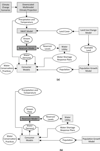
Preliminary research was conducted that led to changes in the plan of work, as described in the proposal. A pictorial depiction of the changes between the framework that was originally proposed and the work that was completed are given in Fig. 1. Namely, the completed
framework does not include land use change modeling, hydrologic modeling, and downscaled climate data. Reasons for these changes are described in Sections 2.1 and 2.2. The omission of these tasks provided the resources to improve the modeling approach, validate the approach for existing data sets, and calculate sustainability of alternative drought management strategies (summarized in Section 2.3).
The framework that was completed is described in explicit detail in Section 3. The goal of this section is to describe changes in the proposed framework.
2.1 OMIT LAND USE CHANGE MODELING
The framework, as it was originally proposed, would simulate land use change due to urbanization and its effects on the flows into the Falls Lake Reservoir. Preliminary
investigations explored the forecasted land use changes, through the year 2030, as described by the City of Raleigh (2009). This report demonstrated that the land use changes that are expected in the City of Raleigh would result primarily in densification of land use, or infill, and new development in the east and southeast. Because the land use change that is expected would not impact the watershed that contributes to Falls Lake, it was not included in the modeling
framework.
2.2 OMIT FALLS LAKE WATERSHED MODELING AND CLIMATE DOWN-SCALING
6
2.3 INCLUDE METHODS FOR EVALUATING MODEL PERFORMANCE AND SUSTAINABILITY OF DROUGHT RESPONSE PLANS
The completed modeling framework coupled agent-based models with models of the reservoir release and storage. The revised research plan provided the flexibility and research effort to explore the accuracy of the modeling approach. The studies that apply ABM for urban water supply simulation (Rixon et al. 2007; Klotz and Hiessl 2005; Schwarz and Ernst 2009; Athanasiadis et al. 2005; Galan et al. 2009; Galan et al. 2008) explore what-if scenarios and generate insight about the effects of water conservation, but they have not validated ABM approaches as accurate, beyond testing varying degrees of social influence in a population (Moss and Edmonds 2005). In general, ABM and system dynamic models are often criticized for relying on informal and subjective validation or no validation at all (Edmonds and Chattoe 2005). Validating ABM approaches for simulating social is challenged by several difficulties: (1) path dependencies and the stochastic nature of human behavior models make point predictions impossible; (2) the domains in which these models are applied lack consolidated data sources; and (3) social system models are complex with huge feature spaces (Pahl-Wostl 1995; Bharathy and Silverman 2012). ABM is typically validated using internal consistency checks, which ensure that the microspecifications of behaviors are adequate representations of actors’ activities (Gilbert 2007; Gratch and Marsella, 2004). External evaluation has been used in a limited set of studies to quantitatively assess observed features of aggregate time series of output (Moss and Edmonds 2005) and the occurrence of false/true positives in predicting discrete events that emerge at the macroscopic level (Bharathy and Silverman 2012). The research that was conducted evaluated the time series of modeled output to validate the ABM approach beyond water systems studies in the existing literature.
The second research effort that was conducted beyond what was originally proposed was the evaluation of drought management strategies using specified sustainability metrics. Drought management strategies can be evaluated simply by calculating the storage of water in the
7
Figure 1. (a) Originally proposed modeling framework, including hydroclimatic models, reservoir system model, and models of social behaviors and processes. Information is passed among models. (b) The modeling framework as implemented in the completed research plan. !"#$%&'()*% +,*)"-% ./'0% 1'23/"4'#% 5",)*% 6)-"#$% !"#$%78)%&9"#:)% ;'$)/% &'#83-)*%
;'$)/8% 1'23/"4'#%<*'0,9%;'$)/%
=(">/"?/)% !"#$% 5",)*%+9'*,":)% @)82'#8)%1/"#8% 5",)*% 74/>,A% @)8)*('>*% !)()/8% &/>-",)% &9"#:)% +B)#"*>'8% 6'0#8B"/)$% ;3/4-'$)/% &/>-",)%1*'C)B4'#% 1*)B>2>,"4'#%"#$% D)-2)*",3*)% +5=D%;'$)/%% @)8)*('>*%;'$)/% 5",)*% &'#8)*("4'#% 1*"B4B)8% !"#$ +,*)"-% ./'0% 1'23/"4'#% 5",)*% 6)-"#$% &'#83-)*%
;'$)/8% 1'23/"4'#%<*'0,9%;'$)/%
8 3 METHODS
An agent-based modeling framework is developed to simulate urban water resources as a complex adaptive system (Holland 1995). Agent-based modeling is an approach for simulating networks comprised of autonomous, interacting agents (Miller and Page 2007). The dynamic interactions among agents and a shared environment are modeled to simulate the emergence of system-level properties. Agent-based modeling has been developed for exploring the influence of human behaviors and decision-making on water resources systems. For example, agent-based modeling frameworks were applied to study rules for the expansion of water infrastructure (Tillman et al. 2005) and to model a population of customers with changing water demands (Athanasiadis et al. 2005; Rixon and Burns 2007; Galan et al. 2009).
The agent-based modeling framework is described in Section 2.1. The agent-based modeling framework is used to simulate historic data and projections of water supply for management and climate scenarios for Raleigh, NC. Application and results are described in Section 3, and the modeling framework is described generically in Section 2.1, as it could be applied for any municipality. The metrics that are used to evaluate the accuracy of the model for simulated historic data are described in Section 2.2. Metrics that are used to evaluate the sustainability of management scenarios are described in Section 2.3.
3.1 AGENT-BASED MODELING FRAMEWORK
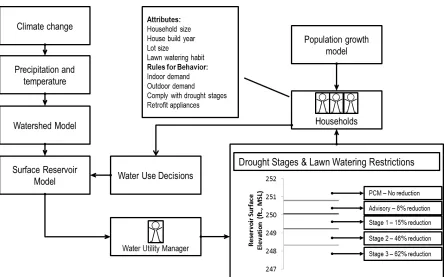
The framework is composed of subcomponents that capture various influential socio-technical aspects of the water resources in a metropolitan area. Before describing the details of each of the sub-models, it is important to explain the general structure of the overall model: the agents and the technical models as the shared environment. The model includes household agents and a water utility manager agent (Fig. 2). Household agents withdraw water from the reservoir, and a hydrologic model is used to simulate runoff from the contributing watershed based on
climatological data. Household agents receive alerts from the water utility manger agent about the level of water use restrictions, which are enacted when storage in the reservoir drops below pre-defined stages. This model extends a framework that was developed to simulate population growth, land use change, and water conservation for the City of Arlington, Texas (Giacomoni et al. 2013; Kanta and Zechman 2014). The model is implemented in Java using MASON agent-based simulation libraries (Luke et al. 2005).
9
Figure 2. ABM framework. PCM is Permanent Conservation Measures.
3.1.1 Household agents
Households are simulated as agents, with properties and behavioral rules to simulate household-level demands. Household size, house built year, and lot size are considered as properties, and rules are encoded to calculate indoor water use, adaptive outdoor water use, retrofitting water appliances, and lawn watering habits. The total demand for a household agent is the sum of indoor end uses and the outdoor end use, described below.
Attributes can be initialized using historic information and projections. Household agents are assigned the number of residents using demographic information and distribution of household size based on U.S. Census Bureau.
Indoor end use demand model
10
The end use model estimates the water use of each end-use per day per household as the product of the water use rate of the end-use and the frequency of use (number of uses per person per day), using volumes as shown in Table 1, as reported by Vickers (2001). Daily water demands are multiplied by the number of days per month to obtain monthly demands. Daily demands are calculated per person (Fig. 3) to explore the change in demands from pre-1950 to the present, due to the penetration of more water-efficient appliances. Water Sense appliances provide the most water-efficient appliances, and they are adopted by agents after 2001 (the time of
publication of the report). Household agents replace toilets, showerheads, faucets, clothes washer, and washing machines with more efficient appliances after the appliance life span has expired, and this changes the indoor water demand volume. The life span of each appliance is simulated as 30 years. Each agent is assigned a set of appliances based on the build year of its house. Each agent replaces appliances with more efficient appliances every 30 years.
Table 1. Water demand volume for household indoor end uses (Vickers 2001) Water Appliance/fixtures
Showerhead (gpm)
Toilet (gpf)
Faucet (gpm)
Dishwasher (gpl)
Clothes Washer (gpl)
Pre-1950 4.3 7 3.3 14 56
1950s-1980 4.3 5.5 3.3 14 56
1980-1994 1.8-2.7 3.5-4.5 1.8-2 9.5-14 43-51
1994-present 1.7 1.6 1-1.7 7-10.5 27-39
Water Sense 1.4 1 1 4.5 27
Frequency of Use (per capita)
5.3 (min/day)
5.1 (flush/day)
8.1 (min/day)
0.1 (load/day)
11
Figure 3. Daily water demand for indoor end use appliances per person
Leakage is also calculated as an end-use to represent water that is lost due to cracks in pipes and leaky appliances. Instead of a deterministic end use calculation, as shown above, leakage is estimated using a probabilistic distribution based on a study conducted in California in 2011 (DeOreo et al. 2011) (Fig. 4). Leakage is not updated as homes are retrofitted, due to a lack of data to describe changes in leakage rates with retrofits. The distribution of indoor water volume across all end uses, as reported by DeOreo et al. (2011), is shown in Fig. 5. Leakage represents approximately 18% of indoor water consumption.
Figure 4. Distribution of leakage rates across households (DeOreo et al. 2011). 0
5 10 15 20 25 30 35 40
Pre-‐1950 1950s-‐1980 1980-‐1994 1994-‐present WaterSense
Wa
ter U
se
(gal
lo
n p
er d
ay
p
er p
erso
n)
Showerhead Toilet Faucets Dishwashers Cloth Washers Clothes Washers
0% 10% 20% 30% 40% 50% 60% 70% 80% 90% 100%
0% 5% 10% 15% 20% 25% 30% 35% 40% 45% 50%
10 20 30 40 50 60 70 80 90 100 110 120 130 140 150 160 170 180 190 200
Mo re Cu m ul a5 ve Fr eq ue nc
y
%
of
H
ou
se
s
Leakage Rate (gphd)
12
Figure 5. Distribution of indoor water volume that is consumed by indoor end use appliances (DeOreo et al. 2011).
End use volumes for baths and other end uses are calculated based on the mean and standard deviation (DeOreo et al. 2011). Other end uses are those that simply do not fit neatly into any other category. Like leakage end-use, the volume for other and bathing end uses are not updated through retrofitting, due to a lack of data to describe changes in volume. End uses for bath and other are calculated as follows.
3.2 1 gphd
Bath= ± (1)
7.8 2 gphd
Other = ± (2)
where gphd stands for gallons per household per day, Bath is the volume of water used for baths,
and Other is the volume of water used for other end uses. Volumes are reported as the average + the standard deviation. Bath represents approximately 2% of indoor water demands, and other uses represent approximately 2% of indoor water demands (Fig. 5).
Outdoor demand model
A significant portion of residential outdoor demand is used for garden watering. The following approach calculates outdoor demand as a function of climatic data and water demands for landscaping. Other outdoor demands, such as swimming pools and washing vehicles and driveways, are neglected.
20%
20%
19% 18%
18%
2% 2% 1%
Toilet
Shower
Faucet
Clothes Washer
Leaks
Other
Bath
13
The water demands for landscape irrigation are calculated using a theoretical irrigation model,
which is based on a soil-water budget model. The theoretical irrigation requirement (TIR) is
calculated for each agent, or household, based on the area of land dedicated to each plant type, evapotranspiration and precipitation data, efficiency of irrigation technologies, and crop coefficient for each plant type.
net
0.624 o A crop
TIR ET K
Eff
⎛ ⎞
= × ×⎜ ⎟×
⎝ ⎠ (3)
where
TIR = theoretical irrigation requirement (gal)
ETo net = reference ETo (inches) minus effective rainfall (inches)
0.624 = converts from inches of ETo net to gallons per square foot
A = irrigated area (square feet)
Eff = irrigation efficiency
Kcrop = crop coefficient
ETo net is calcualted as the difference between monthly evapotranspiration (ETo) and monthly
rainfall. ETo net is converted from inches to gallons per square foot using the conversion factor 1
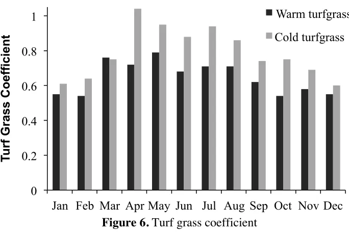
inch = 0.624 gpsf. Household agents can use one of two types of turf grass, warm and cold, and
monthly crop coefficients (Kcrop) are shown in Table 2 and Fig. 6 for each type of turf grass.
Table 2. Turf grass coefficients
Month Warm crop Cold crop
Jan 0.55 0.61
Feb 0.54 0.64
Mar 0.76 0.75
Apr 0.72 1.04
May 0.79 0.95
Jun 0.68 0.88
Jul 0.71 0.94
Aug 0.71 0.86
Sep 0.62 0.74
Oct 0.54 0.75
Nov 0.58 0.69
14
Figure 6. Turf grass coefficient
Agents are assigned a behavioral factor to represent how often they water their lawn (Fair and Safley 2013). Eqn. 4 is used to calculate the volume of water used for irrigation:
OWU =OIR TIR× (4)
where OWU is outdoor water use that is exerted by an agent (gpd), and OIR is outdoor irrigation
ratio, which represents the fraction of TIR that an agent uses to water the lawn (Table 3).
Table 3. Watering frequency distribution
Watering Frequency Outdoor irrigation ratio
Never water 0
Water new plants/stressed plants 0.5
Water regularly or in absence of rain 1
Household agents receive information from a water utility manager agent about the level of outdoor water use restrictions, based on drought stages. Each stage is characterized by the necessary restrictions, which must be implemented to preserve water supply. Households reduce outdoor demands based on utility restrictions.
Drought restrictions are typical management approaches that utilities across the U.S. use to alleviate demands in periods of water shortages or droughts. For the framework that is implemented here, the level of response, or reduction of demands, for household agents are calculated using the City of Raleigh’s Water Shortage Response Plan (City of Raleigh Public Utilities Department 2011). According to the report, per capita per day consumption goals are set
0 0.2 0.4 0.6 0.8 1
Jan Feb Mar Apr May Jun Jul Aug Sep Oct Nov Dec
Tu
rf
G
ra
ss
C
o
effi
ci
en
t
Warm turfgrass
15
for each conservation stage, and consumers should reduce their normal consumption to that amount. The agent-based modeling approach simulates that each agent reduces its use by the percentage specified after a drought stage is enacted (Table 4). For example, for Stage 2,
residents should reduce their normal demand of 65 gallons per day to 35 gallons per day, and the reduction is 54%. Indoor end uses are not affected by restrictions.
Table 4. Drought stages and level of response
Drought Stage Consumption Goal
(gpcpd)
Level of Response (Outdoor Restrictions) Permanent
Conservation Measures (PCM)
65 No restrictions
Advisory Stage 60 Reduce water usage by 10%
Stage 1 55 Reduce water usage by 17%
Stage 2 35 Reduce water usage by 54%
Stage 3 25 Reduce water usage by 67%
3.1.2 Population growth model
Population growth is simulated by increasing the number of household agents in the population at each time step, or month. Data for population growth are available through the U.S. Census, and data about household sizes are available through specific utilities. The total increase in population for each decade is divided by the average size of household at each decade to obtain the total number of households. The total number of households is divided by 120, the number of months in a decade, to calculate the monthly number of household agents that are added in the model. Households are populated based on the household size distributions. The population increases linearly through each decade.
3.1.3 Water utility manager agent
The water utility manager is simulated as an agent that receives information about the surface water elevation from the reservoir model at each monthly time step. Based on the reservoir storage, the water utility manager agent defines the level of water restrictions: Permanent
Conservation Measures, Advisory Stage, and Drought Stages 1, 2, and 3. Restrictions are enacted in response to decreasing reservoir storage.
16
storage in the reservoir for water supply, or water supply storage pool (WSSP). Storages of less than 70%, less than 50%, less than 30%, and less than 10% correspond to triggers for the Advisory Stage, Stage 1, Stage 2, and Stage 3, respectively. The reverse triggers for Stage 1, Stage 2, and Stage 3 are 90%, 70%, and 50% of the reservoir storage, respectively. The drought stage triggers are shown in Table 5.
Table 5. Drought stages and triggers
Drought Stage Trigger
(% WSSP)
Reverse Trigger (% WSSP)
Permanent Conservation
Measures (PCM) N/A N/A
Advisory Stage < 70% N/A
Stage 1 < 50% >= 100%
Stage 2 < 30% >= 70%
Stage 3 < 10% >= 50%
3.1.4 Water reservoir model
Reservoir storage is calculated on a monthly time-step using the continuity equation:
1
t t t t t t
S =S− +I −R WS− −SP (5)
where St is the volume of water stored in the reservoir at time step t; It is the monthly net inflow
to the reservoir (inflow plus precipitation over the lake surface minus evaporation from the lake
surface). Rt is the reservoir outflow (water quality releases) at time step t. WSt is the total water
supply, which is the sum of the indoor and outdoor demands withdrawn from reservoir at time
step t, and SPt is reservoir spill, which is released when the water level within the reservoir
exceeds a pre-defined control elevation.
At the beginning of each month, the reservoir model receives stream flow values based on
17 3.2 MODEL EVALUATION
The model is evaluated to assess the accuracy in simulating the water supply system through a set of statistical criteria. Models are evaluated using three evaluation statistics, described as follows.
The absolute error is the magnitude of the difference between the exact value and the simulated value. The relative error is the absolute error divided by the magnitude of the exact value which
is expressed as a percentage. RE value is calculated:
(
)
1 1 (%) 100 n i i i n i i O S RE O = = ⎛ ⎞ − ⎜ ⎟ ⎜ ⎟ = × ⎜ ⎟ ⎜ ⎟ ⎝ ⎠∑
∑
(6)where n is number of observations, Oi is observed value at time i, and Si is the value simulated by
the model at time i. A smaller value of RE indicates better performance for the model.
Percent bias (PBIAS) measures the average tendency of the simulated data in exceeding or
under-estimated the observed data.
(
)
1 1 100 n i i i n i i O S PBIAS O = = ⎛ ⎞ − ⎜ ⎟ ⎜ ⎟ = × ⎜ ⎟ ⎜ ⎟ ⎝ ⎠∑
∑
(7) The optimal value for this criterion is zero, and low-magnitude values indicate accurate model simulation. Positive values indicate model underestimation bias, and negative values indicate model overestimation bias.The Nash-Sutcliffe efficiency (NSE) is a normalized statistic that determines the relative
magnitude of the residual variance compared to the observed data (Nash and Sutcliffe 1970).
NSE is computed as shown below:
(
)
(
)
2 1 2 1 1 n i i i n i O i O S NSE O M = = ⎡ ⎤ − ⎢ ⎥ ⎢ ⎥ = − ⎢ − ⎥ ⎢ ⎥ ⎣ ⎦∑
∑
(8)MO is the mean of observed data. NSE ranges between −∞ and 1.0 (1.0 inclusive), and NSE
18
as acceptable levels of performance. Values less than 0.0 indicate that the mean observed value is a better predictor than the simulated value, which indicates unacceptable performance.
3.3 SUSTAINABILITY INDEX
Alternative management policies are evaluated using a sustainability index (Sandoval-Solis et al. 2010). The analysis of a management policy focuses on system failure, defined as any output value in violation of a performance threshold. Probability-based performance criteria include reliability, which describes how often the system fails; resilience, which measures how quickly the system comes back to a satisfactory state once a failure has occurred; vulnerability, which indicates the significance of the likely consequences of failure; and maximum deficit.
3.3.1 Deficit
Demand (Demandt) is calculated at each time step as the total public water demand from the
reservoir, and Supply (Supplyt) is calculated as the volume of water that the reservoir can deliver
to the public. A deficit (Dt) is counted when the total water demand from reservoir is more than
the available storage in the reservoir; if the water demand is equal to water supply, deficit is zero
(Dt = 0). Therefore, when Dt is greater than zero, the system fails.
{
if Demand > Supply 0 if Demand = Supplyt t t t t t Demand Supplyt
D
−=
(9)
3.3.2 Reliability
Water demand reliability is the probability that the available water supply meets the water demand during the simulated period. A time-based reliability is used, which is calculated as the
fraction of time the water demand is fully supplied, or the number of times Dt = 0, with respect to
the number of time steps simulated (n months).
No. of times D 0
Rel t
n
= =
(10)
2.3.3 Resilience
Resilience is the capacity of a system to recover quickly from difficulties or period of failure and to adapt to changing conditions. As water supply is threatened due to climate conditions, which vary, resilience assesses the ability of water management policies to adapt to changing
conditions. Resilience is defined as the probability that a successful period follows a failure
period (the number of times that Dt = 0 follows Dt > 0) for all failure periods (the number of
19 No. of times D 0 follows D 0
Res
No. of times D 0 occurred
t t
t
= >
=
> (11)
3.3.4 Vulnerability
Vulnerability is the probable magnitude of deficits, if they occur (Hashimoto et al. 1982). Vulnerability expresses the severity of failures, because even when the probability of failure is small, the possible consequences of failure should be considered carefully. Vulnerability is the expected value of deficits, or the sum of the deficits divided by the number of deficit periods,
which is the number of times Dt > 0 occurs. Vulnerability is expressed as a dimensionless
number by dividing the average annual deficits by the average annual water demand.
0
No. of times D 0 occurred
Vul
Average Annual Water Demand t n t t t D = = ⎛ ⎞ ⎜ ⎟ ⎝ ⎠ > =
∑
(12)3.3.5 Maximum deficit
The worst-case annual deficit is the maximum deficit.
(
)
max Max def
Average Annual Water Demand
Annual
D
=
(13)
3.3.6 Sustainability index
Finally, the Sustainability Index (SI) represents the aggregate sustainability based on a
combination of the performance criteria described above, including the reliability, the resilience, the vulnerability, and the maximum deficit. The index is defined a geometric average of the performance criteria.
(
)
1/4Rel Res 1 Vul (1 Max def)
SI =⎡⎣ × × − × − ⎤⎦
20 4 RESULTS
4.1 Application of ABM framework for Raleigh, NC Water Supply
The agent-based modeling framework is applied to simulate the water supply system of Raleigh, North Carolina. The city of Raleigh has a population of approximately 486,000 inhabitants over an area of 142.8 square miles in 2013, and the population of Raleigh is projected to increase to 848,000 inhabitants by the year 2032, as reported by the U.S. Census. The primary water supply source for the city is Falls Lake, which is a man-made reservoir located on the upper Neuse River and managed by U.S. Army Corps of Engineers. The Raleigh Water Utility provides water to Raleigh and an additional six surrounding communities, Garner, Wake Forest, Rolesville, Knightdale, Wendell, and Zebulon. Due to the population growth in the city of Raleigh and surrounding communities served by Falls Lake over the last decade, the water storage in Falls Lake has been increasingly stressed. Droughts were recorded in the years 2002, 2005, and 2007 (Kurt et al. 2009).
4.1.1 Data for household agents
The agent-based model was initialized with a population of agents, where each agent represents one household. Household agents are assigned household size, or number of members, based on data available through U.S. Census and Raleigh Department of City Planning (2013) (Tables 6-8).
Table 6. Raleigh population projections Population
1983 170,415
1993 244,430
2003 366,599
2013 529,840
2023 686,723
2033 848,365
Table 7. Raleigh household average size (Raleigh Department of City Planning 2013) Average household size
1980 2.67
1990 2.56
2000 2.54
2010 2.55
2020 2.55
21
Table 8. Raleigh household size distribution (Raleigh Department of City Planning 2013)
HOUSEHOLD SIZE Percent of
population (%)
1-person household 32.8
2-person household 31.8
3-person household 15.5
4-person household 12
5-person household 4.9
6-person household 1.8
7-or-more-person household 1.2
Total households 100
Using information in Table 9, agents are initialized with the build year for houses. Around 60% of houses are built before 1999.
Table 9. Distribution of build years for houses in Raleigh (Raleigh Department of City Planning 2013)
2010 Housing Statistic Year Built
Housing, Median Year Built 1993
Built 1999 or Later 41.58%
Built 1995 to 1998 7.52%
Built 1990 to 1994 5.88%
Built 1980 to 1989 14.97%
Built 1970 to 1979 10.94%
Built 1960 to 1969 8.37%
Built 1950 to 1959 5.13%
Built 1940 to 1949 2.61%
Built 1939 or Earlier 3.01%
22
Table 10. Total land area for seven communities served by the City of Raleigh Water Utility (Raleigh Department of City Planning 2013)
Year Land area (acres)
1980 35308.80
1990 58496.00
2000 75968.00
2010 92294.40
2020 160703.17
2030 201121.07
2040 242414.03
2050 285457.37
2060 331259.02
Table 11. Raleigh land use allocation (Raleigh Department of City Planning 2013)
Land Use Percentage
Residential-Single Family 34.10%
Residential - Apartment, Condominium 4.90%
Residential - Townhouse, Multiplex 3.20%
Residential - Other 0.60%
Non-Residential 57.20%
TOTAL 100.00%
Table 12. Allocation of residential zoning areas in Raleigh (Raleigh Department of City Planning 2013)
Percent of Residential Zoning
Units/ac
Pervious Area
Rural Residential 6.44% 1.089 80%
Residential 2 2.60% 2 75%
Residential 4 53.11% 4 62%
Manufactured Home 1.05% 6 62%
Residential 6 20.71% 6 62%
Special Residential 6 0.83% 6 62%
Residential 10 11.81% 10 35%
Residential 15 1.67% 15 35%
Residential 20 1.50% 20 35%
Residential 30 0.18% 30 35%
23
Each agent is assigned a pervious area, which is calculated based on the Curve Number (Table 12). Pervious area is simulated as turf grass, and the size of the pervious area is calculated as follows.
HPA HA PP= × (15)
TRA HA
NH
=
(16)
TRA TA RP= × (17)
HPA is household pervious area, PP is percentage of pervious area based on residential zone
information in Table 12, HA is household area, TRA is total residential area, NH is number of
households, TA is residential area, and RP is percentage of land use that is allocated to types of
land use development, including single family, apartment/condominium, townhouse/multiplex, other, and non-residential (shown in Table 11).
As shown in Eqn. 4, each agent is assigned a value for OIR, the outdoor irrigation ratio, and
these values are extracted from results of a survey of North Carolina residents about their
lawn-watering habits (Fair and Safley 2013). Household agents are assigned a value for OIR based on
the data reported in Table 13. Based on results reported in the survey (Fair and Safley 2013), 60% of homes have warm turf grass, and 40% have cold turf grass.
Table 13. Watering frequency distribution
Watering Frequency Percent Outdoor irrigation ratio
Never water 30.16% 0
Water new plants/stressed plants 42.31% 0.5
Water regularly or in absence of rain 27.53% 1
4.1.2 Data for Falls Lake Reservoir
The Falls Lake reservoir provides Raleigh and its service area with water supply, which is reserved in the Water Supply Storage Pool (WSSP) of the reservoir. The reservoir has multiple purposes, and water is allocated for flood control, water quality, and sediment storage; leaving only 42.3%, or 45,000 acre-feet of storage in Falls Lake for the WSSP storage (Fig. 7).
At the end of each time step, the water utility manger agent observes the amount of total storage in the reservoir and implements water restrictions. The WSSP is calculated as:
(
)
0.423
24
where TS is total storage and SS is sedimentation storage, shown in Fig. 7.
Figure 7. Water allotments for Falls Lake in MSL (Mean Sea Level): flood storage, water Supply, water quality, and sediment storage. Figure based on data from the City of Raleigh
Public Utilities Department (2011).
This storage supplies a service area population of approximately 500,000 which includes the City of Raleigh and the Towns of Garner, Wake Forest, Rolesville, Knightdale, Wendell, and
Zebulon. Residential part comprises 56.6% of total demand of water supply for the Raleigh service area, so as total residential water demand is calculated through the indoor and outdoor models during simulation. Non-residential water demand is simulated as a non-adaptive value, and the total demand as:
Residential Demand 0.566
TotalDemand =
(19)
25
The City of Raleigh Public Utilities Department uses surface water from Falls Lake and from the Swift Creek Lake system (Lakes Benson and Wheeler) as source of drinking water. Falls Lake Reservoir which is located on the upper Neuse River and northwest of the City of Raleigh has a surface area of over 12,500 acres and can provide Raleigh with up to 100 mgd (peak day), 66.1 mgd (annual daily average) for the fifty-year reliable yield during the period of record. The smaller Swift Creek lake system has a peak withdrawal rate of 20 mgd (peak day), 11.2 mgd (annual daily average) for the fifty-year reliable yield during the period of record. So as they can provide total of 77.3 mgd (annual daily average) during the period of record, and Falls Lake provides 66.1 of that, the total percentage of 85.5% of the total demand is provided by the Falls Lake during the simulation. Because just Falls Lake is modeled as the surface water storage, 85.5% of all demands are withdrawn from storage.
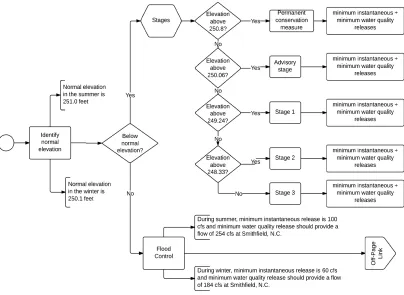
Water quality and flood control releases are simulated as the operational rules that control the release based on water level fluctuations in the reservoir on a daily basis and inflow projections for subsequent days (Figs. 8a and 8b). The overall plan of operation for water control of Falls Lake maintains a normal pool elevation of 250.1 feet M.S.L, November through March, and 251.0 feet M.S.L, May through September, with April and October as transition periods. Flood control storage space is reserved between elevations 250.1 and 264.0 feet M.S.L with surcharge storage provided above the crest of the free-overflow spillway (from elevation 264.0 feet M.S.L up to elevation 287.1 feet M.S.L). Conservation storage between elevations 250.1 and 236.5 feet M.S.L is reserved for water supply as well as low flow and water quality control. Immediately below the dam, a minimum instantaneous flow of approximately 60 cfs should be maintained November through March and 100 cfs April through October. Falls Lake also should be operated to maintain water quality flow requirements in the Neuse River at Smithfield Rive gage of 184 cfs and 254 cfs during the period of November through March and April through October, respectively. Flood control and water quality rules are detailed in the following sub-sections.
Operating Falls Lake for Flood Control
Storage of the 220,880 acre-feet between elevations 250.1 and 264.0 feet M.S.L is reserved exclusively for the detention storage of floodwaters. An additional 685,360 acre-feet of surcharge storage exists above the free-overflow spillway between elevations 264.0 and 287.1 feet M.S.L. The plan of operation of Falls Lake releases flows in a way that produce non-damage stages in the downstream reaches of the river whenever possible. The flood control objective is to store water in the flood control space in Falls Lake whenever the Clayton River gage exceeds damage flow of approximately 7,000 cfs. Because of the distance from the dam to Clayton and the amount of uncontrolled drainage area above Clayton, releases from the Falls Lake Dam may be terminated at the beginning of a storm to prevent normal discharges from contributing
26
capacity below Falls Lake is 4,000 to 8,000 CFS. Operational criteria for various flood situations are outlined as follows. Rules are summarized as follows and in Figs. 8a and 8b:
Lake elevation between 250.1 and 255.0 feet M.S.L.: if the flow from the uncontrolled drainage area above Clayton is, or is forecasted to be, equal to or greater than 7,000 CFS, the reservoir outflow will be the minimum instantaneous release of 60 CFS or 100 CFS. If the flow from the uncontrolled drainage area is less than 7,000 CFS, the reservoir release will be equal to the difference between 7,000 CFS and the flow from the uncontrolled drainage area, or 4,000 CFS, whichever is least.
Lake elevation between 255.0 and 258.0 feet M.S.L.: same as “a” except 4,000 CFS limitation is lifted.
Lake elevation between 258.0 and 264.0 feet M.S.L.: same as “b” except regulate to 8,000 CFS instead of 7,000 CFS at Clayton.
Lake elevation between spillway crest 264.0 and 268.0 feet M.S.L.: if the flow from the
uncontrolled drainage area above Clayton is, or is forecasted to be equal to or greater than 8,000 CFS, the only outflow from the reservoir will be from overflowing spillway until the peak flow at Clayton has occurred. After the peak at Clayton has occurred, releases from the conduit should be the maximum possible, which is 8,000 CFS.
Lake elevation above 268.0 feet M.S.L.: The conduit will be fully open to pass maximum discharge regardless of downstream flow conditions.
Operating Falls Lake for Water quality
27
28
Figure 8b. Water release operation rules flow chart, part 2.
4.1.3 Hydrologic data
29
Figure 9. Historical inflow to the reservoir
4.2 MODEL EVALUATION RESULTS
The agent-based model simulates monthly values for the total demands in the population, reservoir storage, and reservoir release. These values are compared to historical data for 1983-2013. Historical inputs are used to simulate the demands, total withdraws, release, and storage for Falls Lake. Outdoor demands are calculated (Fig. 10), and Fig. 11 shows the total water usage per capita per day for each month. Total demand decrease due to the effect of retrofitting indoor appliances.
Figure 10. Outdoor water demand per capita per day 0
200 400 600 800 1000 1200 1400
1983 1988 1993 1998 2003 2008 2013
Inflow (MSF)
0 50 100 150 200 250
1983 1987 1992 1997 2002 2007 2012
Outdoor demand (Gallon per capita
30
Figure 11. Total water demand per capita per day
Fig. 12 shows the total water withdrawal from Falls Lake reservoir for each month, which includes the residential and non-residential demands. The value for the observed water withdrawal from reservoir is plotted to compare with the simulated values. The model overestimates the demand, based on the observed data.
The observed data shows that, from 2007-2012, average demands in Raleigh decreased, potentially due to droughts and increases in water prices. To ensure the efficient use and protection of water resources, the city of Raleigh created a Water Shortage Response Plan (City of Raleigh Public Utilities Department 2011), as required by the North Carolina General Statute 143-355. The plan specified that reductions in water use should be enforced based on the
available water supply storage pool of Falls Lake, and specified reductions in non-essential water
use during times of water shortage, as described above. During the 2006-2007 drought, Falls
Lake dropped almost nine feet below its normal operating level, and the 450,000 consumers served by the Raleigh system cut their demands by 37% (Bowens 2007). Limited water use and watering restrictions, as specified in the plan, returned reservoir levels to normal elevations following the 2007-2008 drought. The decrease in water use, however, posed a serious revenue problem for the city of Raleigh, as customers sustained demand reductions beyond the prescribed period (Bracken 2009). In response, the city increased water rates and introduced a tiered rate structure in November 2010. The price schedule for residential water rates in Raleigh and Garner is as follows (City of Raleigh 2014).
Tier 1 = 0-4 hundred cubic feet per month (CCF) billed at $2.28 Tier 2 = 5-10 CCF billed at $3.80
Tier 3 = 11+ CCF billed at $5.07 0
50 100 150 200 250 300 350
1983 1987 1992 1997 2002 2007 2012
Total demand (Gallon per capita
31
Consumers continued to reduce demands, and total withdraws continued to decline after 2010-2011 (Fig. 12), perhaps in response to price changes. The ABM approach, however, captures reactions of consumers only as they decrease demands due to drought stages. The model does not represent the behaviors that consumers may have changed in response directly to droughts or to changes in the pricing structure. This is a limitation of the model that can be explored in further research.
Figure 12. Public water supply withdrawn from reservoir
Fig. 13 depicts the water quality releases of reservoir throughout the simulation period. The simulated and observed values are similar.
Figure 13. Reservoir release
The performance of the model in predicting reservoir storage is shown in Fig. 14. The model predicts reservoir release and storage well for the historic data. A spike in reservoir storage occurs in September 1999, however, which is not captured well by the model of reservoir storage. During the summer months of 1999, severe drought forced water restrictions across North Carolina. Hurricane Dennis made landfall in early September, and Hurricane Floyd, in mid-September. The combined effects from Dennis and Floyd led to record levels of
0 5 10 15 20 25
1983 1987 1992 1997 2002 2007 2012
Water Supply (acre-‐feet)
Th
ou
san
ds
Model Observed
0 50 100 150 200 250 300
1983 1987 1992 1997 2002 2007 2012
Release (acre-‐feet)
Th
ou
san
ds
32
precipitation and flooding throughout eastern North Carolina, and created flood conditions for Falls Lake. Parts of Wake County received nearly 20 inches of rain during September (State Climate Office of North Carolina 1999). The reservoir model can more accurately calculate water releases and storage during dry periods. During wet periods, the release is determined based on downstream flows, which are not accurately represented in the modeling framework. To better represent release during flooding conditions, the model can be extended to simulate routing throughout the Neuse River downstream of Falls Lake. The model is created to explore dynamics in drought conditions and can be improved to provide an effective tool for exploring reservoir operation and consumer reactions for flood management.
Figure 14. Reservoir storage
The ability of the model to simulate water supply, reservoir release, and reservoir storage are
evaluated using the statistical metrics, RE, PBIAS, and NSE (Table 14). The water release
simulation model shows accurate simulation, as demonstrated by low values of PBIAS, and NSE
equal to 0.7. Simulation of water supply is not acceptable based on the value for NSE, but the
relatively low value of PBIAS indicates that average tendency of the simulated data is not
significantly larger or smaller than the observed values. Overall, the reservoir storage is predicted with a relatively acceptable level of performance, based on the metrics.
Table 14. Model evaluation criteria
Criteria Storage
Simulation
Release Simulation
Water Supply Simulation
NSE 0.33 0.70 -0.19
PBIAS (%) 2.98% 0.03% -1.37%
RE (%) 13.69% 34.41% 20.63%
0 50 100 150 200 250 300 350
1983 1987 1992 1997 2002 2007 2012
Reservoir Storage (acre-‐feet)
Th
ou
san
ds
33
4.3 EVALUATING THE SUSTAINABILITY OF MANAGEMENT STRATEGIES FOR CLIMATE SCENARIOS
Future climate scenarios are constructed and used to evaluate the sustainability of six management scenarios. Future scenarios are simulated for 2013-2032 to explore the effectiveness of policies.
To simulate runoff process for the future time period three climate scenarios are defined, dry, medium, and wet climate. Scenarios are constructed by selecting 20 years of data from the historic 30 years. The dry scenario contains mostly years with below average values, the medium is around average, and wet is years with values mostly above average. Inflows to the reservoir, monthly precipitation, and monthly evapotranspiration are created for the three climate scenarios by sampling from the historic data (Figs. 15-17). The data records that were used for the three scenarios are shown in Table 15.
Table 15. Data used in creating Dry, Med, and Wet scenarios.
34
Figure 15. Future scenarios for inflow to the reservoir
Figure 16. Monthly average of precipitation for three climate scenarios 0
200 400 600 800 1000 1200 1400
2014 2016 2018 2020 2022 2024 2026 2028 2030 2032
Inflow (MSF)
DRY
MED
WET
0 1 2 3 4 5 6 7
Jan Feb Mar Apr May Jun Jul Aug Sep Oct Nov Dec
Precipita5on (Inch / Month)
35
Figure 17. Monthly average of evapotranspiration for three climate scenarios
Six management scenarios are defined by a set of rules for the actions of household agents and the utility agent. The first scenario is a base case, and household agents do not retrofit water appliances. All household agents water lawns using the demand calculated by Eqn. 3-6, without reductions due to lawn watering habits. The water utility manager agent does not enact drought stages. The second scenario is created to investigate the impact of retrofitting water appliances on residential water demand without any drought restrictions. Scenarios 3-6 analyze the impact of drought restrictions on sustainability by testing various settings for triggers (Table 16).
Table 16. Management scenarios
Scenarios Triggers
1 NO Retrofitting NO Drought Restriction NA
2 Retrofitting NO Drought Restriction NA
3 Retrofitting Drought Restriction 60%-40%-20%-0%
4 Retrofitting Drought Restriction 70%-50%-30%-10%
5 Retrofitting Drought Restriction 80%-60%-40%-20%
6 Retrofitting Drought Restriction 90%-70%-50%-30%
Management scenarios are analyzed for three defined climate scenarios. Indoor demands are not affected by drought restrictions and differ when household agents retrofit water appliances (Scenarios 2-6). Figs. 18 and 19 show average indoor demand for agents that do not retrofit and do retrofit appliances, respectively. Though households do not replace their water appliances with more efficient ones, the average demand decreases, because as more households with more water efficient appliances are added to the community of agents, they reduce the average indoor
0 1 2 3 4 5 6
Jan Feb Mar Apr May Jun Jul Aug Sep Oct Nov Dec
Evapotranspira 5on (Inch / Month)
36
demand (Fig. 18). Fig. 19 shows that each time step there is a small drop in demand, due to retrofits.
Figure 18. Indoor water demand per capita per day for Scenario 1. Agents do not retrofit water appliances.
Figure 19. Indoor water demand per capita per day for Scenarios 2-6. Agents retrofit water appliances.
Results for each management scenario and the dry climate scenario are shown in Figs. 20-24. Most notably, Scenario 6 shows that the water supply does not reach zero in any time step (Fig. 22). Because drought stages are enacted more quickly in response to decreasing reservoir levels,
0 10 20 30 40 50 60 70 80 90 100
1983 1987 1992 1997 2002 2007 2012 2017 2022 2027 2032 Indoor demand
(Gallon per capita per day)
0 10 20 30 40 50 60 70 80 90 100
1983 1987 1992 1997 2002 2007 2012 2017 2022 2027 2032 Indoor demand
37
water demands are reduced and the water supply is sustained. Therefore, water is available in the reservoir for subsequent time steps.
Figure 20. Outdoor demand for each management scenario and dry climate scenario Scenario 1
Scenario 2
Scenario 3
Scenario 4
Scenario 5
38
Figure 21. Total demand for each management scenario and dry climate scenario Scenario 1
Scenario 2
Scenario 3
Scenario 4
Scenario 5
39
Figure 22. Water supply for each management scenario and dry climate scenario Scenario 4
Scenario 5
Scenario 6 Scenario 1
Scenario 2
40
Figure 23. Reservoir release for each management scenario and dry climate scenario Scenario 4
Scenario 5
Scenario 6 Scenario 1
Scenario 2
41
Figure 24. Reservoir storage for each management scenario and dry climate scenario
The base case scenario overestimates residential water use, when compared to historic data and evaluated based on its sustainability index, which is around 40%. Fig. 25 shows the results for the six management scenarios. Results show that as retrofitting and drought restrictions are enacted, (1) maximum deficit decreases; (2) vulnerability decreases; (3) resilience increases; and (4) sustainability index increases. Scenario 2 demonstrates that retrofitting water appliances improves sustainability and all performance measures. Scenarios 5 and 6 improve the
sustainability index to nearly 80%, because the vulnerability and max deficit decreases due to the reactive triggers.
Scenario 4
Scenario 5
Scenario 6 Scenario 1
Scenario 2
42
Figure 25. Performance criteria and sustainability index values for management scenarios, dry climate scenario
For the med climate scenario, the sustainability index increases across the Scenarios (Fig. 26), through Scenario 6 increases the value of the index compared to Scenario 5 by a small value.
Figure 26. Performance criteria and sustainability index values for management scenarios, med climate scenario
For the wet scenario, there is little change in the value of the sustainability index or other metrics across the management scenarios (Fig. 27). For the wet climate, there is little stress on the reservoir and water supply system, and the performance criteria are at optimal values for all management scenarios.
0% 20% 40% 60% 80% 100%
1 2 3 4 5 6
Perfo
rma
nce Cri
teri
a &
Su st ai na bi lit
y
In
de
x
(%)
Scenarios
Reliability Resilience Vulnerability Max Deficit Sustainability Index
0% 20% 40% 60% 80% 100%
1 2 3 4 5 6
Perfo
rma
nce Cri
teri
a &
Su st ai na bi lit
y
In
de
x
(%)
Scenarios
43
Figure 27. Performance criteria and sustainability index values for management scenarios, wet climate scenario
0% 20% 40% 60% 80% 100%
1 2 3 4 5 6
Perfo
rma
nce Cri
teri
a &
Su
st
ai
na
bi
lit
y
In
de
x
(%)
Scenarios
44 5 DISCUSSION
This research demonstrates an approach to simulate behavioral factors for calculating water sustainability. The dynamic effects of reductions in outdoor water use to drought stage
restrictions, adoption of water-efficient appliances, and lawn watering habits are integrated in the modeling framework to develop a comprehensive simulation of the water supply-demand
balance. Data were collected from US Census, Raleigh Department of Urban Planning, City of Raleigh Water Utility, and a survey conducted about residential lawn water use, and data were synthesized within the modeling framework to simulate the actions and behaviors of local residents as accurately as possible.
Stochasticity is not represented in these results. Each model was executed for 30 random trials, but results show little variation due to little randomness in the model initialization. One source of stochasticity is in the calculation of the bath, leakage, and other end uses. Other parameters in the agent-based model are stochastic, such as the assignment of lawn watering behaviors.
Because the population is large, this stochasticity does not significantly affect the results. Water use behaviors can be more realistically represented in future research to better represent the inherent unpredictability in water use.
One outcome of this research is the application of agent-based modeling for simulating historic data. Few papers have tested and validated modeling for historic data (e.g., Galan et al. 2009). The model presented here is able to accurately simulate reservoir release and storage. A significant portion of the skill in this model comes from accurately capturing the reservoir release rules. Though some error remains in simulating the water consumption of residential users, the model captures trends in outdoor water use and reduction of demands due to increased efficiency in water appliances. The research conducted here explored a limited number of improvements to the model to gain accuracy. Additional investigations can explore assumptions and parameters used to calculate outdoor water use and habits.
45 6 SUMMARY AND CONCLUSIONS
This research develops an ABM framework to explore the dynamics of water supply and water demand in a water resources system. Dynamic interactions between consumers and water utility manager are simulated to evaluate conservation programs and drought restrictions. An
illustrative case study based on city of Raleigh, North Carolina, is used to test the methodology. The results demonstrate the influence of population growth, water use behaviors of consumers, water shortages, and management strategies on system-level performance of the reservoir storage. The model is able to more accurately simulate recorded data at Falls Lake when
behaviors representing retrofitting water appliances and lawn watering habits are included in the household agent simulation. Drought management strategies are simulated to explore the
performance of alternative strategies, based on the sustainability index. The results demonstrate that the framework can be used to assess alternative water management strategies, such as retrofitting appliances and water use restrictions.
46 7 RECOMMENDATIONS
The modeling framework that is developed here can be applied to provide insight for
management decisions. A few assumptions were made in the simulation that can be improved to provide results and analysis that will yield additional insight. Inflows to the reservoir were based on historical data, and not a hydrologic simulation model. To better capture the potential effects of alternative climate scenarios on the reservoir operations, a hydrologic model of the Falls Lake watershed can be coupled with the modeling framework and used to simulate expected
precipitation and temperature time series.
Additional water management scenarios can be included in the modeling framework in future work. For example, reclaimed and recycled water strategies may reduce the water supply demands. Other conservation measures include rainwater harvesting and localized water reuse technologies. These technologies may penetrate the market slowly through word-of-mouth and incentives provided by the utility. The dynamic adoption of the community can be simulated using an agent-based modeling approach. Finally, econometric models of water use can be developed to capture the effects of water pricing on water use and reservoir storage. New research can be conducted through collaborations with experts in social science and economy to further utilize the capabilities of the agent-based modeling approach to represent human
47 REFERENCES
Athanasiadis, I. N., Mentes, A. K., Mitkas, P. A., & Mylopoulos, Y. A. (2005). A hybrid agent-based model for estimating residential water demand. Simulation, 81(3), 175-187. Bharathy, G., & Silverman, B. (2012). Holistically evaluating agent-based social systems
models: a case study. Simulation: Transactions of the Society of Modeling and Simulation International, 89 (1), 102-135.
Bracken, David “City delays decision on water rate hike,” The News and Observer, [Raleigh,
NC] April 27, 2009,
http://www.newsobserver.com/2009/04/07/76078/city-delays-decision-on-water.html#storylink=misearch
Bowens, Dan “Falls Lake Reaches Record Low Level,” WRAL.com, [Raleigh, NC] November 20, 2007 http://www.wral.com/news/local/story/2070245/
City of Raleigh (2009) Designing a 21st Century City: The 2013 Comprehensive Plan for the City of Raleigh. Volume I: Comprehensive Plan.
City of Raleigh (2014) Utility Rates, Depositys, & Fees
http://www.raleighnc.gov/home/content/FinUtilityBilling/Articles/UtilityBillingDepositF ees.html, accessed July 29, 2014.
City of Raleigh Public Utilities Department (2011). City of Raleigh’s Water Shortage Response Plan.
DeOreo, W. B., Mayer, P. W., Martien, L., Hayden, M., Funk, A., Kramer-Duffield, & McNulty, A. (2011). California single-family water use efficiency study. Rep. Prepared for the California Dept. of Water Resources.
Edmonds, B., & Chattoe, E. (2005). When simple measures fail: characterising social networks using simulation. Social network analysis: advances and empirical applications forum. Oxford.
Fair, B. and C. Safley (2013). Residential landscape water use in 13 North Carolina communities. American Water Works Association, 105(10), E568.
Galán, J., del Olmo, R., & Lopez-Parades, A. (2008). Diffusion of Domestic Water Conservation Technologies in an ABM-GIS Integrated Model. Lecture Notes in Computer Science: Hybrid Artificial Intelligence Systems , 5271.
Galan, J., Loperz-Paredes, A., & Del Omo, R. (2009). An agent-based model for domestic water managemen in Valladolid metropolitan area. Water Resources Research , 45, 17 pg. Giacomoni, M., L. Kanta, and E.M. Zechman (2013). A Complex Adaptive Systems Approach
to Simulate the Sustainability of Water Resources and Urbanization. J. of Water Resources Planning and Management, 139(5), 554-564.
Gilbert, N. (2007). Agent-based models (quantitative applications in the social sciences). Thousand Oaks, CA: SAGE Publications.
Golembesky, K., A. Sankarasubramanian, and N. Devineni. (2009). Improved Drought Management of Falls Lake Reservoir: Role of Multimodel Streamflow Forecasts in Setting up Restrictions. Journal of Water Resources Planning and Management, 135(3), 188-197.