Atomic Scale Friction and Lubrication of Carbon Based Materials in Aqueous Environments.

ABSTRACT

LIU, ZIJIAN. Atomic Scale Friction and Lubrication of Carbon Based Materials in Aqueous Environments. (Under the direction of Professor Jacqueline Krim.)

The friction and wear properties of materials constitute a matter of great current interest, from both fundamental and applied points of view. They moreover impact a vast range of economic, environmental, and quality of life issues, as well as national security interests. This thesis reports on Quartz Crystal Microbalance studies that explore the fundamental atomic scale tribological properties of various carbon based materials in the presence of aqueous environments that range from direct immersion into water to exposure to increasing humidity.

Four topic of current interest have been studied: (1) The impact of surface charge on the nanotribological properties of nanodiamonds in aqueous suspensions, (2) The

Atomic Scale Friction and Lubrication of Carbon Based Materials in Aqueous Environments

by Zijian Liu

A dissertation submitted to the Graduate Faculty of North Carolina State University

in partial fulfillment of the requirements for the Degree of

Doctor of Philosophy Physics

Raleigh, North Carolina 2015

APPROVED BY:

_________________________ _________________________ Name of Committee Member Name of Committee Member

_________________________ _________________________ Name of Committee Member Name of Committee Member

____________________________ Name of Committee Member

ii

BIOGRAPHY

Zijian Liu was born to a loving family Changsha, Hunan Province of the People’s Republic of China. His father is an engineer and his mother is a doctor, the family

environment provided him a good study atmosphere and rose his interesting on science and technology.

After graduating High School with a lot of Chemistry knowledge learnt, he decided to study Physics at Nanjing University, NJU gave him a solid physics foundation and

encouragement to continue his research in physics in graduate studies.

iii

ACKNOWLEDGEMENTS

I would like to thank the many persons who helped me in my graduate studies. There are numerous persons…. My advisor, Jacqueline Krim, fellow students, family, and colleagues

iv

TABLE OF CONTENTS

LIST OF TABLES………...………..………..…..…x

LIST OF FIGURES………...………....xi

Chapter 1: Introduction………..……..……..1

1.1 Background……….………..…..…...1

1.2 Motivation for topic (1): Impact of surface charge on the nanotribological properties of nanodiamonds in aqueous suspensions………...3

1.3 Motivation for topic (2) Nanotribological properties of water films adsorbing atop, and absorbing below, graphene layers supported by metal substrates………5

1.4 Motivation for topic (3) Comparison studies of sliding friction levels water adsorbed on graphene versus graphene oxide substrates………..………...6

1.5 Motivation for topic (4): Comparison studies of the ability of water versus ethanol films to diffuse/slide through graphene oxide layers on porous alumina substrates…...8

1.6 Chapter 1 References………..……….…....10

Chapter 2: Theories of gas adsorption………...………..….12

2.1 Background………...………….……..….…..12

2.2 Thermodynamics and kinetics of adsorption………...……...…14

v

2.4 BET theory………..………..………..……...20

2.5 Adsorption on porous substrates………..…24

2.6 Surface potential………...………...27

2.7 Chapter 2 References………...…………...……...30

Chapter 3: Experimental technique and apparatus………...………...32

3.1 Introduction to QCM………..………..……...……...32

3.1.1 Mass loading of QCM and frequency shifts……….34

3.1.2 Quality factor and Energy dissipation………...……….……….39

3..1.3 Acoustic impendence and BVD circuits………...………....…...44

3.2 QCM measurements in liquid: Apparatus and data taking technique…………...…..53

3.3 Sample electrode preparation………..…………...……….55

3.3.1 Electrode preparation: Gold substrates ………...…………...…55

3.3.2 Electrode preparation: Aluminum substrates………...………..55

3.3.3 Electrode preparation: graphene transfer films on Aluminum substrates……...55

3.3.4 Electrode preparation: graphene/Ni (111) substrates..………...………56

3.3.5 Electrode preparation: graphene oxide films on Aluminum substrates …………..57

vi

3.3.7 Electrode preparation: graphene oxide films on porous Aluminum substrates…...60

3.4 Chapter 3 References………...………….…...61

Chapter 4: Tribological properties of nanodiamonds in aqueous suspensions: effect of the surface charge………...………..66

4.1. Introduction………..……...…...…….67

4.2 Materials and Methods ………...………...…...72

4.2.1 Materials………...……..….………..72

4.2.2 QCM electrode preparation………..…….……...74

4.2.3 QCM measurements………..…...………...75

4.2.4 QCM data analysis………...…....76

4.2.5 Dynamic Light Scattering (DLS) measurements………...………79

4.3. Results and discussion ……….………...79

4.3.1 Nanodiamond size and zeta potentials………...…....79

4.3.2 Tribological properties of nanodiamonds interacting with gold surfaces………...83

4.3.3 Macroscopic contact measurements………..…..85

4.4. Conclusions ………..………..……….………….87

vii

4.6 Chapter 4 References………..………...…………89

Chapter 5: Nanotribological properties of water films adsorbing atop, and absorbing below, graphene layers supported by metal substrates………..…..……….94

5.1 Introduction………..………..…....……94

5.2 Tribological properties of graphene in the presence of water………..…….95

5.3 QCM measurements of atomic scale friction………...….………...97

5.4 Experimental………..………..……..……..……..99

5.4.1 QCM Electrode preparation………..………...99

5.4.1a Aluminum electrodes………..…..…..…….…...99

5.4.1b graphene/Ni(111) electrodes……….………..…...…...99

5.4.1c Graphene transfer film electrode………...………..……100

5.4.2 Data collection method and apparatus………...………..…..……100

5.5 Results and analysis………...………..…….102

5.5.1 Water adsorption on aluminum………...……….……...…..102

5.5.2 Water adsorption on graphene/Ni(111)………...………..105

5.5.3 Water adsorption on transferred graphene………..……...106

viii

Chapter 6: Comparison studies of sliding friction levels water adsorbed on graphene and

graphene oxide substrates………...…...…....…….117

6.1 Introduction………..…………...……..….117

6.2 Tribological Properties of graphene oxide………...…119

6.3 QCM measurements of atomic scale friction………121

6.4 Experimental………..………..……122

6.4.1 QCM Electrode preparation………...………...122

6.4.1a Aluminium electrodes………...………..122

6.4.1b Electrode preparation: graphene oxide films on Aluminum substrates…………123

6.4.2 Data collection method and apparatus………...…123

6.5 Results and analysis………...…….125

6.5.1 Water adsorption on aluminum………...……..…125

6.5.2 Water adsorption on Graphene oxide………....134

6.6 Conculsion……….……...……….……136

6.7 Chagpter 6 references………...…...……..137

Chapter 7: Comparison studies of the ability of water versus ethanol films to diffuse/slide through graphene oxide layers on porous alumina substrates………...……...138

ix

7.2 Tribological Properties of graphene oxide………...……….………140

7.3 QCM measurements of atomic scale friction………....…………142

7.4 Experimental………..…..………..……..………144

7.4.1 QCM Electrode preparation………...………...…….…144

7.4.1a Aluminum electrodes………...……….…………...144

7.4.1b Electrode preparation: Porous Aluminum substrates………...………..…..144

7.4.1c Electrode preparation: graphene oxide films on porous Aluminum substrate….147 7.4.2 Data collection method and apparatus………...…………...….……147

7.5 Results and analysis………...………..…………..………….149

7.5.1 Water adsorption on aluminum………...……….……..149

7.5.2 Water adsorption on AAO samples………....162

7.6 Chapter 7 References………...……….…………..……..163

x

LIST OF TABLES

Table 3.1:BvD circuit Parameters for particular loads of AT-cut QCM………...……….48

Table 4.1. Properties of DND nanoparticles from the analysis of DLS data…………...….82

xi

LIST OF FIGURES

1.1 Schematic of positively and negatively charged nanodiamonds at the interface of a metal

immersed in water….……….………...………..4

1.2 Schematic of water adsorption on a graphene layer atop a metal substrate…....……..…...6

1.3 Water molecules have been reported to pass through graphene oxide films unimpeded…...7

1.4 Schematic of graphene oxide layers atop a porous alumina QCM electrode…………...8

2.1 Typical water isotherm BET plot for a flat Al QCM………...………..…..23

2.2 A Simulated adsorption isotherms for nitrogen adsorption on graphite surface coatings on a 5MHz QCM for a flat and porous substrate………...…………...25

2.3 Forward and reverse isotherms for water on a porous alumina electrode at T = 281K...26

2.4 Diagram of double layer and zeta potential………...27

3.1 Illustration of AT-cut QCM………...………..32

3.2 Lab use Quartz Crystal Microbalance setup schematic………...34

3.3 BvD equivalent circuit of a loaded quartz crystal in liquid……….…...44

3.4 Oscillation equivalent circuit in which a mass m is connected to an unmovable wall via spring with the spring constant k and a damping unit with the damping constant α…...49

xii

3.6 QCM measurements of gas uptake from the gas phase: Apparatus and data taking technique………..…...……….54

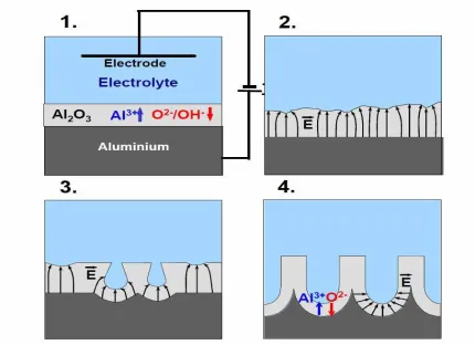
3.7 Schematic of the process employed to etch pores in aluminum to form porous alumina substrates. (image courtesy of A. Marek and A. Smirnov)………..…….….58

3.8 Scanning electron microscope images of typical porous alumina electrodes grown atop QCM’s. (mages courtesy of A. Marek and A. Smirnov.)………..…….…...59

4.1. A schematic illustration of the experimental QCM setup………..…………...70

4.2 Photograph of the QCM holder held horizontally with sixteen ball bearings loaded onto its surface electrode………...………....76

4.3 Size distributions of positively and negatively charge DND’s………..…………..80

4.4 Absolute values of the average zeta potential vs. average DND diameters for suspensions after ca. 2 yrs in storage……….………...81

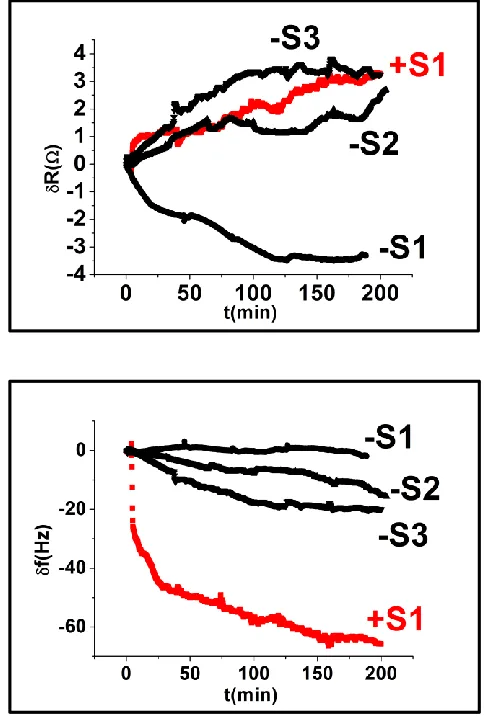
4.5 Characteristic mechanical resistance, Rm (top) and frequency shift, δf (bottom), vs. time, t, of a 5 MHz QCM with one gold electrode surface submersed in water and exposed to DNDs………...83

5.1 Water molecules approached to the surface. And Graphene “floating” on water molecules………..……...95

5.2 Schematic of the two samples studied……….………97

xiii

5.4 Water isotherm on bare Al QCM as a calibration………..……..………..103

5.5 Corrsepondece of 𝑑𝑅 and 𝛿(𝑄−1_{)………..……..……104}

5.6 Sliptime for water on Al surface versus reduced pressure………..……...105

5.7 frequency and amplitude response of water uptake on graphene/Ni(111). No slippage is detected……….…………..…...106

5.8 Characteristic change in frequency and resistance versus reduced pressure data sets for two differenct samples of one sided graphene……….108

5.9 Data from the upper figure of Fig. 5.8 superimposed with contributions from one side of the aluminum sample………..………110

5.10 BET analysis for two different samples of one sided graphene…………..……….112

5.11 Sliptime for water on graphene on QCM versus reduced pressure during the isotherm run for two samples………..114

6.1. Water molecules have been reported to pass through graphene oxide films unimpeded………..………..……..118

6.2 Schematic of the graphene oxide structure ………..…………...119

6.3 Schematic picture of water molucule travelling through nacre-like GO multilayers...121

6.4 Isotherm experiment setup………..………..124

xiv

6.6 Corrsepondece of 𝑑𝑅 and 𝛿(𝑄−1)………..……...………127

6.7 Sliptime for water on Al surface versus reduced pressure………..…...……128

6.8 Change in frequency and resistance versus reduced pressure during the isotherm run for two sample of graphene on QCM………...…………....130

6.9 Data from the upper figure of Fig. 6.8 superimposed with contributions from one side of the aluminum sample………..………..…..132

6.10 Sliptime for water on graphene on QCM versus reduced pressure during the isotherm run for two samples………..………...……….134

7.1. Schematic of graphene oxide layers atop a porous alumina QCM electrode: Water films traverse the films and fill the pores, while entrance to the pores by ethanol is blocked by the presence of the graphene oxide……….…………..………139

7.2 Schematic figure of (a)AAO modified QCM and (b)GO on top of AAO modified QCM………..142

7.3 Schematic of the process employed to etch pores in aluminum to form porous alumina substrates. (Image courtesy of A. Marek and A. Smirnov)………....145

7.4 Scanning electron microscope images of typical porous alumina electrodes grown atop QCM’s. (Images courtesy of A. Marek and A. Smirnov)……….…...146

7.5 Isotherm Experiment setup………..………...148

xv

7.7 Corrsepondece of 𝑑𝑅 and 𝛿(𝑄−1)………...……..………...…151

7.8 Sliptime for water on Al surface versus reduced pressure………..…………...…152

7.9 Change in frequency and resistance versus reduced pressure during the (a) Water and(b) ethanol isotherm on the AAO modified QCM………154

7.10 Change in frequency and resistance versus reduced pressure during the (a) Water and (b) ethanol isotherm of the GO/AAO modified QCM………...………...157

7. 11 BET analysis for (a)water and (b) ethanol isotherm of AAO modified QCM………...159

1 Chapter 1: Introduction

1.1 Background.

Tribology, the study of friction, lubrication and wear, constitutes an area of great current interest. Its impact is vast, spanning economic, environmental, and quality of life issues, not the least of which include national security and sustainability. [1, 2] The topic is growing in importance: As world population increases and demands on natural resources become strained, material waste levels and the massive energy losses associated with friction and wear that may once have been tolerated are no longer acceptable. The total frictional losses in a typical diesel engine, for example, exceed 10% of the total energy of combustion [2,3]. Achieving even a modest 1% reduction in such losses would save ~109 _{gallons of diesel fuel} in the U.S. alone – a significant savings from both economic and environmental viewpoints. Worldwide, the impact becomes even more massive, as building construction to house the world’s ever increasing population involves diesel driven machinery.

Technology is also getting smaller, with nanoscale and molecular assembly applications abounding. In these miniscule systems, the loss of a few molecules could lead to entire

system collapse; frictional heating could cause an entire nanoscale device to fail or evaporate. Trace contaminants are suddenly more prolific than the devices they are attaching to, and/or may diffuse from one region to another limited only by interfacial sliding friction effects. Such issues pose a major challenge to progress in applications that require precise knowledge and/or control of friction and wear in thin adsorbed films, including self-assembly and

2

graphene and carbon-based lubricants[7,8],and the stability of granular materials associated with frictional and frictionless contacts[9,10].

Carbon based materials, a mainstay of the lubrication industry, exhibit well-known sensitivities to the presence of water, in some cases very trace levels, in their surrounding environment [11]. Graphite, for example, is an excellent lubricant in air, but not vacuum: [12] It therefore fails for applications involving space exploration and satellites. Certain diamond-like carbons, meanwhile exhibit the opposite behavior, exhibiting low friction coefficients only in the absence of water. [13] But not all carbon based materials exhibit such sensitivities: The frictional behavior of graphene monolayers for example are reported to be insensitive to the presence of water. [14] Fundamental studies, particularly at atomic length and time scales, focusing on tribological properties of cabon-based materials in the presence of water, are required in order to understand the origin of such behaviors, which remain largely unexplained.

3

following sections. The results for the gas phase experiments (Topics 2-4) involve a detailed knowledge of theories of adsorptions phenomena, a topic that is described in Chapter 2. The experimental technique of QCM and apparatus employed for these studies are described in Chapter 3. The results of the four topics studied are presented in Chapters 4-7, followed by a summary and future outlook section in Chapter 8.

1.2 Motivation for topic (1): Impact of surface charge on the nanotribological properties of nanodiamonds in aqueous suspensions.

Present-day lubrication technologies were developed in an era that focused on wear elimination over friction energy losses with less attention paid to the environmental consequences. A variety of nanoparticulates are currently being actively pursued as

alternatives to these traditional oil-based lubricant additives. One emerging class of effective anti-friction and wear-preventing nanoparticulates consists of nanodiamonds obtained

mechanically (i.e., by crushing diamond crystals [15]) or through detonation of an oxygen-deficient mixture of explosives.[16] Crushed nanodiamonds are typically 100-500 nm in diameter and have potential as solid lubricants in vacuum [15] whereas the detonation nanodiamonds (DNDs) are much smaller, typically 4-7 nm in diameter, [16] with a narrow size distribution. Given that conventional additives to oil are insoluble or ineffective in aqueous environments, development of nanodiamonds as additives may ultimately allow for replacing centuries-old oil-based lubricating technologies.

4

mechanisms responsible for the macroscopic tribological performance is currently lacking in the literature. For the first topic studied, we examine the impact of the sign of the

nanodiamond’s surface charge on its tribological properties in aqueous solutions: Virtually

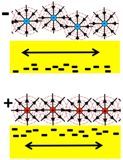
all dispersed nanoparticulates require surface charge to prevent coagulation and the eventual precipitation from a solution, but the role of the sign of the charge has heretofore been unexplored. The experiment is depicted schematically in Fig. 1.1.

Fig 1.1 Schematic of positively and negatively charged nanodiamonds at the interface of a metal immersed in water. The sign of nanodiamond surface charge is discovered to

5

As will be described in detail in Chapter 4, the tribological effects were observed to be highly sensitive to the sign of nanodiamond surface charge, at both nano and macroscopic lengthscales.

1.3 Motivation for topic (2) Nanotribological properties of water films adsorbing atop, and absorbing below, graphene layers supported by metal substrates.

Diffusion and sliding friction of water confined within or atop graphene and related materials is a matter of great current interest, with wide ranging applications that include filtration [6], energy conversion, nanofluids and desalination. Although the tribological properties of graphite, a common lubricant with known sensitivity to the presence of water, have been studied extensively at both macroscopic and microscopic length scales, it has been

6

Fig 1.2. Schematic of water adsorption on a graphene layer atop a metal substrate. Does water adsorb atop graphene layer or absorb below it?

As will be described in Chapter 5, the data indicate the presence of interstitial water increases sliding friction between the graphene and an aluminum substrate. In addition, although water layers condensed from the gas phase readily form below graphene layers transferred to aluminum substrates, they are observed to remain atop graphene/Ni(111) substrates and exhibit relatively high friction levels.

1.4 Motivation for topic (3) Comparison studies of sliding friction levels water adsorbed on graphene versus graphene oxide substrates.

Nair et al recently reported that the flow of water through graphene oxide laminate membranes is unimpeded[6], while the same membrane is leak tight to helium and other gases. Such “superlubric” behavior has also been reported in a variety of other graphene structures, for water. While numerous publications have reported “superlubric” behavior for

water in graphitic materials, they have stopped short of declaring water as exhibiting a truly zero friction flow, ie superfluidity. These include studies of water in carbon nanotube

7

measurements of sliding friction levels of water layers adsorbed on graphene oxide subtrates, to explore whether the sliding friction levels were in fact very low.

Fig. 1.3. Water molecules have been reported to pass through graphene oxide films unimpeded. Is the sliding friction of water on graphene water low or zero?

8

1.5 Motivation for topic (4): Comparison studies of the ability of water versus ethanol films to diffuse/slide through graphene oxide layers on porous alumina substrates.

As already mentioned, water adsorbed on graphene oxide substrates exhibits unique behavior. Nair et al , [6] in addition to reporting that the flow of water through graphene oxide laminate membranes is unimpeded, reported that the same membrane was impermeable to helium and other gases, including ethanol. What is the process of water travelling through the GO multilayers? To explore this in more detail, we studied water uptake on a QCM whose surface electrodes were formed from porous alumina covered by a graphene oxide layer (Fig. 1.4).

Fig 1.4. Schematic of graphene oxide layers atop a porous alumina QCM electrode: Water films traverse the films and fill the pores, while entrance to the pores by ethanol is blocked

9

10 1.6 Chapter 1 References

[1] H. P. Jost, Tribology & Lubrication Technology, 2005, 61, 18-22.

[2] K. Holmberg, P. Andersson and A. Erdemir, Tribology International, 2012, 47, 221-234.

[3] K. Holmberg, P. Andersson, N. O. Nylund, K. Makela and A. Erdemir, Tribology International, 2014, 78, 94-114.

[4] D. Speer, R. Eichhorn and P. Reimann, Phys. Rev. Lett. 102 #124101 (2009)

[5] Dan Wu and Shiqun Zhu, Phys. Rev. E 90, #012131 (2014)

[6] R. R. Nair, H. A. Wu, P. N. Jayaram, I.V. Grigorieva, and A.K. Geim, Science 335, 442 (2012)

[7] Chemistry and Technology of Lubricants, Third Edition, Springer-Verlag Berlin, Berlin, 2010.

[8] J. K. Lancaster and J.P. Pritchard, J. Phys. D: Appl. Phys. 14, 747(1981)

[9] R.P. Behringer, Comptes Rendus Phys. 16, 10 (2015)

[10] T. Shen, S. Papanikolaou, C. S. O’Hern and M.D. Shattuck, Phys. Rev. Lett. 113, #128302 (2014)

[11] J. K. Lancaster, Tribology International 23, 371-389 (1990)

11

[13] J.A. Heimberg, K.J. Wahl, I.L. Singer and A. Erdimer, Appl. Phys. Lett. 78, 2449 (2001)

[14] D. Berman et al., Materials Today 17, 31 (2014)

[15] A. V. Gubarevich, S. Usuba, Y. Kakudate, A. Tanaka and O. Odawara, Jpn. J. Appl. Phys. Part 2 - Lett. Express Lett., 2004, 43, L920-L923.

[16] N. R. Greiner, D. S. Phillips, J. D. Johnson and F. Volk, Nature, 1988, 333, 440-442.

12 Chapter 2: Overview of Sorption Theories

2.1 Background.

Sorption is defined as the physical and/or chemical process of one substance becoming attached to another substance. Sorption is classified into three categories, depending on the nature of the attachment:

1. Absorption: when particles (e.g. atoms, molecules or ions) enter the bulk phase (gas, liquid or solid phase)

2. Adsorption: in contrast to absorption, particles only attach to the surface of the bulk phase. This process therefore results in the creation of a film of the adsorbate on the surface of the adsorbent. It is a surface based process, while absorption results in a change to the whole volume.

3. Ion exchange: an exchange of ions between two electrolytes or an electrolyte. In this case both absorption and adsoption can take place simultaneously.

13

physisorbed, the electronic orbital patterns don’t change significantly for either the adsorbate

or the adsorbent species. So physisorption is also frequently referred to as van der Waals adsorption. There are some other differences between the two types of adsorption: Chemisorption usually requires a large activation energy, on the same magnitude as common chemical reactions. This is intuitive, as both related to breaking and rebuilding the covalence bonds. But for the process of physisorption, no activation energy is required. The energy of interaction between adsorbate and adsorbent particles are usually in similar magnitude of condensation. As for the reversibility, because the chemical nature of the adsorptive(s) may be altered by surface dissociation or reaction in such a way that on desorption the original species cannot be recovered; in this sense chemisorption may not be reversible. In contrast, if the van der Waals bonds broke in physisorption, the physical and chemical properties of both adsorbate and adsorbent would not change, so it is reversible. Also, in chemisorption, adsorbates will usually occupy certain adsorption sites on the surface to lower the energy of valence bonds, while in physisorption, under appropriate conditions of pressure and temperature, molecules from the gas phase can be adsorbed in excess of those in direct contact with the surface. Differences also in equilibrium states. In chemisorption, true equilibrium may be achieved slowly or even unreachable because of the large activation energy. In physisorption, equilibrium is readily established between the adsorbate and the fluid phase. Especially in solid/gas systems, at not too high pressures the extent of physical adsorption increases with increases in gas pressure and usually decreases with increasing temperature. In the case of systems showing hysteresis, the equilibrium may be metastable.

14

In physisorption, an image charge model is generally employed to estimate the electrostatic attraction and repulsion forces between adsorbate particles and adsorbent surface. In addition, the van der Waals binding energy can be analyzed by another simple physical picture: modeling the motion of an electron around its nucleus by a three-dimensional simple harmonic oscillator with a potential energy.

2.2 Thermodynamics and kinetics of adsorption

When studying adsorption, there are some general and basic questions that are of broad interest:

• How many particles can be adsorbed by a given amount of material? The thermodynamic

quantity of interest here is surface concentration.

• How does this amount depend on the state variables (temperature and pressure), i.e. how can

one control the adsorbate concentrate on by an appropriate choice of P and T?

• How can one determine the stationary and maximum adsorbed amount?

• Where are the adsorbed particles located at, on, and in the surface, respectively?

• How much energy is required to remove these particles from the surface, i.e., how strong are

the adsorptive bonds to the surface?

15

microscopic details or elementary processes on the atomic scale. It moreover incapable of predicting activation energies and, hence, provides hardly any information about kinetics (time dependences) of chemical reactions.

16

To quantify the thermodynamics during the adsorption process, the general method of Gibbs free energy equation is first utilized:

Δ𝐺_𝑎𝑑 = Δ𝐻_𝑎𝑑− 𝑇Δ𝑆_𝑎𝑑 (2.1)

Consider in the adsorption process, the parameters that might change during any change of state are temperature 𝑇, pressure 𝑃, surface area 𝐴, surface tension 𝜎, system volume 𝑉, chemical potential 𝜇, entropy 𝑆 and mole number of adsorbate species 𝑖. So if one takes the differential change of Gibbs energy, it can be presented as

𝑑𝐺 = (𝜕𝐺 𝜕𝑃)_𝑇,𝐴𝑑𝑃 + ( 𝜕𝐺 𝜕𝑇)_𝑃,𝐴𝑑𝑇 + ( 𝜕𝐺 𝜕𝐴)_𝑃,𝑇𝑑𝐴 + ( 𝜕𝐺

𝜕𝑛𝑖)_{𝑇,𝑃,𝐴}𝑑𝑛𝑖 (2.2)

Note by definition we have

(𝜕𝐺

𝜕𝑃)_𝑇,𝐴 = 𝑉 (2.3a)

(𝜕𝐺

𝜕𝑇)_𝑃,𝐴 = −𝑆 (2.3b)

(𝜕𝐺

𝜕𝐴)_𝑃,𝑇 = 𝜎 (2.3c)

So 𝑑𝐺 can be written as

𝑑𝐺 = 𝑉𝑑𝑃 − 𝑆𝑑𝑇 + 𝜎𝑑𝐴 + ∑ 𝜇𝑖 𝑖𝑑𝑛𝑖 (2.4)

From inspection of Eq. (2.4) it is apparent that the third term is decisive when the surface area/bulk volume ratio is large.

17

Γ = 𝑛𝑎𝑑

𝐴 (2.5) which is usually expressed in units of moles per unit area. Since gas adsorption is both pressure and temperature dependent, a common way to describe the equilibrium is to equate the chemical potential 𝜇 of adsorbate and gas phase:

𝜇𝑎𝑑 = 𝜇𝑔𝑎𝑠 and 𝑑𝜇𝑎𝑑 = 𝑑𝜇𝑔𝑎𝑠 (2.6)

In the Gibbs energy system, 𝜇 can therefore be presented as:

𝜇_𝑖 = (𝜕𝐺

𝜕𝑛𝑖)_{𝑇,𝑃,𝑗,𝑘…..(𝑜𝑡ℎ𝑒𝑟 𝑚𝑜𝑙𝑒 𝑛𝑢𝑚𝑏𝑒𝑟𝑠)} , (2.7)

which constitutes the basis for thermodynamic treatments of adsorption phenomena.

2.3 Langmuir Adsorption Isotherms

Adsorption isotherms provide a very useful experiment technique to measure the surface area and porosity of complex surfaces, and there are a variety of theories and analysis methods to interpret the adsorption isotherm results, including Linear isotherm[4], Freundlich isotherm[5], Langmuir isotherm [6], Kisliuk isotherm[7], adsorption enthalpy[8] and, the one to be commonly employed in this thesis, the BET theory[9]. The BET theory will be discussed after an overview of the Langmuir isotherm [6] , one of the earliest and simplest models for the form of an adsorption isotherm.

18

are mutually nonintereacting , and (4) no more than one molecule may reside at a given site [10, 11]. The last assumption is particularly problematic, as it requires that the first monolayer is complete before any particles are allowed to occupy the second layer. Under these assumptions, the adsorption process can be treated as a reaction where a gas molecule 𝐴_𝑔 reacts

with an empty site 𝑆, to yield an adsorbed complex 𝐴_𝑎𝑑:

𝐴𝑔 + 𝑆 ⇌ 𝐴𝑎𝑑 (2.8)

In the original derivation, first the rate of adsorption 𝑟_𝑎𝑑 and rate of desorption 𝑟_𝑑 is considered as

𝑟𝑎𝑑 = 𝑘𝑎𝑑𝑃𝐴[𝑆] (2.9)

𝑟𝑑 = 𝑘𝑑[𝐴𝑎𝑑] (2.10)

where 𝑃_𝐴 is the partial pressure of species A on the surface, [𝑆] is the concentration of bare sites per unit area, [𝐴_𝑎𝑑] is the surface concentration of A pre unit area, 𝑘_𝑎𝑑 and 𝑘_𝑑 are adsorption and desorption constant respectively.

At equilibrium the two rates equal to each other, 𝑘𝑎𝑑𝑃𝐴[𝑆] = 𝑘𝑑[𝐴𝑎𝑑], after rearrangement:

[𝐴𝑎𝑑]

𝑃𝐴[𝑆] =

𝑘𝑎𝑑

𝑘𝑑 = 𝐾𝑒𝑞𝑢

𝐴 _(2.11)

If it is a single adsorbate case, the sites need to be balanced as

[𝑆] = [𝑆₀] − [𝐴_𝑎𝑑] (2.12)

Where [𝑆₀] = 𝑆0

19 [𝐴𝑎𝑑]

𝑃𝐴𝐾𝑒𝑞𝑢𝐴 + [𝐴𝑎𝑑] = [𝑆0

] (2.13)

A new parameter 𝜃𝐴 can therefore be defined, as the fraction of the surface sites covered by molecules A:

𝜃_𝐴 = [𝐴𝑎𝑑]

[𝑆0] (2.14)

Substituting [𝑆₀] and [𝐴_𝑎𝑑] yields

𝜃_𝐴 = 𝑃𝐴𝐾𝑒𝑞𝑢𝐴

1+𝑃𝐴𝐾𝑒𝑞𝑢𝐴 (2.15)

The equilibrium constant 𝐾𝑒𝑞𝑢𝐴 can then be predicted in theory by

𝐾_𝑒𝑞𝑢𝐴 = 1

𝑃𝑟𝑒

−Δ𝐺𝑎𝑑/𝑅𝑇 ₌ 1

𝑃𝑟𝑒

−Δ𝑆𝑎𝑑/𝑅 _𝑒−Δ𝐻𝑎𝑑/𝑅𝑇 _(2.16)

where Δ𝐺_𝑎𝑑 , Δ𝑆_𝑎𝑑 and Δ𝐻_𝑎𝑑 are the equilibrium free energy, entropy and enthalpy of adsorption respectively.

If there are more than one species are present in the gas phase, the multiple adsorptions will happen together and compete with each other: Assuming all sites are equivalent to both A and B, and each site can only hold one molecule, for example two molecules A and B, their equilibrium constant can be presented as

[𝐴𝑎𝑑]

𝑃𝐴[𝑆] = 𝐾𝑒𝑞𝑢

𝐴 _(2.17)

and

[𝐵𝑎𝑑]

𝑃𝐵[𝑆]= 𝐾𝑒𝑞𝑢

20 Also all the sites are shared by both A and B so that

[𝑆] = [𝑆₀] − ([𝐴_𝑎𝑑] + [𝐵_𝑎𝑑]) (2.19)

So the coverage for A and B, 𝜃_𝐴and 𝜃_𝐵 can be written as

𝜃𝐴 =

𝑃𝐴𝐾𝑒𝑞𝑢𝐴

1+𝑃𝐴𝐾𝑒𝑞𝑢𝐴 +𝑃𝐵𝐾𝑒𝑞𝑢𝐵

(2.20)

𝜃_𝐵 = 𝑃𝐵𝐾𝑒𝑞𝑢𝐵

1+𝑃𝐴𝐾𝑒𝑞𝑢𝐴 +𝑃𝐵𝐾𝑒𝑞𝑢𝐵 (2.21)

2.4 BET theory

In actual experimental conditions, the Langmuir theory has many problems: These include the fact that the adsorption process is not uniform but is in fact random, the sites are not equivalent and most importantly: in most of cases adsorption will form multilayers in some locations on the surface in advance of the full monolayer completion.

To improve and develop the over-simplified Langmuir model, many different modifications have been suggested. Among them the BET theory is widely used model, and will be used in this work to estimate the surface areas of the substrates employed. It was first introduced in 1938 by Stephen Brunauer, Paul Hugh Emmett, and Edward Teller [6], developed for the case of multilayer adsorption. The BET theory is based on the following assumptions: [7]

1. Adsorption occur only on well-defined substrate sites (one per molecule)

21

3. The uppermost molecule layer is in equilibrium with the gas phase, i.e. similar molecule adsorption and desorption rates.

4. The desorption is a kinetically-limited process, i.e. a heat of adsorption must be provided:

(1) these phenomenon are homogeneous, i.e. same heat of adsorption for a given molecule layer.

(2) it is 𝐸₁ for the first layer, i.e. the heat of adsorption at the solid sample surface

(3) the other layers are assumed similar and can be represented as condensed species, i.e. liquid state. Hence, the heat of adsorption is 𝐸𝐿 is equal to the heat of liquefaction.

5. At the saturation pressure, the molecule layer number tends to infinity (i.e. equivalent to the sample being surrounded by a liquid phase)

After applying these assumptions to equilibrium status that the evaporation rate equals the condensation rate, and after some steps of derivation, the BET theory arrives at a straightforward equation:

𝑝 𝑣(𝑝0−𝑝)=

1 𝑣𝑚𝑐+

𝑐−1 𝑣𝑚𝑐

𝑝

𝑝0 (2.21)

Here 𝑝 is the equilibrium pressure at each point in the isotherm, 𝑝₀ is the saturated vapor pressure for this species, 𝑣 is the amount of gas adsorbed, 𝑣_𝑚is the volume of gas required to cover the surface with one complete monolayer of adsorbate. Note that 𝑣 and 𝑣𝑚 can be written in any units linear to the number of molecules, for example volume units and mass units. And

𝑐 is called BET constant, which proportional to exp (−𝐸1−𝐸𝐿

22

adsorption for the first layer and 𝐸𝐿 is the heat of liquefaction for second and higher layers, as

the they are assumed same value. 𝑅 is the gas constant and 𝑇 is the environment temperate.

In this equation, 𝑝 and 𝑝₀ can be read from the isotherm data, and 𝑣 can also be record using direct or indirect experiment techniques, and 𝑣_𝑚 and 𝑐 is the unknown terms, we especially interested in 𝑣𝑚 because once we know 𝑣𝑚 we can determine the structure and property of a certain surface.

So if one plots 𝑝

𝑣(𝑝0−𝑝) versus

𝑝

𝑝0 in the pressure region(0.05 <

𝑝

𝑝0< 0.35), it will be linear,

with slope

𝑐−1

𝑣𝑚𝑐, (2.22)

and intercept

1

𝑣𝑚𝑐 . (2.23)

This provides two equations in two unknowns, allowing one to solve for 𝑣𝑚 and 𝑐.

After 𝑣_𝑚 is determined, one can easily calculate the total surface area by apply the equation:

𝑆𝑡𝑜𝑡𝑎𝑙 = 𝑣𝑚𝑁𝑠

𝑉 (2.24)

Where 𝑁 is Avogadro's number, 𝑠 is the adsorption cross section of the adsorbing species, 𝑉

23

a monolayer on a perfectly flat and two-dimensional surface, to yield a value for the ratio of the actual surface area to that of a flat surface.

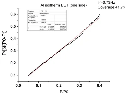
As an example, Fig.1 shows a typical BET plot for a water isotherm run one flat Al QCM . One monolayer of water adsorbed on a two dimensional substrate has mass per unit area of approximately 30 ng/cm2_{. The linear fitting is very well in the low pressure range, and the} interception slope can be determined easily as the table in . Fig.1

24 2.5 Adsorption on porous substrates

Several of the QCM samples studied in this research were rough or porous in nature. The nature of adsorption isotherms on such surfaces has been studied extensively in the literature for adsorption in general [12, 13] and uptake in particular on QCM surfaces electrodes with rough, fractal, or porous stuctures [14-16]. In such cases the form of an adsorption isotherm in the thick film (as opposed to the monolayer regime treated by the BET theory) is described by a combination of the form of the “Frenkel-Halsey-Hill” isotherm [15], derived under the

assumption that the film is a uniform slab of the bulk material, and that atoms interact via van der Waals forces, and the Kelvin equation [13] describing the pressure Pf at which cylindrical pores of radius r suddenly fill with the adsorbate condensing from the gas phase into a liquid state within the pores:

ln(Pf/P0) = (2 Vm cosγ)/(rRT) , (2.25)

rface tension of the liquid condensate, is the contact angle of the adsorbate with the surface, and P0 is the bulk vapor pressure of the liquid.

25

thus mass loading) are on the order of thousands of Hz, rather than tens of Hz, indicative of the deep pores employed for the studies.

Fig 2.2. From [14] Simulated adsorption isotherms for nitrogen adsorption on graphite surface coatings on a 5MHz QCM for a flat (dotted line) and porous (solid) substrate. The pores are cylindrical and identical with radius 2nm. One monolayer of liquid nitrogen on a flat surface (dotted line) corresponds to a frequency shift of 3.9 Hz. The porosity results in

26

Figure 2.3 Forward and reverse isotherms for water on a porous alumina electrode at T = 281K. (Reproduced from [16]) The resonant frequency of the QCM employed for this study was 5.25 MHz. Frequency shifts are on the order of thousands of Hz, rather than tens of Hz,

on account of the vastly increased surface area of the substrate.

Adsorption on surfaces that are neither perfectly flat nor a combination of perfectly flat plus uniform pores/cylinders can in many cases be described by a fractal geometry, whereby the adsorption isotherm is described by:

ln(P/P0) = - n); n = 3/(3-D) , (2.26)

27 2.6 Surface zeta potential

Fig 2.4 Diagram of double layer and zeta potential: Note that the zeta potential in this figure is negative, and the +y axis of the plot corresponds to increasingly negative potential[17].

28

It includes both anions and cations. When the particle is moving in solution, there is a plane called the slipping plane. Within the range of slipping plane, ions will move with the particle as a whole. The potential between the slipping plane and dispersion medium is called Zeta potential: It is a parameter that describe the electrokinetic potential of particle in colloidal dispersions[20].

The measurement of Zeta potential is measured by the electrophoresis phenomenon. When a charged particle moves when placed in an electric field, the particles with a zeta potential will migrate toward the electrode of opposite charge with a velocity proportional to the magnitude of the zeta potential. The velocity is proportional to electrophoretic mobility, which is a measurable parameter. This allows the zeta potential to be measured.

There is also an electric current or potential which originates when an electrolyte is driven by a pressure gradient through a channel or porous plug with charged walls. This potential is called the streaming potential. Practically, two reversible electrodes placed on either side of a fluidic geometry across which a known pressure difference is applied. When the electrodes are left floating, allowing a streaming potential to build up between the two ends of the channel. So that zeta potential can be calculated asU_str=(ϵ_r ϵ_0 ζ)/(ηK_L ) ΔP. Here η is dynamic viscosity of the liquid, K_L is specific conductivity of the bulk liquid[18].

29

30 2.7 Chapter 2 References

[1] Chemisorption and physisorption, IUPAC, 2001

[2] Gasser, R.P.H.; (1985) An introduction to chemisorption and catalysis by metals, Clarendon Press, Oxford

[3] Thermodynamics and Kinetics of Adsorption IMPRS-Lecture Series 2012: ‘Experimental and Theoretical Methods in Surface Science’ Klaus Christmann Institut für Chemie und

Biochemie, Freie Universität Berlin

[4] H. Yıldırım Erbil, "Surface Chemistry of Solid And Liquid Interfaces", Blackwell Publishing, 2006.

[5] Freundlich HMF. Über die Adsorption in Lösungen. Z Phys Chem. 1906;57(A):385–470

[6] Czepirski, L.; Balys, M. R.; Komorowska-Czepirska, E. (2000). "Some generalization of Langmuir adsorption isotherm". Internet Journal of Chemistry 3 (14).

[7] Kisliuk, P. (1957). "The sticking probabilities of gases chemisorbed on the surfaces of solids". Journal of Physics and Chemistry of Solids 3 (1–2): 95–101.

[8] Monk, Paul (2004). Physical Chemistry: Understanding our Chemical World. Wiley. p. 162.

[9] Brunauer, Stephen; Emmett, P. H.; Teller, Edward (1938). "Adsorption of Gases in Multimolecular Layers". Journal of the American Chemical Society 60 (2): 309–319.

31

[11] L. W. Bruch, Milton W. Cole and Eugene Zaremba(1997). Physical Adsorption: Forces and Phenomena. Oxford Science Publications

[12] Kenneth S.W Sing, Adsorption methods for the characterization of porous materials, Advances in Colloid and Interface Science, Volumes 76–77, 1 July 1998, Pages 3-11

[13] See, for example, R. Aveyard and D.A. Haydon, An Introduction to the Principles of Surface Chemistry, (Cambridge University, London, 1973)

[14] C.L. Wang, J. Krim and M. F. Toney, J. Vac. Sci. Tech. A 7, p 2481 (1989)

[15] P. Pfeifer, Y.J. Wu, M.W. Cole and J. Krim, Phys. Rev. Lett. 62, 1997 (1989)

[16] R. J. Lazarowich, P. Taborek, B.-Y Yoo and N.V. Myung, Jour. Appl. Phys. 101 art# 104909 (2007)

[17] Wikipedia-Zeta potential, https://en.wikipedia.org/wiki/Zeta_potential

[18] Lyklema, J. (1995). Fundamentals of Interface and Colloid Science. Academic Press.

[19] S. Xu and M.F. Arnsdorf, PNAS 92 (1995) 10384

32 Chapter 3: Experimental technique and apparatus

3.1 Introduction to QCM

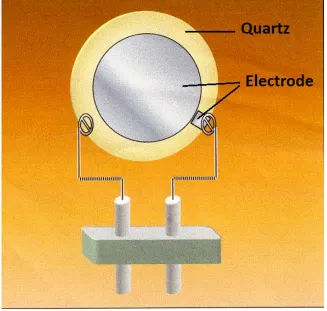
The Quartz Crystal Microbalance (QCM) has been used for decades to measure small mass adding or removal on a surface. Since quartz is piezoelectric, if an AC voltage is applied to quartz crystals cut at certain orientations, they will vibrate transversely with a characteristic frequency, in other words now the quartz crystals now become resonators [1]. There are many ways to cut quartz crystals, and each type of cut will result a different and unique vibrational mode when a voltage is applied. Among many kinds of QCM the most commonly used cut is the AT-cut, which has a so called thickness shear mode, as Fig. 3.1 shows. In practical situations, at this shear mode, the crystal is often made to have a frequency in the range of 1-30 MHz.

(a) (b)

Fig. 3.1 (a) an AT-cut QCM with no applied voltage (b) when voltage is applied on an AT- cut QCM, it will resonate[2].

33

more slowly [3,4]. The Q-factor for a 1MHz QCM is about 107, orders of magnitude better than the best LC circuits [5].The high Q-factor indicates that the QCM has a very low energy dissipation. Secondly, QCM has stable mechanical properties, its characteristic frequency is quite stable over short and long times, an essential feature for it to be used as a commercial unit and also lab tool. The third is its stability with respect to temperature variation, depending on the shape and orientation of the crystal is cut, many different modes of vibration can be used. It is possible to control and use the frequency-temperature characteristics of the QCM within close limits by an appropriate choice of cut [6].

34 3.1.1 Mass loading of QCM and frequency shifts

Fig. 3.2 Lab use Quartz Crystal Microbalance setup schematic

35

To be more quantitative, the shear resonate frequency of a QCM 𝑓0 depends on the properties of the quartz and also the thickness as equation 3.1 shows:

𝑓0 = √ 𝜇𝑞

𝜌𝑞/2𝑑𝑞 (3.1)

Where 𝜇_𝑞 = = 2.947 ∙ 1011 𝑔 · 𝑐𝑚−1· 𝑠−2 is the shear modulus (a ratio of sheer stress to

shear strain), 𝜌_𝑞 = 2.648 𝑔 ∙ 𝑐𝑚−3 _{is the density of quartz, and 𝑑}

𝑞 is the crystal thickness.

Since _√𝜇𝑞

𝜌𝑞 can be also presented as 𝜐 as shear-wave velocity so equation 3.1 can also be written

as equation 3.2[11]:

𝑓0 = 𝜐

2𝑑𝑞 (3.2)

Based on this, there is a linear relation between the frequency shift Δ𝑓 and the rigidly adsorbed mass Δ𝑚 as equation 3.3 shows:

Δ𝑓 𝑓0 = −

Δ𝑑 𝑑𝑞 = −

Δ𝑚

𝑀𝑞 (3.3)

Where 𝑀_𝑞 is the mass of quartz crystal [10], and the mass of the original quartz crystal 𝑀_𝑞 can

be presented as density multiple volume of quartz as equation 3.4

Δ𝑓 𝑓0 = −

Δ𝑚

𝜌𝑞(𝐴𝑑𝑞) (3.4)

Where 𝐴 is the surface are of the QCM. Replace 𝑑𝑞 with equation 3.1 and rearrange:

Δ𝑓 = − 2𝑓02

𝐴√𝜇𝑞𝜌𝑞 Δ𝑚 (3.5)Equation

36

for correlating changes in the oscillation frequency of a piezoelectric crystal with the mass deposited on one side it [12].

The advantage for Sauerbrey equation is, as for a known QCM, its 𝑓₀ and 𝐴 is a fixed number,

𝜇_𝑞 and 𝜌_𝑞are constants, so one can directly calculate the mass change on the surface from

measuring the frequency change of QCM, the negative sign means when Δ𝑚 is positive(adding on mass), the frequency will decrease. For example in our experiment, the most commonly used QCM is with 1 inch diameter and 5 MHz as its resonate frequency, so equation 3.5 is simplifies as

Δ𝑓 = −1.117 ∙ 107Hz ∙ 𝑔−1∗ Δ𝑚 (3.6)

Since the frequency can be measured up to 0.1 Hz easily, the minimum gas sensitivity is in the order of 10−9 _𝑔.

On the other hand, one can use the Sauerbrey equation to predict the frequency change for a known material thin film since Δ𝑚 can also be calculated by the density and volume of the material. It is an essential control method to have this theoretical prediction when performing a thin film deposition.

We note here the Sauerbrey equation is applied to only one side of the QCM has mass change, if mass is changing uniformly at both sides of the QCM, an coefficient of 2 must be add.

37

(2) the deposited mass must be distributed evenly and (3) the frequency changeΔ𝑓

𝑓0 < 0.02, i.e 105 Hz for a 5 MHz QCM.

If the change of the frequency is more than 2%, Sauerbrey equation must be extended to incorporate the elasticity of the deposition and the interaction between the add-on mass and the QCM must be considered. A method called Z-match was first introduced by Lu and Lewis[13,14] in 1972 tried to correlate mass change and frequency change in a more accurate way, as equation 3.7:

Δ𝑚 = 𝑁𝑞𝜌𝑞

𝜋𝑍(𝑓0+∆𝑓)∙ 𝑡𝑎𝑛

−1_{[𝑍 ∙ 𝑡𝑎𝑛 (𝜋}−∆𝑓

𝑓0 )] (3.7)

Where, the mass of change is still viewed as the thickness changing uniformly

Δ𝑚 is the change in mass per unit are in 𝑔 ∙ 𝑐𝑚−2

𝑁𝑞 is the Frequency Constant for AT-cut quartz crystal = 1.668 ∙ 1013 𝐻𝑧 ∙ Å

𝑍 is the Z-factor of film material = _√𝜇𝑞𝜌𝑞 𝜇𝑓𝜌𝑓

From the still relative simple equation, we can see the main factor that determine the relationship is the Z-factor, the accuracy of the mass load calculation is often limited by how well the Z-factor and density of the material are known. Density and Z- factor values are typically very close to bulk values [15].

38

In liquid, the response of the QCM is still extremely sensitive to mass changes at the QCM-liquid interface. Since than QCM has been used in direct contact with QCM-liquids and/or viscoelastic films for many years to assess changes in mass and viscoelastic properties during different surface processes.

When QCM is put in contact with a solution, there is a frequency decrease. As Nomura and Okuhara pointed out at first time, The frequency change of QCM (∆𝑓) depends on the liquid

density (𝜌_𝐿) and liquid viscosity (𝜂_𝐿). A quantitative understanding of the QCM behavior is a prerequisite for proper interpretation of experimental results when QCM is totally immersed in liquid. Glassford is the first trying to solve this problem[17], he discussed the liquid film deposition and liquid droplet deposition. Glassford and some other analyses are appropriate for thin films and partially elastic films but not for the case the total immersion of one surface of the crystal in a viscous liquid. Later on Kanazawa and Gordon improve the theoretic model and determined the behavior of the crystal/fluid system by examining the coupling of the elastic shear waves in the crystal to the viscous shear waves in the liquid. They proposed an equation to evaluate the frequency change of QCM immersion as equation 3.8[18]:

∆𝑓 = −𝑓₀3/2_√𝜌𝐿𝜂𝐿

𝜋𝜇𝑞𝜌𝑞 (3.8)

The derivation fo equation 3.8 is simply from Sauerbrey equation, as Sauerbrey can be write

as Δ𝑓 = − 2𝑓02

√𝜇𝑞𝜌𝑞 (

Δ𝑚

𝐴 ), in a Newtonian fluid the decay length, 𝑑, of an induced shear wave can be presented as

𝑑 = √_𝜋𝑓𝜂𝐿

39

If we assume that a region of fluid with a thickness of 𝑑/2 is coupled to the QCM, we can

substitute (Δ𝑚

𝐴 ) with 𝑑𝜌𝐿

2 , we have equation 3.8

Equation 3.8 is proved to be well predicting the frequency change for immersed QCM. For example, for a 1 inch diameter polished gold electrodes 5MHz crystal, when it was immersed in 20 ℃ pure ,we know 𝜌_𝐿 = 0.9982 𝑔 ∙ 𝑐𝑚−3 and 𝜂_𝐿 = 1.002 ∙ 10−2 𝑔 ∙ 𝑐𝑚−1∙ 𝑠−1_{,equation7 predicts a decrease in frequency of 715 Hz, excellent agreement between the}

frequency equation and the experimental results has been proved[19-21].

3.1.2 Quality factor and Energy dissipation

In addition to study the mass changes on QCM surface by measuring the frequency, we also care about when mass/film is adsorbed or desorbed, how energy changes, i.e. the dissipation factor (equivalent to the resonance bandwidth). It is often measured to help analysis.

40

As the original two definitions of the quality factor, one of these definitions is the frequency-to-bandwidth ratio of the resonator:

𝑄 = 𝑓0

∆𝑓 (3.10)

where 𝑓₀ is the resonant frequency, ∆𝑓 is the half-power bandwidth i.e. the bandwidth over which the power of vibration is greater than half the power at the resonant frequency.

Another common used definition for Q is the ratio of the energy stored in the oscillating resonator to the energy dissipated per cycle by damping processes:

𝑄 = 2𝜋 𝐸𝑛𝑒𝑟𝑔𝑦 𝑠𝑡𝑜𝑟𝑒𝑑 𝑝𝑒𝑟 𝑐𝑦𝑐𝑙𝑒

𝐸𝑛𝑒𝑟𝑔𝑦 𝑑𝑖𝑠𝑠𝑖𝑝𝑎𝑡𝑒𝑑 𝑝𝑒𝑟 𝑐𝑦𝑐𝑙𝑒 (3.11)

It can also linked with the resonate frequency as

𝑄 = 2𝜋𝑓₀𝐸𝑛𝑒𝑟𝑔𝑦 𝑠𝑡𝑜𝑟𝑒𝑑

𝑃𝑜𝑤𝑒𝑟 𝑙𝑜𝑠𝑠 (3.12)

The factor 2π makes Q expressible in simpler terms, involving only the coefficients of the

second-order differential equation describing most resonant systems, electrical or mechanical. In electrical systems, the stored energy is the sum of energies stored in lossless inductors and capacitors; the lost energy is the sum of the energies dissipated in resistors per cycle. In mechanical systems, the stored energy is the maximum possible stored energy, or the total energy, i.e. the sum of the potential and kinetic energies at some point in time; the lost energy is the work done by an external conservative force, per cycle, to maintain amplitude.

As we know in a RLC circuits, the Q-factor is:

𝑄_𝑒 = 1

𝑅√ 𝐿 𝐶=

𝜔0𝐿

41

where 𝑅, 𝐿 and 𝐶 are the resistance, inductance and capacitance of the tuned circuit, respectively.

As an analogy the QCM resonator’s Q-factor can be write as [10]:

𝑄_𝑚= 𝜔𝑀𝑚

𝑅𝑚 (3.14)

Where 𝑅_𝑚 is the “mechanical resistance” and 𝑀_𝑚 is mass added.

Above is the expression for a bare QCM, if mass is added to the oscillating QCM, the overall dissipation will change, when reflecting on quality factor, the total mechanic Q is calculated the same way as electrical Q:

1 𝑄=

1 𝑄𝑎𝑑𝑑+

1

𝑄𝑚 (3.15)

As we can tell from the equation, in most cases if more mass is added, the energy losses increases and Q factor decreases further. But in some case, the Q factor increases as mass added, for example Goyal and Tadigadapa claims that the Q factor was found to monotonically increase as more SWNTs were added to the QCM resonator [24].

To describe the energy dissipation in QCM more intuitively, a “dissipation factor” 𝐷 is suggested, it is proportional to the energy dissipation, defined as the inverse of the Q-factor

𝐷 = 1

42

In the practical study of QCM, the change of the dissipation δ (1

𝑄)level is more focus, in

different medium and context, δ (1

𝑄) has different means and expression, for example when consider a adsorbed film on QCM, the change of dissipation read as[10]

δ (1

𝑄) = 2𝑅

𝜔𝜌𝑞𝑑𝑞 (3.17)

Where R is the mechanical resistance, 𝜔 is the angular frequency, 𝜌_𝑞 the density of quartz and

𝑑_𝑞 the thickness of QCM , this is derived by the acoustic impedance which will be introduced

later.

When QCM is immersed in liquid, δ (1

𝑄) can be write as [18]

δ (1

𝑄) = 2√ 𝜌𝐿𝜂𝐿𝑓0

𝜋𝜌𝑞𝜇𝑞 (3.18)

Where 𝜌_𝐿 and 𝜂_𝐿 is the density and viscosity of the liquid.

And here we also have to notice that Q factor are affecting the noise of frequency data recording, as Vig and Walls have proposed an empirical relationship between the smallest level of noise generated by an oscillator in vacuum and the quality factor of the QCM, Q , for sampling times, τ , between 0.1 and 10 seconds, as equation 3.19 shows[25]

𝜎_𝑦(𝜏)_𝑚𝑖𝑛 = 1.0∗10−7

𝑄 (3.19)

Where σ_𝑦2_{(𝜏) is defined by Allan etc as the variance of two measurements 𝑦} 𝑘

̅̅̅ and 𝑦̅̅̅̅̅̅_𝑘+1[26]

σ_𝑦2(𝜏) = 1

2〈(𝑦̅̅̅̅̅̅ − 𝑦𝑘+1 ̅̅̅)𝑘

43

So 𝜎_𝑦(𝜏) is the typical deviation of them, specific to the frequency measurements here, the

Allan variance is used as a standard of stability measurement in the time domain. The oscillator detection limit, i.e. the smallest frequency deviation that can be detected in presence of noise is equal to:

Δ𝑓(𝜏) = 𝜎𝑦(𝜏) ∙ 𝑓0 (3.21)

On the other hand, they also indicate that the maximum quality factor achievable for quartz crystal manufactured in the best condition is inversely proportional to the frequency, for example for an AT-cut QCM, the product 𝑄_𝑚𝑎𝑥∙ 𝑓₀ is limited by equation 3.22

𝑄𝑚𝑎𝑥∙ 𝑓0 = 1.6 ∗ 1013 𝐻𝑧 (3.22)

Substitute 𝑄_𝑚𝑎𝑥 in equation 3.22 with equation 3.19, we can get the expression of the minimum noise, supposing that you can get the maximum Q , increases with frequency

𝜎_𝑦(𝜏)_𝑚𝑖𝑛 = 6 ∗ 10−21_{∙ 𝑓}

0 (3.23)

In this way, the oscillator detection limit will be [27]

Δ𝑓_𝑚𝑖𝑛= 6 ∗ 10−21_{∙ 𝑓}

02 (3.24)

Also for gas phase and adsorbed thin film, there is another important parameter to evaluate the dissipation level. Think about if the QCM substrate suddenly stops, the gas molecules or thin films will also stops oscillating, but not simultaneously with the QCM, the velocity (and therefore momentum) of molecules or films will fall exponentially to zero. The time constant

τ for this exponential decay will depend on the friction between the film and the substrate, and

44

film slips before stopping. And the slip time can be determined by Q factor and the resonate frequency of the QCM as equation 11 shows [10]:

𝛿 (1

𝑄) = 4𝜋𝜏𝛿𝑓 (3.25)

3.1.3Acoustic impendence and BVD circuits

As mentioned before, the QCM resonator is always compared with a RLC resonate circuits, based on this idea, all the mechanical resonator can be depicted as an equivalent circuit, so as the QCM system. As Fig. 3 shows, the Butterworth-van Dyke (BvD) equivalent circuit is first introduced by Martin, Granstaff and Frye in 1991, the BvD circuits represents mechanical interactions of the resonator with equivalent electrical circuit components[30].

Fig. 3.3 BvD equivalent circuit of a loaded quartz crystal in liquid [27]

45

BvD equivalent. In the electro-acoustic analogy, within which stresses (rather than forces) are mapped onto voltages. The ratio of stress and speed at the crystal surface is called load impedance, 𝑍𝐿. We can see from Fig.2 the upper branch is called “electrical branch” and the lower branch is called “acoustic branch”. Cp is the electrical (parallel) capacitance across the

electrodes. LQ1 is the motional inductance (proportional to the mass). CQ1 is the motional capacitance (inversely proportional to the stiffness) and RQ1 is the motional resistance (quantifying dissipative losses). LQ3 is the motional inductance for the loaded mass, which is also proportional to the loaded mass, and LQ2 and RQ2 are the same parameter for the liquid loading. LQ3, LQ2 and RQ2 add together is called ZL , it is the total load impedance.

For a unloaded QCM, its characteristic circuit elements of BvD circuit is known as constants which only depends on the QCM’s own properties. The quantitative of the parameters are given

by equation 3.26 below:

𝐶_𝑝= 𝜀𝑞𝐴0

𝑑𝑞 (3.26a)

𝐶𝑄1 = 8𝐶𝑝𝐾02

(𝑁𝜋)2 (3.26b)

𝐿𝑄1 = 1

𝜔02𝐶𝑄1 (3.26c)

𝑅_𝑄1 = (𝑁𝜋)2

8𝐶𝑝𝐾02

𝜂𝑞

𝜇𝑞 (3.26d)

The constants here: 𝜀𝑞 is the quartz permittivity, 𝐴0 is the active area of the QCM, 𝑑𝑞 is the

46

5, . . . 𝐾₀2 _{is the electromechanical coupling factor for quartz, 𝜂}

𝑞 is the effective quartz viscosity, and 𝜇𝑞 is the shear modulus[28].

Also there is another expression for 𝑅_𝑄1 as

𝑅𝑄1 = 𝜂𝑞

𝑐66𝐶𝑄1(

𝜔 𝜔0)

2

(3.27)

Here 𝜔₀ is the angular series resonant frequency for the unperturbed (no mass loading) QCM = 2𝜋𝑓₀, 𝑓₀ is the series resonant frequency in hertz, 𝜔 is the angular excitation frequency =

2𝜋𝑓. 𝑐66 is the quartz elastic constant[29]. Also 𝜔0 is given by [31]

𝜔₀ = 𝑁𝜋

𝑑𝑞√

𝜇𝑞

𝜌𝑞√1 −

8𝐾02

(𝑁𝜋)2 (3.28)

In the same way, the parameters for the loading mass have their own expressions:

𝐿_𝑄2 = 𝜔0𝐿𝑄1

𝑁𝜋 √ 2𝜌𝐿𝜂𝐿

𝜔𝑐66𝜌𝑞 (3.29a)

𝑅_𝑄2 = 𝜔0𝐿𝑄1

𝑁𝜋 √ 2𝜔𝜌𝐿𝜂𝐿

𝑐66𝜌𝑞 (3.29b)

Above are the conductance and resistance from the liquid load, we can see they not only depend on the density and viscosity of the liquid, also depend on the conductance of the QCM itself.

For the mass load:

𝐿_𝑄3 = 2𝜔0𝐿𝑄1𝜌𝑠

47

As mentioned before, the effect of limited mass attached to the QCM surface can be approximated as a thin rigid film between the QCM and liquid/vacuum/gas phase. Here 𝜌_𝑠 is the film’s areal mass density and 𝜌_𝑠 = 𝜌_𝑓𝑑_𝑓 as 𝜌_𝑓 and 𝑑_𝑓 are the 3-D density and thickness of

the film.

In this model, the QCM will fit the parameters and calculations over a range of frequencies near series resonance (2% off 𝑓₀). For the unperturbed QCM, 𝜌_𝑠 = 𝜌_𝐿𝜂_𝐿 = 0; equations 3.26 indicate that L_Q2 = R_Q2 = L_Q3 = 0. And Figure 3 reduces to the usual BvD equivalent circuit

for the unloaded QCM. As surmised by Beck et al., liquid loading causes an increase in both the motional inductance (contributed by 𝐿_𝑄2,) as well as resistance (contributed by 𝑅_𝑄2 with

𝑅𝑄2 = 𝜔𝐿𝑄2) (32). In contrast, mass loading increases only the motional inductance,

contributed by 𝐿_𝑄3.

In summary, we can reorganize this BvD equivalent circuits to be comprised of 3 parts an inductor (𝐿_𝑚), a resistor (𝑅_𝑚) and a capacitor (𝐶_𝑚), which arise from the inertia, damping and elastic stress terms, respectively. They are the combination of the parameters from QCM itself, liquid environment and mass loading. To explain them more detailly, 𝐿_𝑚 means oscillation inertial component, which is related to the dislocated mass during vibration; 𝑅_𝑚 represents oscillating energy dissipation into the structure onto which the crystal is mounted and into the medium, including both viscous solutions and viscoelastic films; 𝐶𝑚 suggests the stored energy in oscillation, which is related to crystal elasticity[9,36,37].

48

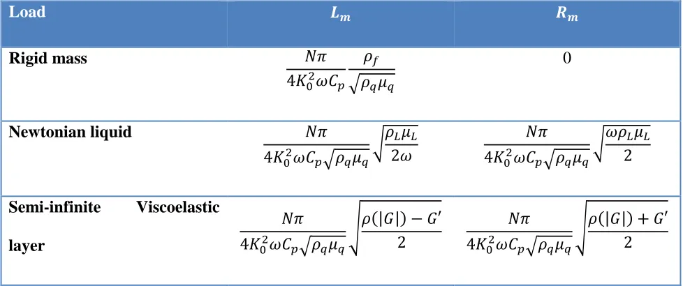
Table 3.1:BvD circuit Parameters for particular loads of AT-cut QCM

Load 𝑳_𝒎 𝑹_𝒎

Rigid mass 𝑁𝜋

4𝐾₀2𝜔𝐶_𝑝 𝜌_𝑓

√𝜌𝑞𝜇𝑞

0

Newtonian liquid 𝑁𝜋

4𝐾₀2_𝜔𝐶

𝑝√𝜌𝑞𝜇𝑞

√𝜌𝐿𝜇𝐿 2𝜔

𝑁𝜋 4𝐾₀2_𝜔𝐶

𝑝√𝜌𝑞𝜇𝑞

√𝜔𝜌𝐿𝜇𝐿 2

Semi-infinite Viscoelastic layer

𝑁𝜋 4𝐾₀2𝜔𝐶𝑝√𝜌𝑞𝜇𝑞

√𝜌(|𝐺|) − 𝐺′ 2

𝑁𝜋 4𝐾₀2𝜔𝐶𝑝√𝜌𝑞𝜇𝑞

√𝜌(|𝐺|) + 𝐺′ 2

Here G is the complex shear modulus of the viscoelastic material; the real part is the storage modulus G’ and the imaginary part is the loss modulus G’’.

As we can tell from equations 3.26, an interesting feature of the equivalent circuit model is that the elements that arise from mass and liquid loading are related to the unperturbed QCM parameters. Consequently, characterizing the unperturbed QCM fully determines the response to a given mass or liquid perturbation.

Also from equations 3.26, we can derive the BvD equivalent circuit expression for resonate frequency 𝑓0 and quality factor 𝑄 as

𝑓₀ = 1