Analysis of a Low Pressure UV reactor under Multiple Upstream Elbow Configurations using UV Sensitive Fluorescent Microspheres

(1)

ABSTRACT

ZHAO, XI. Analysis of a Low Pressure UV reactor under Multiple Upstream Elbow Configurations using UV Sensitive Fluorescent Microspheres. (Under the direction of Dr. Joel Ducoste.)

Upstream piping configuration has been known to impact the UV reactor validation using

biodosimetry tests. However, the influence of upstream configuration on the UV dose

distribution has not been experimentally investigated. This research was performed to

evaluate the UV reactor dose distribution under multiple upstream configurations using

UV sensitive fluorescent microspheres. The upstream hydraulics configurations included

two kinds of 90- degree bends and one straight pipe configuration. Experimental tests

were performed at 51 gpm flow rate, 91% UV transmittance (UVT) on a single lamp

low-pressure high-output (LPHO) UV reactor. The UV irradiation kinetics of the

photo-chemically active fluorescent microspheres was quantified with bench-scale

collimated beam experiments. The correlation with microspheres’ fluorescence intensity

distribution to UV fluence distribution was achieved by a statistical process involving

Bayesian and Markov chain Monte Carlo integration techniques. The results of this study

showed that the straight pipe configuration produced a shift in UV fluence distribution to

a higher UV fluence range compared to the two elbow configurations. No significant

difference was observed between the two elbow configurations. The fluorescent

microspheres Bayesian method can serve as an additional test to the traditional

biodosimetry for UV reactor validation and added confidence in the experimental results

(2)

Analysis of a Low Pressure UV reactor under Multiple Upstream Elbow

Configurations using UV Sensitive Fluorescent Microspheres

By

Xi Zhao

A thesis submitted to the Graduate Faculty of

North Carolina State University

in partial fulfillment of the

requirements for the Degree of

Master of Science

Civil Engineering

Raleigh, North Carolina

2007

APPROVED BY:

_________________________ _________________________

Dr. Detlef R.U. Knappe Dr. Francis de los Reyes

________________________________

(3)

BIOGRAPHY

Xi Zhao was born on June 19th, 1983 in Kunming, Yunnan, China. She is the only child

of Yonghua Zhao and Lin Sen. She spent 18 years in Kunming until she finished her high

school there. She graduated from Beijing University of Aeronautics and Astronautics in

July 2005 with a bachelor’s degree in Environmental Engineering. Right after her

graduation, she came to the United States in August 2005 to pursue her Master of Science

in Environmental Engineering with Department of Civil, Construction and Environmental

Engineering at North Carolina State University.

After graduate from North Carolina State University, she will work for Black & Veatch, a

worldwide civil and environmental consulting company, in Kansas City, MO as Civil

(4)

LIST OF TABLES

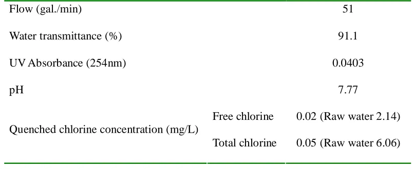
Table 1: Flow conditions and analyses of effluent water spiked with microspheres

for continuous-flows tests.………... 24

Table 2: Reduction equivalent fluence (REF) computed for MS-2, Bacillus Subtilis

and Cryptosporidium with fluence distributions results for three

configurations. The average UV fluence predicted by the Bayesian model (Fmean) was also compared... 25

Table 3: UV fluence distribution mean and standard deviation computed by

Bayesian model for the sensitivity test.……...………...…….. 26

Table 4: Mean and standard deviation of the experimental continuous-flow microspheres’ fluorescence distribution for the three upstream

(6)

LIST OF FIGURES

Figure 1: Photograph of LPHO UV reactor....……… 28

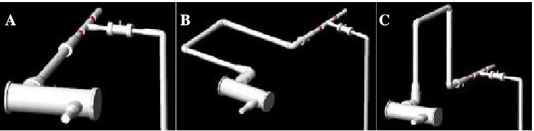
Figure 2: AutoCAD designs of three inlet configurations. A: Straight pipe configuration; B: 90 elbow horizontal configuration (Elbow 2); C: 90

elbow vertical configuration (Elbow 1)………... 29

Figure 3: Photograph of pilot test configurations... 30

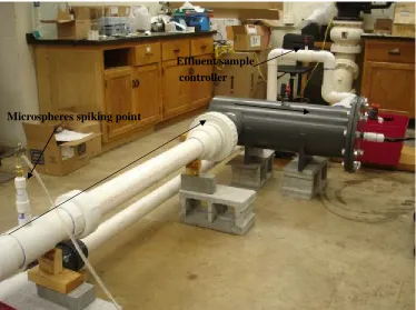
Figure 4: Photograph of pilot test that display injection and sampling points....…… 31

Figure 5: Photograph of Collimated beam apparatus.………....……. 32

Figure 6: QQ-plot for continues-flow microsphere fluorescence distribution data.... 33

Figure 7: Comparison of microspheres’ fluorescence intensity distribution for bench-scale collimated beam experiments at 0, 40 and 120 mJ/cm2

fluence level... 34

Figure 8: Mean and standard deviation of the fluorescence intensity distributions obtained from collimated beam experiments... 35

Figure 9: Measured microspheres’ fluorescence intensity distribution for pilot continues-flow experiment at flow rate of 51gpm with straight pipe

configuration inlet. Control is the influent dark sample... 36

Figure 10: Computed UV fluence distributions of continuous-flows experiments under three different inlet configurations: straight pipe (straight); vertical 90 elbow (elbow 1); horizontal 90 elbow (elbow 2). The mean of UV fluence distribution (Avg) and the standard deviation (Sd) of the respective distribution are illustrated…... 37

Figure 11: UV fluence-response kinetics for Cryptosporidium (Qian et al. 2004),

(7)

Introduction

Ultraviolet (UV) disinfection for drinking water and wastewater treatment is

increasingly becoming a popular disinfection treatment alternative since it can inactivate

chlorine resistant pathogenic microorganisms such as Cryptosporidium and Giardia

without forming regulated disinfection byproducts (DBPs) (USEPA 2006). Under the

Long Term 2 Enhanced Surface Water Treatment Rule (LT2ESWTR), UV disinfection is

one of the options for public water systems (PWSs) to further reduce microbial

contamination of drinking water (USEPA 2006). Currently, PWS must ensure the

required log inactivation credit through a dose monitoring program that has been

validated over a range of UV transmittances, flow rates, and UV intensities as mandated

by the Stage 2 Disinfectants and Disinfection Byproducts Rule (S2DBPR) (Wright and

Machey 2003).

UV reactors can be validated through on-site or off-site testing. Most equipment

manufactures choose off-site validation as the first option since a broader range of flows

and water quality conditions can be tested compared to limited on-site testing conditions

(Kelly et al. 2004). In order to effectively validate future UV installations, it is essential

for the off-site validation protocol to set up hydraulic configurations that cover the

possible on-site requirements. The flexibility required, however, for the piping gallery to

accommodate all possible treatment plant UV installations at validation facilities may be

too costly. For this reason, the US EPA’s Ultraviolet Disinfection Guidance Manual

(UVDGM) provides three recommendations for inlet and outlet piping configurations

(8)

hydraulic condition, which is assumed to be met by placing a single 90- degree bend, a

“T” bend, or an “S” bend upstream from the reactor inlet (USEPA 2006). However, the

validation of this “worst case” scenario has come under question by researchers who have

utilized computational fluid dynamics (CFD) models to simulate UV reactor

performances and showed that not all influent bend configurations lead to a reduction in

the log inactivation compared to the straight pipe configuration (Ducoste et al., 2005).

Limited studies have shown a reduction in the log inactivation when a single 90-degree or

T-bend has been placed upstream from a UV reactor compared to a straight pipe

configuration (Ducoste and Linden, 2006).

Photochemically active fluorescent microspheres as non-biological surrogates

have been investigated as a tool to measure the actual fluence distribution of a UV reactor

rather than biodosimetry and chemical actinometry that only provide a measure of the

average UV fluence. Previously, microspheres have been investigated as indicators for

pathogen inactivation in ozone reactors (Marinas et al. 1999), filtration experiments (Dai

and Hozalski 2003), and sequential disinfection processes with ozone and chlorine (Baeza

and Ducoste 2004). For UV disinfection, fluorescent microspheres were selected to use as

a photobleachable probe of UV fluence in a reactor (Anderson et al. 2003) but without

comparison to other conventional methods or modeling.

Dyed microspheres were used to measure the cumulative UV fluence distribution

together with such parallel methods as biodosimetry and numerical simulation to give a

comprehensive assessment of a UV reactor (Blatchley et al. 2006). While the cumulative

(9)

difficult to examine what individual UV fluence was impacted by the operational change.

A stochastic hierarchal process involving Bayesian statistics and the Markov chain Monte

Carlo integration technique was used to correlate the microspheres’ fluorescence intensity

distribution to the UV fluence distribution (Bohrerova et al. 2005). In Bohrerova et al.,

the results were compared with the fluence distribution predicted using a CFD model at

multiple flow rates. However, no designs on upstream configuration were performed by

any of these previous studies. The advantage of using dyed microspheres to assess the

impact of the upstream hydraulic configuration on the UV reactor performance is that it

provides more detailed information about changes in the fluence distribution compared to

just the average fluence. In addition, the direct quantification of the UV fluence

distribution using fluorescent microspheres measurement can help improve the validation

of CFD models, which is currently the only other approach for assessing the UV fluence

distribution.

The objective of this study was to provide insight into the impact of upstream

hydraulic configuration changes on the UV reactor performance with UV sensitive

fluorescent microspheres. A pilot-scale closed-vessel UV reactor housing a single

low-pressure high output (LPHO) mercury vapor lamp located at the reactor center line and

emitting principally at 254nm, was used for the test. Fluorescent microspheres were

injected into the main flow under three different upstream configurations that included a

(10)

Materials and Methods

UV Reactor

The reactor subjected to the validation test was a closed-vessel reactor, which was

made with a 12” diameter schedule 80 PVC pipe that is 3 ft long. Water flows through a

6” PVC pipe from one side of the reactor to another side and parallel to the lamp arc

(Figure 1). The reactor has only one LPHO UV germicidal lamp installed axially inside

the reactor center line. The LPHO UV lamp was operating at 87 Watts with 28 Watts UV

output at 254nm (catalog number 05-0264 GHO36T5/L/4PSE, Atlantic Ultraviolet Corp.)

Hydraulic Configurations

The UV reactor was tested with three inlet configurations to simulate different

approach hydraulic conditions. Configuration A was composed of a 4” diameter schedule

40 PVC pipe at a length of 40” (10 pipe diameters) to achieve the straight pipe hydraulic

condition. Configurations B and C were achieved using the same construction

components but oriented in different ways. As illustrated in Figure 2, configuration B was

equipped with 3 sections of 4” diameter schedule 40 PVC pipe at the length of 40”,

respectively. These three sections were connected by three 4” 90 bends and a 6” 90 bend

to allow final connection to the reactor. Configuration C was identical to configuration B

but installed at a right angle to configuration B. Configurations were connected to the

main pipe line by true unions, which made the switch between different configurations

(11)

In a previous study, a numerical simulation of a UV reactor with similar

inlet/outlet configurations showed that an upstream elbow configuration (configuration C)

may produce a higher log inactivation compared to the elbow configuration B or the

straight pipe configuration in Figure 2 (Ducoste et al., 2005). Although the model used in

Ducoste et al. (2005), was validated using experimental data for one of the elbow

conditions, no experimental biodosimetry tests were performed for the other

configurations. Moreover, none of the experimental tests in Ducoste et al. (2005), utilized

fluorescent microspheres to measure the fluence distribution.

Based on the CFD results in Ducoste et al. (2005), configuration B in the present

study is hypothesized to be the worst case scenario, which causes additional mixing and

possibly short-circuiting and a decrease UV disinfection performance. According to

Ducoste et al. (2005), configuration C is speculated to be the best case scenario. Ducoste

et al. (2005) hypothesized that configuration C will provide longer particle path lengths

due to the change in direction of the core fluid in the elbow away from the outlet and in a

rotating motion around the lamp. Due to this rotating motion, configuration C may result

in an increase UV disinfection performance compared to the straight pipe configuration.

Fluorescent Microspheres and Flow Cytometry

Experiments were performed using Fluorescent 14 polystyrene microspheres that

were obtained commercially from PolyMicrospheres, a Division of Vasmo, Inc.

(12)

emission maximum at 380 nm. The commercial microspheres were arrived from the

manufacturer stored in an aqueous solution of 0.2% solids content.

Flow cytometry was used to measure the fluorescence output of the microspheres.

The flow cytometer used in this study was a DakoCytomation MoFLo that included

Sortmaster, three lasers, and ten fluorescence detectors (DakoCytomation Ft. Collins,

Colorado), located at the Flow Cytometry and Cell Sorting Facility at North Carolina

State University College of Veterinary Medicine. A Coherent I90K Kryton tunable laser

was set to a wavelength of 350nm to individually detect fluorescent microspheres. The

fluorescence intensity emitted by each microsphere was detected by a photomultipler

detector after passing through a 405/30nm band-pass filter. Summit v4.3 (Dako Colorado,

Inc.) was used as the software platform for the flow cytometer and the results were

recorded on an arbitrary 405 MN linear scale of fluorescence intensity from 0 to 1023.

Each sample was used to obtain at least 10,000 microspheres to determine the

fluorescence distribution with gating applied to the boundary fluorescence to eliminate

background noise. Histogram results were extracted into txt. file by Summit v4.3 for

future analysis (Appendix A).

Pilot Test

Pilot system operation include an 11000 gallon storage tank filled with tap water,

a submersible pump that provides up to 108 gpm at 42ft head (Model 292 ½ H.P., Zoeller

Pump Co., Inc.), a turbine flow meter installed downstream of the pump with flow range

(13)

a 4L spiking dark container for mixing microspheres into the main water flow, a

peristaltic pump (7518-10, Masterflex L/S) for microspheres injection, several 3 inch

PVC ball valves to control the flow, a sample controller, and a test LPHO UV reactor.

The three inlet configurations were individually tested under identical conditions.

For each configuration test, the pilot was operated at 50 (±1) gpm, which provides a

theoretical residence time of 21s in the reactor. UV lamp was given 30 minutes to warm

up before each configuration test. After stabilization of the flow at 50 gpm, Microspheres

were spiked into the main flow at a rate of 0.5 gpm to provide a concentration of 1×105

microspheres mL-1. Effluent sample valve was set to full open at the commencement of

spiking the flow with microspheres. After three residence times (63 seconds) given to

ensure the reactor has reached steady state, a 1L sample was collected from the effluent

sample point.

2mL of 0.1 N sodium thiosulfate was added to the sample to quench any residual

free and combined chlorine. Preliminary bench scale experiments with the microspheres

in contact with the residual free and combined chlorine found in the tap water after two

hours showed no reduction in fluorescence. The quenching procedure was used as an

added level of quality control to eliminate any other possible source of fluorescence decay.

Once quenched, three 3 mL sub samples were collected and stored in 12×75 mm2 Falcon

(B.D. Lab Ware) tubes at 4 oC before analysis. Along with the reactor lamp turned on, a

dark test (i.e., lamp turned off) was conducted and effluent samples were collected for

bench-scale quasi-collimated beam experiments, water analyses, and for controls. The

(14)

Water Analyses

Absorbance at 254nm and pH were measured according to standard methods for

examination of water and wastewater (APHA 1992). Both influent and effluent dark test

samples were analyzed for free chlorine and total chlorine using the DPD Pocket

Colorimeteric Method, Hach Co. (Loveland, Co.) for both raw and quenched samples.

Quasi-Collimated Beam Settings

Bench-scale experiments were performed with the quasi-collimated beam

apparatus to provide the calibration curve for the microspheres’ fluorescence intensity

decay for known UV fluence values. The collimated beam, which contains 4 low pressure

(LP) UV mercury lamps, was calibrated by measuring the Petri dish factor, which

achieved a value of 0.96 (Bolton and Linden, 2003). Experiments were performed in

completely mixed Petri dishes with 15mL samples from the dark test effluent sample.

Samples were exposed to UV fluences of 5, 10, 15, 20, 30, 40, 60, 80, 100, and 120

mJ/cm2. UV fluence was calculated as the average irradiance multiplied by the exposure

time. The incident UV irradiance (mW/cm2) was measured at the surface center of the

liquid suspension by radiometer (UVX Digital radiometer E 27987/ UVP, Inc.). The

radiometer was calibrated with potassium iodide actinometry method (Rahn, 1997)

(Appendix B). The average UV irradiance was determined according to Bolton and

Linden (2003) as

(15)

Computation of the UV Fluence Distribution from Microspheres’ fluorescence

Intensity Measurements

In this study, the statistical approach developed by Bohrerova et al. (2005) was

used to compute UV fluence distribution from the microspheres’ fluorescence distribution.

A detailed discussion of this approach is provided in Bohrerova et al. (2005) and

summarized here. The UV fluence probability distribution function (UV-PDF) in the

reactor was determined using a Markov chain-Monte Carlo (MCMC) integration of the

Bayes theorem. The computed UV-PDF was based on the effluent measurements of

microspheres’ fluorescence of the continuous-flow tests and on measurements of the

fluorescence intensities decay of the microspheres’ fluorescence in the bench-scale

quasi-collimated beam experiments.

MCMC integration over the range of observed fluorescence distributions is an

important step to determine the corresponding fluence level distribution since a

fluorescence intensity distribution was generated for a known fluence level instead of a

single fluorescence value. As a result, the fluorescence distribution displayed overlaps

between each fluence level used in the calibration procedure with the collimated beam

apparatus. Therefore, a single fluorescence distribution can be attributed to a continuous

range of corresponding exposure fluences.

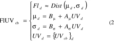
Two separate statistical models were built for the reactor results and the

bench-scale calibration results to resolve the unknown and known fluorescence distributions,

respectively. For the bench-scale experiments, the purpose was to determine the

(16)

UV fluence. Based on Bayes’ theorem, the statictical model can be shown as (Bohrerova

et al., 2005):

(

)

{

}











=

+

=

+

=

≈

=

d cb d d d d d d d d

UV

A

B

UV

A

B

Dist

Fl

σ σ µ µ

σ

µ

σ

µ

,

FlUV

_cb ₍₂₎

In Equation 2, FlUVcb is the UV fluences for the collimated beam experiments and

Fld is the microsphere fluorescence for a known single fluence level (UVd). Fld can be

characterized as either a normal or log normal distribution and is represented generically

by Dist(). According to Bohrerova et al. (2005), Fld was expressed as a Log-Normal

distribution due to the range and shape of the microsphere fluorescence distribution. On

the other hand, these distributions were described in the past as Gaussians (Anderson et al.

2003), and Weibull (Blatchley et al. 2006) distributions for different dyed microspheres.

In order to assess a better fluorescence distribution model for the specific microspheres

used in this research, the commonly used statistical technique quantile-quantile (QQ) plot

was investigated with Matlab to help determine which distribution best describes the

microspheres’ fluorescence data.

Figure 6 illustrates a representative QQ plot result for one of the continuous-flows

microsphere fluorescence distribution. The linear relationship between the normal

distribution theoretical quantiles and the experimental data quantiles suggests that the

microsphere fluorescence data can be charaterized under the normal distribution. Due to

the fluorescence results gating technique, which manually truncates the fluorescence

(17)

the very ends of the QQ plot did not follow the hypothetical linear line well. However, the

impact of those tail points was negligible since the majority population, which had

reached at least 10,000 obeservations, provided an R2 greater than 0.99 with the linear

relationship.

In Equation 2, a linear correlation was assumed between the averages (μ) and the standard deviations (σ) of the normal distribution for each fluence level tested in the collimated beam experiments. B μ, A μ, B σ, A σ was the set of fitting parameters from the

bench-scale collimated beam experiments statistical model. A μand A σwere the slopes of

the linear fit lines between UV fluences and the corresponding fluorescence average and

standard deviation, while B μ and B σwere the intercept of those two lines.

B μ, A μ, B σ and A σwere then used as the average and standard deviation values

for the reactor microsphere fluorescence data. Equation 3 displays the statistical model

used for the UV LPHO reactor fluorescence data (Bohrerova et al., 2005).

(

)











≈

+

=

+

=

≈

=

)

,

(

,

FlUV

_R

ρ

α

σ

µ

σ

µ

σ σ µ µ

Gamma

UV

A

B

UV

A

B

Dist

Fl

R R R R R R R R (3)

The UV fluence distribution in the reactor (UVR) was assumed to take the shape

of a Gamma distribution since it can produce a broad range of shapes that includes

log-normal and Weibull distributions. A review of the literature of studies that performed UV

reactor modeling showed that UV fluence distributions will have shapes consistent with

log-normal, Weibull, and Gamma distributions (Bohrerova et al., 2005; Ducoste and

(18)

Pareto distribution (with c1=1 and c2=5) and defines a decreasing distribution between c2

and ∞. The rate parameter (ρ) was assumed as an exponential distribution (with λ2=0.001). Exponential prior distributions were assigned to Bµ, Aµ, Bσ and Aσ with a decay rate of λ2, which defines it as a slowly decaying distribution between 0 and ∞.







=













)

(

)

,

(

2 2 1

λ

ρ

α

Exp

c

Pareto

(4)

As in Bohrerova et al. (2005), a range of c2 values were tested to explore its

sensitivity to the results and no difference was found beyond a value of 5. R. 2.5.0

statistical software was used to generate the best estimate for B μ, A μ, B σ, A σ and initial

data input for WINBUGS 1.4, which was used to generate the best estimates for α and ρ using MCMC integration. 1000 pairs of α and ρ, generated by WINBUGS, were resampled by R. 2.5.0 to generate the reactor UV fluence distribution based on the total of

200,000 values of UV fluence in the reactor (Appendix A).

Results and Discussions

Collimated-beam Results

Measurements of microspheres’ fluorescence intensity distribution for bench-scale

collimated beam experiments displayed a clear trend in the applied UV fluence. Figure 7

displays only three representative UV fluence levels to demonstrate the microspheres’

fluorescence reduction trend and the appearance of overlapping regions between the

distributions. Although each of the samples was exposed to a single fluence value,

(19)

heterogeneity among the microspheres’ size, shape, and surface characteristics (Blatchley

et al. 2006) as well as the amount of dye contained in each microsphere. Discussions with

fluorescence microspheres manufactures revealed that of these variables that impact the

fluorescence, the amount of dye contained on each microspheres is the most difficult to

control and would require more research into the dye application technique.

The linear relationship obtained from the mean of the fluorescence distributions

for collimated beam experiments (Figure 8) also illustrates that increasing the UV fluence

level will lead to a decrease in the microspheres’ fluorescence. The fluorescence intensity

decay rate constant was -1.76 cm2mJ-1, which was higher than -0.27 cm2mJ-1 found in

Bohrerova et al. (2005). The higher decay rate is likely due to the settings of the flow

cytometer that were different from Bohreroval et al. (2005) as well as differences in the

dye quantity with each microsphere used in the present study. However, the higher decay

rate constant has the added benefit of improving the results accuracy by indicating a

higher sensitivity and better separation between fluorescence distributions. Figure 8 also

displays the change in fluorescence standard deviation for each of the distributions. The

decay rate constant (-0.16 cm2mJ-1) indicates that the microspheres’ fluorescence

distribution had a broader variance for lower fluence level than that for the higher fluence.

A narrowing of the fluorescence distribution is expected with increasing UV fluence since

more of the dye is reaching the limit of zero fluorescence. Finally, the high R2 values

displayed in Figure 8 suggest that a linear relationship for the mean fluorescence and

standard deviation with the applied UV fluence is reasonable for the microspheres used in

(20)

Pilot Results

Figure 9 displays the control microspheres’ fluorescence intensity distribution

result along with the UV reactor data with the straight pipe inlet configuration at 51gpm.

The results in Figure 9 displays a significant reduction in the mean fluorescence intensity

along with a broader distribution for the straight pipe UV reactor data compared to the

control data (μreactor= 649, σreactor= 98, μcontrol= 801, σcontrol= 87). The broader variance was attributed to the microspheres exposure to a wide range of fluences that occurred from the

infinite number of paths that can be taken in the continuous-flow reactor. As discussed

earlier, the broad UV reactor fluorescence distribution tends to overlap with several

fluorescence distributions created at known fluence levels during the collimated beam

experiments. Consequently, the statistical models (Equations 2 and 3) were used to

resolve the UV reactor fluence distribution from the fluorescence distribution in Figure 9.

Figure 10 displays a comparison between the UV fluence distributions computed

by the Bayesian model analysis for three pilot continuous-flows tests under the ambient

conditions summarized in Table 1. In Figure 10, the UV fluence distribution curves for

the two elbow configurations overlap with the same mean value (48 mJ/cm2; 95%CI:

47-49 mJ/cm2) and the same standard deviation (21 mJ/cm2). The result for the straight pipe

inlet configuration demonstrates a higher UV fluence mean value (56 mJ/cm2; 95%CI:

54-56 mJ/cm2) and the distribution curve shifts to a higher UV fluence region. The higher

UV fluence distribution for the straight pipe configuration indicates that this

configuration produced a better hydraulic condition for UV disinfection compared to the

(21)

seems to reduce the fraction of UV fluence between 55 and 140 mJ/cm2 and increase the

fraction of UV fluence between 10 and 50 mJ/cm2. The greatest change in the fraction

occurred between 20 and 40 mJ/cm2.

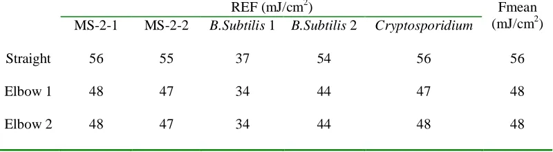
The UV fluence distributions were used to compute the log inactivation and

reduction equivalent fluence (REF) for microorganisms used in Bohrerova et al. (2006)

(two MS-2 and two Bacillus Subtilis spores) and Cryptosporidium from Qian et al. (2004).

Two Cabaj models (Cabaj and Sommer, 2000) were applied to replicate UV

fluence-response kinetics for the two surface batches of the Bacillus Subtilis spores experimental

kinetics data used in Bohrerova et al. (2006). A first order model was used to capture the

kinetics of the MS-2 data from Bohrerova et al. and Cryptosporidium from Qian et al.. A

least squares fit was used to optimize the model constants. The kinetics are displayed in

Figure 11. Table 2 displays the computed REF results. The two kinds of MS-2 and

Cryptosporidium experimental data followed the log-linear UV fluence-response kinetics

while Bacillus Subtilis spores followed a log-non-linear UV fluence-response kinetics

based on the Cabaj-Sommer model, which includes a shoulder in the low UV fluence

region and a tail in the high UV fluence region quite well. As can be seen in Table 2, both

MS-2 kinetics, Cryptosporidium kinetics, and B. Subtilis 2 kinetics predicted similar REF

values for the three configurations as with the average UV fluence value computed by the

Bayesian model. However, B. Subtilis 1 was not as sensitive as the other biological

indicators in detecting the difference in performance between the elbow configurations

and the straight pipe configuration and predicted a lower overall REF for all three

(22)

kinetics was log-linear in the UV fluence region (20 to 40 mJ/cm2) where the greatest

change in the UV fluence distributions between the elbows and straight configuration

occurred. Therefore, the log-non-linear UV fluence-response kinetics did not impact the

sensitivity of B. Subtilis 2 in detecting the impact of the design change on the UV reactor

performance.

These results seem to support some of the experimental biodosimetry data in the

literature that displayed a decrease in the REF with the presence of an upstream elbow

compared to the straight pipe configuration for a pilot-scale single lamp LP UV reactor

(Ducoste et al., 2005). Ducoste et al. also reported CFD modeling results for their single

lamp reactor and showed that the predicted UV fluence distribution for the straight pipe

configuration also shifted to a higher UV fluence fluence range compared to the elbow

configuration UV fluence distribution. However, the results displayed in Figure 10 did not

reveal an elbow configuration that was better than the straight pipe configuration as

predicted by Ducoste et al. (2005) for a full-scale multilamp medium pressure (MP) UV

reactor. Ducoste et al. (2005) theorized that a perpendicular elbow configuration similar

to Figure 2C would produce a rotating flow that may enhance the log reduction through

longer path lengths in the reactor. However, the results in Figure 10 suggest that whether

a rotating flow enhances the log reduction may be a strong function of the reactor design.

A single LPHO lamp located at the center of the reactor diameter may not be as sensitive

to a rotating flow compared with a reactor that contains four MP lamps located off center.

In addition, the UV reactor lamp in this study has an arc length that is not long enough to

(23)

longer arc length UV lamp was not selected in this reactor design to reduce any chance of

significant reactor wall degradation since the reactor is made of PVC pipe. Consequently,

a small dark zone exists in the influent region.

These subtle changes in reactor design can influence how the reactor behaves

under the influence of different upstream hydraulic configurations. The results in Figure

10 may further suggest that the possible occurrence of an upstream elbow configuration

that performs better than an upstream straight pipe configuration may be very limited.

Although the UV fluence results for elbow 1 and elbow 2 look the same, it is possible that

either the Bayesian model or the fluorescent microspheres may not be sensitive enough to

capture subtle difference between the two elbow hydraulic conditions. In order to test the

sensitivity of the Bayesian model, an ideal normal fluorescence distribution had been

developed to mimic the reactor microspheres’ fluorescence distribution.

Bayesian Model Sensitivity

In this sensitivity analysis, a UV fluence distribution had been computed using the

Bayesian model by 1) keeping a constant average of the ideal normal fluorescence

distribution and changing the standard deviation and 2) changing the average value but

keeping a constant standard deviation. A mid level UV fluence region (around 50 mJ/cm2)

and a low level UV fluence region (around 20 mJ/cm2) had been explored in Table 3.

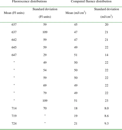
Based on the results in Table 3, the Bayesian model does not seem to display a

strong sensitivity in detecting a change in the standard deviation of the microspheres’

(24)

fluorescence units (Fl), there was only a corresponding change in the mean of UV fluence

of ±1 mJ/cm2 and 1 mJ/cm2 change in the standard deviation. The only exception is when

the microspheres’ fluorescence standard deviation went down to 29 (Fl), the UV fluence

distribution displayed a significant change in standard deviation (8 mJ/cm2) and

distribution shape although the UV fluence average still remained within 1 mJ/cm2 of the

other values.

In contrast with standard deviation sensitivity, the Bayesian model was quite

sensitive to changes in the average of the microspheres’ fluorescence distribution. A

change in the average of 10 fluorescence units (637 to 647 Fl) produced a corresponding

change in the average of 5 mJ/cm2. However, this corresponding change between

fluorescent units and UV fluence seems to decrease in the low fluence range since a

change in the average of 10 fluorescence units (714 to 724 Fl) produced a change in the

average UV fluence of 3 mJ/cm2. Consequently, the sensitivity of fluorescence

microspheres for detecting subtle changes in the design configuration or operating

condition in the low fluence region may be limited due to the overlapping nature of the

microspheres’ fluorescence data with known UV fluences in the collimated beam

experiments.

The experimental continuous-flow microspheres’ fluorescence distribution

statistics are compared in Table 4 for the three configurations. The results in Table 4

display similar agreement with the Bayesian model sensitivity conclusion. Compared

with the two elbow configuration tests, the straight pipe inlet configuration test had

(25)

using the Bayesian model. However, the two elbow configuration tests had the same

average fluorescence value and similar standard deviation. In this case, the results for the

experimental microspheres indicate identical performance between the two elbow

conditions.

Relationship with Biodosimetry

The performance of a UV reactor is currently validated using biodosimetry, which

measures the log inactivation of a non-pathogenic surrogate through a UV reactor and

back-calculates the reduction equivalent fluence (REF) from a known UV

fluence-response curve (Qualls and Johnson 1983). The non-pathogenic surrogates that have been

commonly used for validating UV reactor treatment efficiency are MS-2 coliphage and

Bacillus subtilis spores. However, there are some challenges of computing the REF

predicted by biodosimetry. These challenges include the following:

1. REF predicted by MS-2 and Bacillus subtilis is not consistent (a maximum of 30%

difference) for the same UV reactor under certain conditions (Bohrerova et al. 2006).

2. It has been shown that only microbial surrogates with similar sensitivity to the target

pathogen can detect the reactor hydraulic inefficiencies from the REF value (Mackey

et al. 2002).

3. Bacillus subtilis does not have the same sensitivity in the whole range of UV fluence

due to its complex UV inactivation kinetics. The kinetics of UV inactivation of

Bacillus subtilis contain a shoulder in the limit of low fluences, followed by

roughly first-order inactivation, then followed by tailing (Nicholson and Galeano

(26)

The results in Table 2 did show that the REF predicted using Bacillus subtilis 1

could significantly deviate from other biological surrogates. However, this deviation was

a strong function of the kinetics since another batch of Bacillus subtilis (2) had similar

REF results compared to other biological surrogates in Table 2. Furthermore, the results

in Table 2 seem to contradict in part the concept that the UV response kinetics of the

biological surrogate had to be similar to the target pathogen. In Table 2, Cryptosporidium

UV response was 3.8 times greater than MS-2-1 and 4.4 times greater than MS-2-2. Yet,

the MS-2 REF values were similar to Cryptosporidium REF value for both the elbow

configurations and the straight pipe configuration. Based on the predicted REF similarity

between MS-2 and Cryptosporidium, the requirement should be that the biological

surrogate should have the same shape in the UV response kinetics over the fluence region

being tested.

The challenges described with the biodosimetry method make the current UV

reactor validation not comprehensive and inconsistent. In order to improve the UV reactor

validation process, fluorescent microspheres using the Bayesian approach could be used

as an additional test since a) it provides consistent results for the same reactor

configuration; and b) the fluorescent microspheres kinetics due to exposure to UV

irradiation follows a linear relationship, which provides the same UV sensitivity in the

(27)

Conclusions

A study has been performed to evaluate the UV reactor fluence distribution under

multiple upstream configurations using UV sensitive fluorescent microspheres.

Experimental tests were performed at 51 gpm flow rate, 91% UV transmittance (UVT) on

a single lamp low-pressure high-output (LPHO) UV reactor with two kinds of 90- degree

bends and one straight pipe configuration. The results illustrated that the fluorescent

microspheres using the Bayesian approach was able to characterize the change in UV

reactor performance due to changes to upstream hydraulic configurations. The result for

the straight pipe inlet configuration demonstrated a higher UV fluence mean value and

the distribution curve shifted to a higher UV fluence region. Compared to the fluence

distributions from both elbow configurations, the UV fluence distribution curves of the

two elbow configurations overlapped each other and produced the same mean value and

standard deviation. The results also showed that the Bayesian approach was quite

sensitive to changes in the average of the microspheres’ fluorescence distribution

although it did not display a strong sensitivity in detecting a change in the standard

deviation for the microspheres’ fluorescence distribution. Overall, the fluorescent

microspheres Bayesian approach can serve as an additional test to biodosimetry for UV

reactor validation by providing unbiased UV fluence distribution assessment of design

(28)

References

Anderson, W. A., Zhang, L., Andrews, S. A., Bolton, J. R. (2003) “A technique for direct measurement of UV fluence distribution.” In Proceedings of the Water Quality Technology Conference; American Water Works Association: Philadelphia, PA, 2003.

Baeza, C., Ducoste, J. J. (2004) “A non-biological surrogate for sequential disinfection processes.” Water Res., 38, 3400-3410.

Blatchley, E., Shen, C., Naunovic, Z., Lin, L., et al. (2006) “Dyed Microspheres for Quantification of UV Dose Distributions: Photochemical Reactor Characterization by Lagrangian Actinometry.” J. Environ. Eng., 132(11), 1390-1403.

Bohrerova, Z., Bohrer, G., Mohan Mohanraj, S., Ducoste, J. J., and Linden, K. G.. (2005) “Experimental measurements of fluence distribution in a UV reactor using fluorescent microspheres.” Environ. Sci. Technol., 39(22), 8925–8930.

Bohrerova Z., Mamane H., Ducoste J.J., and Linden, K. G.. (2006) “Comparative inactivation of Bacillus subtilis spores and MS-2 coliphage in a UV reactor: Implications for validation” J.Environ. Eng-ASCE 132 (12), 1554-1561

Bolton, J. R., and Linden, K. G. (2003). “Standardization of methods for fluence (UV dose) determination in bench-scale UV experiments.” J.Environ. Eng., 129(3), 209–215.

Cabaj, A., Sommer, R., (2000) “Measurement of Ultraviolet Radiation with Biological Dosimeters”, Radiation Protection Dosimetry, 91, 139-142.

Dai, X. J., Hozalski, R. M. (2003) “Evaluation of microspheres as surrogates for Cryptosporidium parvum oocysts in filtration experiments.” Environ. Sci. Technol. 37, 1037-1042.

Ducoste, J.J., Liu, D., Linden, K.G., Zuzana, H., Mamane-Gravetz, (2005) “Impact of Influent Pipe Configuration on UV Reactor Performance: Is the Elbow Truly the Worst Case Hydraulic Condition.” Proceedings WEF Disinfection Conference, Phoenix, AZ, February 6-9

Ducoste, J.J. and Linden, K.G., (2006) “Hydrodynamic Characterization of UV Reactors.” American Water Works Association Research Foundation, Denver, CO.

(29)

Mackey, E. D., Hargy, T. M., Wright, H. B., Malley, J. P., and Cushing, R. S. (2002) “Comparing Cryptosporidium and MS2 bioassays— Implications for UV reactor validation.” J. Am. Water Works Assoc., 94 (2), 62–69.

Marinas, B. J., Rennecker, S., Teefy, S., Rice, E. W. (1999) “Assesing ozone disinfection with nonbiological surrogates.” J. Am, Water Works Assoc. 91, 79-89.

Nicholson, W. L., and Galeano, B. (2003). “UV resistance of Bacillus anthracis spores revisited: Validation of Bacillus subtilis spores as UV surrogates for spores of B-anthracis Sterne.” Appl. Environ. Microbiol., 69(2), 1327–1330.

Qian, SS., Donnelly, M., Schmelling, DC. (2004). “Ultraviolet light inactivation of protozoa in drinking water: a Bayesian meta-analysis.” Water Research, 38(2), 317-326

Qualls, R.G., and Johnson, J.D. (1983). “Bioassay and dose measurement in UV disinfection.” Appl. Environ. Microbiol., 45(3), 872–877.

Rahn, R. (1997) “Potassium Iodide as a Chemical Actinometer for 254 nm Radiation: Use of Iodate as an Electron Scavenger” Photochemistry and Photobiology. 66(4), 450-455.

USEPA (2006) EPA 815-R-06-007 “Ultraviolet Disinfection Guidance Manual for the Final Long Term 2 Enhanced Surface Water Treatment Rule.” November 2006, USEPA, Office of Water (4601)

Wright, H., Mackey, E., (2003) “Strategies for Validating Large-scale UV Reactors.” In

(30)

Table 1: Flow conditions and analyses of effluent water spiked with microspheres for continuous-flows tests.

Flow (gal./min) 51

Water transmittance (%) 91.1

UV Absorbance (254nm) 0.0403

pH 7.77

Free chlorine 0.02 (Raw water 2.14) Quenched chlorine concentration (mg/L)

(31)

Table 2: Reduction equivalent fluence (REF) computed for MS-2, Bacillus Subtilis and

Cryptosporidium with fluence distributions results for three configurations. The average UV fluence predicted by the Bayesian model (Fmean) was also compared.

REF (mJ/cm2)

MS-2-1 MS-2-2 B.Subtilis 1 B.Subtilis 2 Cryptosporidium

Fmean

(mJ/cm2)

Straight 56 55 37 54 56 56

Elbow 1 48 47 34 44 47 48

(32)

Table 3: UV fluence distribution mean and standard deviation computed using Bayesian model.

Fluorescence distributions Computed fluence distribution

Mean (Fl units)

Standard deviation

(Fl units)

Mean (mJ/cm2)

Standard deviation

(mJ/cm2)

637 59 45 20

637 109 47 21

642 59 47 21

645 59 49 22

647 29 51 14

" 49 50 22

" 54 50 22

" 59 50 22

" 69 49 22

" 79 49 22

" 109 51 23

714 70 18 8.0

719 " 19 8.6

(33)

Table 4: Mean and standard deviation of the experimental continuous-flow microspheres’ fluorescence distribution for the three upstream configurations.

Straight Elbow 1 Elbow 2

Microspheres’ fluorescence

mean (Fl)

649

(95% CI: 646-651)

672

(95% CI: 665-675)

672

(95% CI: 665-675)

Microspheres’ fluorescence

standard deviation (Fl)

(34)

Figure 1: Photograph of LPHO UV reactor

Reactor

inlet

(35)

Figure 2: AutoCAD designs of three inlet configurations. A: Straight pipe configuration; B: 90 elbow horizontal configuration (Elbow 2); C: 90 elbow vertical configuration (Elbow 1).

A B C

(36)

Figure 3: Photograph of pilot test configurations.

Water from pump

turbine flow meter

(37)

Figure 4: Photograph of pilot test that display injection and sampling points.

Microspheres spiking point

(38)

(39)

(40)

0 10 20 30 40 50 60 70 80 90

200 300 400 500 600 700 800 900 1000

Fluorescence Internsity

C

o

u

n

ts

0 mJ/cm2

40 mJ/cm2

120 mJ/cm2

(41)

Fl mean= -1.76UV fluence + 652.04 R2 = 0.9577

Fl std = -0.16UV fluence + 80.32 R2 = 0.9698

0 100 200 300 400 500 600 700 800

0 20 40 60 80 100 120

UV Fluence (mJ/cm2)

F

lu

o

re

s

c

e

n

c

e

i

n

te

n

s

it

y

(42)

0 10 20 30 40 50 60

200 300 400 500 600 700 800 900 1000

Fluorescence intensity

C

o

u

n

ts

Control (without UV)

51gpm, straight inlet configuration

(43)

0 0.005 0.01 0.015 0.02 0.025 0.03 0.035 0.04 0.045 0.05

0 20 40 60 80 100 120 140 160 180 200

Fluence (mJ/cm2)

f(

F

lu

e

n

c

e

)

Straight: Avg=56mJ/cm2, Sd=25mJ/cm2

Elbow 1: Avg=48mJ/cm2, Sd=21mJ/cm2

Elbow 2: Avg=48mJ/cm2, Sd=21mJ/cm2

(44)

0 0.5 1 1.5 2 2.5 3 3.5 4 4.5 5

0 10 20 30 40 50 60

UV Fluence (mJ/cm2)

L o g I n a c ti v a ti o n ( N o /N ) MS-2-1 MS-2-2 Cryptosporidium B.Subtilis-1 B.Subtilis-2

(45)

(46)

Appendix A: Statistical analysis procedures

1. Extract microspheres fluorescent data using Summit v4.3

(1) Input flow cytometry raw data into Summit v4.3.

(2) Change histogram scale to 1024 for fluorescence value.

(3) Save data as txt file.

2. Use Matlab program to transform txt file into csv files.

Matlab program:

cd 'C:\xi\Research\UV\test\06-28\matlab\txt'

a(:,1) = textread('062807B #0 Sample_2 _405 NM Lin.txt');

xlswrite ('CB.xls',a);

3. Prepare csv input files for R 2.5.0 alpha

(1)Upload R2WinBUGS package to R 2.5.0 alpha at the start of using R 2.5.0 alpha.

(2)First csv file: collimated-beam fluorescence data transferred from matlab under

different UV fluence levels (DataCBWinBUGS.csv).

(3)Second csv file: continuous-flows reactor test fluorescence data transferred from

matlab (DataReactorWinBUGS.csv).

(4)Manually gate noise which was caused from flow cytometer: change noise value

(47)

(5)Third csv file (DataParamsWinBUGS.csv): parameters related to statistical

calculation:

• NCB: number of observations in each collimated beam dose level

• UVCB: UV dose in collimated beam that correspondent to NCB

• Gatemin: lowest gated brightness observation

• gatemax: highest gated brightness observation

• Nreactor: number of observations in reactor

• Ntot: total number of observations including collimated beam and reactor

• NCat: number of UV dose levels in collimated beam

4. Calculate best estimate for B μ, A μ, B σ, A σ, and regenerate observations for reactor,

and prepare initiate value for MCMC chains with R 2.5.0 alpha.

R program:

CBDat<-read.csv("C:\\xi\\Research\\UV\\test\\06-28\\bugs\\straight pipe\\normal\\DataCBWinBUGS.csv", header =

TRUE, sep = ",", quote="\"", dec=".",fill=TRUE)

ReactorDat<-read.csv("C:\\xi\\Research\\UV\\test\\06-28\\bugs\\straight pipe\\normal\\DataReactorWinBUGS.csv",

header = TRUE, sep = ",", quote="\"", dec=".",fill=TRUE)

ParamDat<-read.csv("C:\\xi\\Research\\UV\\test\\06-28\\bugs\\straight pipe\\normal\\DataParamsWinBUGS.csv",

header = TRUE, sep = ",", quote="\"", dec=".",fill=TRUE)

NCB <- ParamDat[,1] #num observations in CB

UVCB <- ParamDat[,2] # UV dose in CB

gatemin <- ParamDat[1,3] #lowest gated brightness observation

gatemax <- ParamDat[2,3] #highest gated brightness observation

Nreactor <- ParamDat[1,4]#num observations in reactor

NFl <- ParamDat[1,5] #total # observations

NCat <- ParamDat[1,6] #number of UV dose levels in CB

FlCatInd <- vector('numeric',(NCat+1))*0

(48)

avgCB <- vector('numeric',(NCat))*0

UVreactor <- vector('numeric',Nreactor)*0

maxdose <- 400 #highest possible UV dose in reactor

mindose <- 0

skw <- 5 #minimal skew parameter for Gamma

#calculate cumulative index start points

for (cat in 2:(NCat+1)) {

FlCatInd[cat] <- sum(NCB[1:(cat-1)])

} #end cat

Fl <- vector('numeric',FlCatInd[NCat+1])*0

FlR <- vector('numeric',Nreactor)*0

#regenerate observations for CB

ind <- 0

for (cb in 1:NCat) {

for (i in gatemin:gatemax) {

if (CBDat[i,cb] > 0 ) {

Fl[(ind+1):(ind+CBDat[i,cb])] <- i

ind <- ind+CBDat[i,cb]

} #end if

} #end i

stdCB[cb] <- sd(Fl[(FlCatInd[cb]+1):(FlCatInd[cb]+NCB[cb])])

avgCB[cb] <-

mean(Fl[(FlCatInd[cb]+1):(FlCatInd[cb]+NCB[cb])])

} #end cb

glmSTD <- glm(stdCB ~ UVCB, family=gaussian)

OmegaSD <- solve(vcov(glmSTD))

meanSD <- coefficients(glmSTD)

glmAVG <- glm(avgCB ~ UVCB, family=gaussian)

OmegaA <- solve(vcov(glmAVG))

meanA <- coefficients(glmAVG)

#regenerate observations for reactor

indR <- 0

for (i in gatemin:gatemax) {

if (ReactorDat[i,1] > 0 ) {

FlR[(indR+1):(indR+ReactorDat[i,1])] <- i

(49)

} #end if

} #end i

MeanReactor <- (mean(FlR)-meanA[1])/meanA[2]

mu1 <- meanA[1]

mu2 <- meanA[2]

tau1 <- meanSD[1]

tau2 <- meanSD[2]

bugs.data(c("FlR","mu1","mu2","tau1","tau2","Nreactor","skw"),

dir=("C:\\xi\\Research\\UV\\test\\06-28\\bugs\\straight

pipe\\normal\\min"),digits = 5)

UVreactor <- vector('numeric',Nreactor)+MeanReactor

gr<- skw+0.1

gmu<-0.05

bugs.data(c("UVreactor","gr","gmu"),dir=("C:\\xi\\Research\\UV

\\test\\06-28\\bugs\\straight

pipe\\normal\\min\\init1\\"),digits = 5)

UVreactor <- vector('numeric',Nreactor)+MeanReactor+10

gr<- skw+0.8

gmu<-0.001

bugs.data(c("UVreactor","gr","gmu"),dir=("C:\\xi\\Research\\UV

\\test\\06-28\\bugs\\straight

pipe\\normal\\min\\init2\\"),digits = 5)

bugs.data(c("Fl"),dir=("C:\\xi\\Research\\UV\\test\\06-28\\bugs\\straight pipe\\normal\\min\\Fl\\"),digits = 5)

5. Use WinBUGS 1.4 to iterate over the probable range of the B μ, A μ, B σ, A σ parameter

values and converges to the most probable set of values.

(1) WinBUGS model:

model {

for (i in 1:Nreactor) {

FlR[i] ~ dlnorm(mu[i],tau[i])

mu[i] <- log(mu1+mu2*UVreactor[i])

tau[i] <- tau1+tau2*UVreactor[i]

UVreactor[i] ~ dgamma(gr, gmu)

(50)

gr ~ dpar(1, skw)

gmu ~ dexp(0.001)

}

(2) Procedures:

• In WinBUGS, load model then click (1) model (2) specification (3) check

model. A message saying "model is syntactically correct" should appear in the

bottom left of the WinBUGS program window.

• Open data file generated by R, then click once with the load data button in the

Specification Tool window. A message saying "data loaded" should appear in

the bottom left of the WinBUGS program window.

• Type the number 2 in the white box labeled number of chains in the

Specification Tool window. In the current approach, only two chains were

necessary. Next compile the model by clicking once on the compile button in

the Specification Tool window. A message saying "model compiled" should

appear in the bottom left of the WinBUGS program window.

• Open “initial value 1” data file generated by R, click once on the load inits

button in the Specification Tool window. A message saying "initial values

loaded: model contains uninitialized nodes " should appear in the bottom left

of the WinBUGS program window. Next open “initial value 2” data file

generated by R and repeat this process for the second initial values file. A

message saying "initial values loaded: model initialized" should now appear in

the bottom left of the WinBUGS program window.

(51)

box marked node; Click set button once; Repeat for gmu. Type * in the white

box then click trace button once to trace both gr and gmu while model running.

• Update model: Select the Update... option from the Model menu. Click once

on the update button: the program will now start simulating values for each

parameter in the model.

6. Prepare shape (gmu) and rate (gr) parameters generated by WinBUGS: After

WinBUGS finished updating, select Samples... from the Inference menu; type “gmu”,

“gr” under separate instances in the white box marked node; click once coda for each

and copy 1000 “gmu” and “gr” values for each chain into a csv file.

7. Use R 2.5.0 alpha to resample from each Gamma distribution and regenerate the UV

fluence distribution in the reactor.

R program:

Dat<-read.csv("C:\\xi\\Research\\UV\\test\\06-28\\bugs\\straight pipe\\normal\\output.csv", header = TRUE,

sep = ",", quote="\"", dec=".",fill=TRUE)

converge <- 50

Ndat <- length(Dat[,1])

N <- Ndat-converge+1

#shape=mu, rate = r

Shape <- vector('numeric',2*N)*0

Rate <- vector('numeric',2*N)*0

Numloop <- 100

result <- vector('numeric',2*Numloop*N)*0

Rate[1:N] <- Dat[converge:Ndat,2]

Rate[(N+1):(2*N)] <- Dat[converge:Ndat,3]

Shape[1:N] <- Dat[converge:Ndat,4]

Shape[(N+1):(2*N)] <- Dat[converge:Ndat,5]

(52)

for (i in 1:(2*N)) {

result[(j-1)*(2*N)+i] <-

rgamma(1,shape=Shape[i],rate=Rate[i])

}

brek <- c(0:1000)*(max(result))/1000

HIST <- hist(result,breaks=brek)

UV_Dose <- HIST$mids[1:1000]

Probability <- HIST$density[1:1000]

write.csv(UV_Dose,file="C:\\xi\\Research\\UV\\test\\06-28\\bugs\\straight pipe\\normal\\min\\R\\data1.csv")

(53)

Appendix B: Experimental protocol for collimated beam calibration and radiometer

validation

1. Average fluence (UV dose) determination by radiometer

Correction factors

A. Reflection Factor:

Reflection factor accounts for the reflection when the beam comes from one media to

another. For air and water, reflection factor is 0.975, and represents the fraction of the

incident beam that enters the water.

B. Petri Factor

Petri factor is defined as the ratio of the incident irradiance average over the Petri dish

area to the irradiance at the center of the dish and is used to correct the irradiance reading

at the center of the Petri dish to more accurately reflect the average incident fluence rate

over the surface area.

Steps:

a) Vertically scan the radiometer detector over the Petri dish area every 2 grids

(2.39mm/grid) on the marked graph paper.

b) Horizontally scan the radiometer detector over the Petri dish area every 2

grids (2.39mm/grid) on the marked graph paper.

c) Divide the irradiance at each point by the center irradiance to be the ratio

value.

d) Multiply the vertical ratio value by the horizontal ratio to get the point total

(54)

e) Take the average of the entire total ratio to be the Petri Factor.

In general, a well designed collimated beam apparatus should deliver a Petri Factor

greater than 0.9.

C. Water Factor

Water factor accounts for the decrease in irradiance arising from absorption as the beam

passes through the water.

) 10 ln( 10 1 Factor Water l l a a − − =

a: absorbance for a 1cm path length at 254nm.

ℓ:vertical path length (cm) of the water in the Petri dish.

D. Divergence Factor

l

+

=

L

Factor

Divergence

L: distance from the UV lamp to the surface of the cell suspension (cm).

ℓ:vertical path length (cm) of the water in the Petri dish.

Average Fluence calculation:

Fuenceavg = E0 × Petri Factor × Reflection Factor × Water Factor × Divergence Factor × t

E0: radiometer reading at the center of the Petri dish area.

t: exposure time

2. Fluence determination by iodide/iodate actinometry

Solutions preparation

(55)

Na2B4O7•10H2O and 21.4 g of KIO3 to 1 L of distilled water.

Solution B: On the day of an experiment, add sufficient iodide to make the

concentration of iodide 0.60 M. For example, add 24.9 g of KI to 250 mL of Solution

A and stir until dissolved.

Actinometry Procedure

a). Add 10 mL of Solution B to a 50 × 35 mm petri dish. Place in position and center under the UV light in the bench scale apparatus and leave for 1 min while UV

light off. Using deionized water as baseline to zero the spectrophotometer.

Determine the absorbance at 352 nm as blank run.

b). Add 10 mL of Solution B to the 50 × 35 mm petri dish and center under the UV light. Do this three times with targeted irradiation times (for example, 30, 45 and

60 s). After irradiation each solution, determine the absorbance at 352nm.

Fluence calculations E A l V A A cs o × Φ − = 352 352 352 ) ( Fluence

ε (mJ cm-2)

A₃₅₂o =absorbance at 352 nm for blank run (unitless)

A352 = absorbance at wavelength 352nm at time t (unitless)

l = pathlength of the spectrophotometer cuvette (cm)

ε352 = molar absorption coefficient of actinometer at 352nm (26400 M-1.cm-1)

Φ = quantum yield at the irradiating wavelength (e.g. 0.64 × [1 + 0.02 ×

(56)

Temp = actinometer temperature during irradiation (°C)

V = volume of irradiated actinometer solution (0.01 L)

Acs = cross sectional area (17.20 cm2)