1
P a g e
Robust Product Design: A Modern View of Quality Engineering in
Manufacturing Systems
Amir Parnianifarda1, A.S. Azfanizama, M.K.A. Ariffina, M.I.S. Ismaila
a.Department of Mechanical and Manufacturing Engineering, Faculty of Engineering, Universiti Putra Malaysia, 43400 UPM Serdang, Selangor, Malaysia.
ABSTRACT:
One of the main technological and economic challenges for an engineer is designing high-quality products in manufacturing processes. Most of these processes involve a large number of variables included the setting of controllable (design) and uncontrollable (noise) variables. Robust Design (RD) method uses a collection of mathematical and statistical tools to study a large number of variables in the process with a minimum value of computational cost. Robust design method tries to make high-quality products according to customers’ viewpoints with an acceptable profit margin. This paper aims to
provide a brief up-to-date review of the latest development of RD method particularly applied in manufacturing systems. The basic concepts of the quality loss function, orthogonal array, and crossed array design are explained. According to robust design approach, two classifications are presented, first for different types of factors, and second for different types of data. This classification plays an important role in determining the number of necessity replications for experiments and choose the best method for analyzing data. In addition, the combination of RD method with some other optimization methods applied in designing and optimizing of processes are discussed.
KEYWORDS: Robust Design, Taguchi Method, Product Design, Manufacturing
Systems, Quality Engineering, Quality Loss Function.
1.
Corresponding Author: Amir Parnianifard
Tel: 00989138207031 Email: parniani@hotmail.com Orcid Id: 0000-0002-0760-2149
2
P a g e
1. Introduction
In a new comprehensive world with varieties of industrials, rapid progress in technology cause that all company and organization in all type of industries have to improve and adjust their processes according to latest changes. Moreover, in each company, flexibility is an essential matter for preserving their productivity, efficiency and keeping their survival among other rivals. So, companies must remain in the best condition (flexible) among rapid progress in technology and change in product’s specification. Therefore, most techniques and methods have been presented to help engineers for designing the company's processes to achieve the highest quality with at least costs. Nowadays, one of the main techniques that have been applied to achieve aforesaid purpose is quality engineering. Quality engineering is an interdisciplinary science which is concerned with not only producing satisfactory products for customers but also reducing the total loss (manufacturing cost plus quality loss). The Robust Design (RD) is one of the main tools that have been used in quality engineering [1].
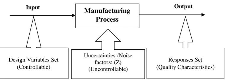
The most processes are affected by external uncontrollable factors in real condition, which cause that quality characteristics are far from ideal points and have variation. Figure 1 illustrates an overview of manufacturing processes with input (also called design factors), output (also called response factors), and noise factors (also called environmental factors).
Approximate location of Figure 1
In process robustness studies, it is desirable to minimize the influence of noise factors and uncertainty on the process and simultaneously determine the levels of input and control factors which optimizing the overall responses, or in another sense, optimizing product and process which are minimally sensitive to the various causes of variance. [2] has defined some traits for the RD method in manufacturing systems, consist of:
• Making product performance robust against raw material variation. So, it allows
using the wide grade of materials and their components.
• Making product designs insensitive to manufacturing variation in order to reduce
3
P a g e
• Designing the product least sensitive to the variation in the operating environment in order to enhance reliability and decrease operating cost.
• Using a new structure of process development, thus engineering time is used most
productively.
This paper aims to provide up-to-date review through latest development on robust product design and its application in manufacturing systems. This paper tries to discuss how the RD works in designing products while its contribution to the quality subject is highlighted. The outcomes are focused to imply the advantages of this method on the ideal function of manufacturing processes.
The rest of this paper is organized as follows. Section 2 provides basic information on robust design methodology. In section 3 the application of robust design in different manufacturing systems are reviewed among studies in literature when combined with two types of model-based and metamodel-based optimization approaches. Section 4 presents the brief discussion over strength and weakness points of RD. This paper is concluded in section 5.
2. Basic of Robust Design (RD)
4
P a g e
environmental changeability and component variations. Totally, a designing process that has a minimum sensitivity to variations in uncontrollable factors is the end result of robust design. The foundation of robust design has been structured by Taguchi on parameter design in a narrow sense. The concept of robust design has many aspects, which three aspects among them are more outstanding [1]:
1- Investigating a set of conditions for design variables which are insensitive (robust) against noise factor variation
2- Finding at least variation in a performance around target point
3- Achieving the minimum number of experiments by employing orthogonal arrays
Robust design based on Taguchi approach has employed some statistically and analytically tools such as orthogonal arrays and Signal to Noise (SN) ratios. Furthermore, many designed experiments for determining the adequate combination of factor levels which are used in each run of experiments and for analyzing data with their interaction have been applied a fractional factorial matrix that called Orthogonal Arrays (OA). The ratio between the power of the signal and the power of noise is called the signal to noise ratio (𝑆𝑁 = 𝑝𝑜𝑤𝑒𝑟 𝑜𝑓 𝑠𝑖𝑔𝑛𝑎𝑙 𝑝𝑜𝑤𝑒𝑟 𝑜𝑓 𝑛𝑜𝑖𝑠𝑒⁄ ). The larger numerical value of SN ratio is more desirable for process. There are three types of SN ratios which available in robust design method depending on the type of quality characteristic, Larger The Better (LTB), Smaller the Better (STB), Nominal The Best (NTB). Both concepts of signal to noise ratio and orthogonal arrays have been described by most studies after first introducing by Taguchi in 1980s, so for more information see [1], [2], [4].
2.1 Quality Loss Function (QLF):
5
P a g e
factors and uncertainty in the process and simultaneously determines the levels of input and control factors, which optimizing the overall responses, or in another sense, optimizing product and process, which is minimally sensitive to the various causes of variance. By employing the information of experiments about the relationships between input control factors and output responses, robust design methods can disclose robust solutions that are less sensitive to causes of variations [5]. It is commonly accepted that the Taguchi’s principles are useful and very appropriate for industrial product design [6].
Dr. Taguchi represented the concept of quality loss as an average amount of total loss that compels to society because of deviating from the ideal point and variability in responses. Moreover, this function tries to make a trade-off between the mean and variance of each type of quality characteristics [1]. Figure 2 depicts the graphical concepts of expected QLF on the classification of quality characteristics into three different types of nominal the best (NTB), smaller the better (STB), and larger the better (LTB).
Approximate location of Figure 2
In addition, QLF based on Taguchi’s approach for all three types of quality characteristics are presented in below.
where 𝜇 , 𝜎2, 𝑇 respectively are quality characteristic mean, variance, and target and 𝐶 0
is loss coefficient. The value of 𝐶0 is computed by 𝐴0
∆2 for NTB and STB and 𝐴0∆ 2 for
LTB. The quality loss coefficient 𝐶0 can be determined on the basis of information about the losses in monetary terms caused by falling outside the customer tolerance. The coefficient 𝐶0plays an important role to make the expected loss function in monetary loss scales. In addition, 𝐴0 is introduced as a cost of repair or replacement when the quality characteristic performance has the distance of ∆ from target point [2].
NTB 𝐿(𝑦) = 𝐶0[(𝜇 − 𝑇)2+ 𝜎2] (1)
STB 𝐿(𝑦) = 𝐶0[𝜇2+ 𝜎2] (2)
LTB 𝐿(𝑦) = 𝐶
0[( 1
𝜇2)(1 + 3𝜎
6
P a g e
[7] have proposed the same formula for all three types of quality characteristics with more simplicity in the relevant formulation. Their proposed formula is based on lack of accessing target to infinity for LTB case, in order to it is unachievable. All three types of expected quality loss, which aforementioned could be replace by the proposed formulation as below:
where 𝛼 is equal to 𝑇
𝜇 when 0 ≤ 𝛼 ≤ 𝑚 and 𝑚 is a large number. The amount of 𝛼
could be defined by decision maker and 𝑇 is a target point for quality the characteristic. For different values of 𝛼 the expected loss represents different expected losses for each type of NTB, LTB, or STB. This value shows the shifting of 𝜇 to right or left side of target point and can be chosen zero for STB type, a large number more than one for LTB type and also 1 for NTB. But, it is strongly recommended that the target point and specially 𝛼 it does not need to be a large number or infinity for LTB cases, but it just needs to be significantly greater than one. In [7] and [8] has recommended that in the case of LTB the magnitude of 𝛼 needs to significantly greater than one but not necessarily a large number or infinity, and they suggested 𝛼 = 2 is appropriate to be employed in practice. In [9], the application of Eq.(4) has been expanded in multi-objective engineering deign problems.
2.2 Orthogonal Array (OA)
The OA design has the strength to allocate points in each corner of design space [10]. The OA was adapted to balance discrete experimental factors in a continues space [11]. The orthogonal array is a matrix with 𝑛 rows and 𝑝 columns where 𝑛 is number of experiments (input combination) and 𝑝 is number of input factors. Each factor is divided into 𝑚 equal size ranges (grids), and sample points are allocated to these orthogonal grid spaces. In general, the orthogonal array shows with symbol of 𝐿𝑛(𝑚𝑝), and has the
following properties:
• For the input factor in any column, every level happen 𝑛⁄𝑚 times.
• For the two input factors in any two columns, every combination of two levels happen
𝑛 𝑚2
⁄ times.
7
P a g e
• For the two factors in any two columns, all 𝑛 input combinations are combined by
levels as belows:
{(1,1), (1,2), ⋯ (1, 𝑚), (2,1), (2,2), ⋯ , (2, 𝑚), ⋯ , (𝑚, 1), (𝑚, 2), ⋯ , (𝑚, 𝑚)}
• By replacing any two columns of an orthogonal array, the remaining arrays are still
orthogonal to each other.
• By removing one or some columns of an orthogonal array, the remaining arrays are
orthogonal to each other, and OA is able to employ a smaller number of factors.
More information about constructing and implementing OA as computer experiments design has been provided in [11], [12].
2.3 Crossed array design
Taguchi proposed a crossed design approach for arranging the experiments in a noisy environment, while the process is influenced by environmental (noise) factors (see Figure 3).
Approximate location of Figure 3
In this arrangement, combinations of design variables are designed as an inner array (input combination), and noise factors are designed separately in outer array. For each input combination in inner array, all noise combinations in the outer array are experimented, see [1], [2].
2.4 Types of factors and data in RD
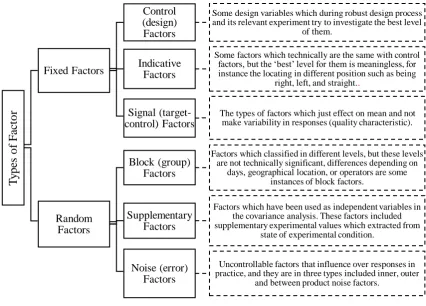
In robust design approach, two types of factors can treat in experiments, fixed and random types, as depicted in Figure 4 [13].
Approximate location of Figure 4
When the factor levels are technically controllable, it means these factors are ‘fixed’. In addition, levels in this types of factor can be reexamined and reproduced. ‘Random’
8
P a g e
experimental environment are usually divided into two different types of discrete and continuous. Taguchi has divided each of both types into three classes, as illustrated in Figure 5.
Approximate location of Figure 5
This classification plays an important role in deciding about a number of necessity replications for experiments and determines the best method for analyzing data [1], [4],
3. Hybrid RD with model-based and metamodel-based optimization methods
Robust design methodology has been advocated by most researchers in lots of different studies and it has been employed to improve the performance and quality of processes for various problems in the real world [14]. Since Genichi Taguchi has introduced his methods for off-line quality improvement in AT&T Bell laboratories in United State during 1980 till 1982, robust design method has been used in many areas in the real world of engineering [2]. The wide application of RD particularly based on Taguchi approach, have been attended to optimize the various manufacturing processes under noisy and uncertain condition. Taguchi RD is a functional approach that can be combined with other associated optimization methods particularly with two categories of robust engineering design approaches, included model-based and metamodel-based robust optimization techniques [15]. In model-based, the original model is not expensive in term of running experiments and model output can be used directly in optimization. [16] have presented a number of model-based robust optimization methods when used different scenarios set of uncertainty in the model. However, a model-based method on separate process components included the mean and the variance has been proposed by [18] which called dual response surface method.
9
P a g e
manufacturing industries. Metamodeling techniques have been developed from many different disciplines including statistics, mathematics, computer science, and various engineering disciplines [21]. Global search over design space is the main goal of model-based algorithms. Modern metamodels such as Kriging and Radial Basis Function (RBF) assisted optimization also derive global search. A metamodel or surrogate model by
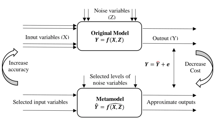
mathematical expression 𝑌̂ = 𝑓(𝑋, 𝑍)̂ can replace with true functional relationship 𝑌 = 𝑓(𝑋, 𝑍), where 𝑋 and 𝑍 denotes respectively design and noise (uncertain) factors. The
general overview of a metamodel with uncontrollable noise variables is illustrated in Figure 6.
Approximate location of Figure 6
There are different number of metamodels in literature such as different the order of polynomial regression, Kriging, RBF, and so on, for more information about metamodels techniques can refer to [6], [21]–[23]. Table 1 shows some main application of model-based and metamodel-model-based optimization methods which combined by RD approach in order to design and optimize manufacturing and production systems.
Approximate location of Table 1
Among searching articles, more concentration was undertaken on studies which have been implemented in recent years to warranty up-to-data reviewing results.
4. Strength and weakness viewpoints over RD
The vital role of noise × noise interaction in parameters design problems has been defended by [18]. In addition, the framework of these interactions defines the nature of non-homogeneity of process variance and typifies the design of parameters. The application of robust design optimization has been contributed by the great number of researchers in quality improvement of a various process or product design in practice, and several appropriate studies have been reviewed the application of Taguchi methodology in real case studies, see [15], [22], [24]–[27].
10
P a g e
approach in robust parameters design. The first one is the inefficiency of the signal to noise ratio. The second one is the shortage of ability in Taguchi design parameters to approach a flexible process modeling. The third one is the number of experiments in Taguchi robust design with their SN ratio that is not economical. Preoccupation with optimization is fourth, and fifth no formal allowance for sequential experimentation. The Taguchi approach with its crossed arrays and signal to noise ratios have emphasized the interaction between design variables with each other and have ignored the importance of interaction between design (control) and noise variables [18]. In addition, some other drawbacks have been connected to the traditional Taguchi’s approach. First, in designing variables with orthogonal arrays and signal to noise ratio, the process constraint is ignored for designing parameters, and second, robust design with Taguchi approach just deals with a single quality characteristic as a response in each run of the method. So, it could not propose the best design by considering all responses at the same time. Third, Taguchi method just investigates best levels of design variables in the discrete region and could not treat in whole design ranges [22], [27].
5. Conclusion:
In this paper, a brief overview of robust design method based on Taguchi worldwide viewpoint is provided. The main tools in RD included quality loss function, orthogonal array, and crossed array design are elaborated. In addition, the latest studies on RD method by combining some other optimization methods in two categories of model-based and metamodel-model-based are reviewed. At the end, the positive and negative viewpoints in academicals world over Taguchi robust design is sketched.
References:
1. S. Park and J. Antony, Robust design for quality engineering and six sigma. World Scientific Publishing Co Inc, 2008.
2. M. S. Phadke, Quality Engineering Using Robust Design. Prentice Hall PTR, 1989.
3. A. Shahin, Robust design: an advanced quality engineering methodology for change management in the third millennium, in Proceedings of the 7th International Conference of Quality Managers,
2006, pp. 201–212.
11
P a g e
5. V. T. Nha, S. Shin, and S. H. Jeong, Lexicographical dynamic goal programming approach to a robust design optimization within the pharmaceutical environment, European Journal of
Operational Research, 229, (2), pp. 505–517, 2013.
6. T. W. Simpson, J. D. Poplinski, P. N. Koch, and J. K. Allen, Metamodels for Computer-based Engineering Design: Survey and recommendations, Engineering With Computers, 17, (2), pp.
129–150, 2001.
7. N. K. Sharma, E. A. Cudney, K. M. Ragsdell, and K. Paryani, Quality Loss Function – A Common Methodology for Three Cases, Journal of Industrial and Systems Engineering, 1, (3), pp. 218–234,
2007.
8. N. K. Sharma and E. A. Cudney, Signal-to-Noise ratio and design complexity based on Unified Loss Function – LTB case with Finite Target, International Journal of Engineering, Science and
Technology, 3, (7), pp. 15–24, 2011.
9. A. Parnianifard, A. S. Azfanizam, M. K. A. Ariffin, and M. I. S. Ismail, Trade-off in robustness, cost and performance by a multi-objective robust production optimization method, International
Journal of Industrial Engineering Computations, 10, (1), pp. 133–148, 2019.
10. A. B. Owen, Orthogonal arrays for computer experiments, integration and visualization, Statistica Sinica, pp. 439–452, 1992.
11. J. R. Koehler and A. B. Owen, Computer experiments, in Handbook of statistics, 13, 1996, pp. 261–308.
12. Y. W. Leung and Y. Wang, An orthogonal genetic algorithm with quantization for global numerical optimization, IEEE Transactions on Evolutionary computation, 5, (1), pp. 41–53, 2001.
13. A. Parnianifard, A. S. Azfanizam, M. K. A. Ariffin, and M. I. S. Ismail, An overview on robust design hybrid metamodeling : Advanced methodology in process optimization under uncertainty, International Journal of Industrial Engineering Computations, 9, (1), pp. 1–32, 2018.
14. R. H. Myers, A. I. Khuri, and G. Vining, Response surface alternatives to the Taguchi robust parameter design approach, The American Statistician, 46, (2), pp. 131–139, 1992.
15. H. G. Beyer and B. Sendhoff, Robust optimization - A comprehensive survey, Computer Methods in Applied Mechanics and Engineering, 196, (33), pp. 3190–3218, 2007.
16. A. Ben-Tal, L. El Ghaoui, and A. Nemirovski, Robust optimization. 2009.
17. D. K. J. Lin and W. Tu, Dual response surface optimization, Journal of Quality Technology, 27, (1). pp. 34–39, 1995.
18. R. Myers, D. C.Montgomery, and C. Anderson-Cook, M, Response Surface Methodology: Process and Product Optimization Using Designed Experiments-Fourth Edittion. John Wiley & Sons.,
12
P a g e
19. A. Parnianifard, A. S. Azfanizam, M. K. A. Ariffin, and M. I. S. Ismail, Comparative study of metamodeling and sampling design for expensive and semi-expensive simulation models under
uncertainty, SIMULATION, p. 0037549719846988, May 2019.
20. A. Parnianifard, A. Azfanizam, M. Ariffin, M. Ismail, and N. Ebrahim, Recent developments in metamodel based robust black-box simulation optimization: An overview, Decision Science
Letters, 8, (1), pp. 17–44, 2019.
21. G. Wang and S. Shan, Review of Metamodeling Techniques in Support of Engineering Design Optimization, Journal of Mechanical Design, 129, (4), pp. 370–380, 2007.
22. G. Dellino, P. C. Kleijnen, Jack, and C. Meloni, Metamodel-Based Robust Simulation-Optimization: An Overview, in In Uncertainty Management in Simulation-Optimization of
Complex Systems, Springer US, 2015, pp. 27–54.
23. R. Jin, X. Du, and W. Chen, The use of metamodeling techniques for optimization under uncertainty, Structural and Multidisciplinary Optimization, 25, (2), pp. 99–116, 2003.
24. G. Wang and S. Shan, Review of Metamodeling Techniques for Product Design with Computation-intensive Processes, Proceedings of the Canadian Engineering Education Association, 2011.
25. V. Gabrel, C. Murat, and A. Thiele, Recent advances in robust optimization: An overview, European Journal of Operational Research, 235, (3), pp. 471–483, 2014.
26. A. Geletu and P. Li, Recent Developments in Computational Approaches to Optimization under Uncertainty and Application in Process Systems Engineering, ChemBioEng Reviews, 1, (4), pp.
170–190, 2014.
27. G. Park and T. Lee, Robust Design : An Overview, Aiaa Journal, 44, (1), pp. 181–191, 2006. 28. G. Vining and R. Myers, Combining Taguchi and response surface philosophies- A dual response
approach, Journal of quality technology, 22, (1), pp. 38–45, 1990.
29. D. Zhang and Q. Lu, Robust Regression Analysis with LR-Type Fuzzy Input Variables and Fuzzy Output Variable, Journal of Data Analysis and Information Processing, 4, (02), pp. 64–80, 2016.
30. X. Liu, R.-X. Yue, and K. Chatterjee, Model-robust R-optimal designs in linear regression models, Journal of Statistical Planning and Inference, 167, pp. 135–143, 2015.
31. F. Wu, Robust Design of Mixing Static and Dynamic Multiple Quality Characteristics, World Journal of Engineering and Technology, 3, (03), pp. 72–77, 2015.
32. J. Khan, S. N. Teli, and B. P. Hada, Reduction Of Cost Of Quality By Using Robust Design : A Research Methodology, International Journal of Mechanical and Industrial Technology, 2, (2), pp.
122–128, 2015.
13
P a g e
34. T.-N. Tsai and M. Liukkonen, Robust parameter design for the micro-BGA stencil printing process using a fuzzy logic-based Taguchi method, Applied Soft Computing, 48, pp. 124–136, 2016.
35. B. H. Tabrizi and S. F. Ghaderi, A robust bi-objective model for concurrent planning of project scheduling and material procurement, Computers {&} Industrial Engineering, 98, pp. 11–29,
2016.
36. Q. An et al., Preparation optimization of ATO particles by robust parameter design, Materials Science in Semiconductor Processing, 42, pp. 354–358, 2016.
37. C. Park and M. Leeds, A Highly Efficient Robust Design Under Data Contamination, Computers {&} Industrial Engineering, 93, pp. 131–142, 2016.
38. A. Parnianifard, A. S. Azfanizam, M. K. A. Ariffin, and M. I. S. Ismail, Kriging-Assisted Robust Black-Box Simulation Optimization in Direct Speed Control of DC Motor Under Uncertainty,
IEEE Transactions on Magnetics, 54, (7), pp. 1–10, 2018.
39. G. Dellino, J. P. C. Kleijnen, and C. Meloni, Robust optimization in simulation: Taguchi and Response Surface Methodology, International Journal of Production Economics, 125, (1), pp. 52–
59, 2010.
40. J. P. C. Kleijnen, Regression and Kriging metamodels with their experimental designs in simulation - a review, European Journal of Operational Research, 256, (1), pp. 1–6, 2017.
41. S. Amaran, N. V Sahinidis, B. Sharda, and S. J. Bury, Simulation optimization: a review of algorithms and applications, Annals of Operations Research, 240, (1), pp. 351–380, 2016.
42. M. Han and M. H. Yong Tan, Integrated parameter and tolerance design with computer experiments, IIE Transactions, 48, (11), pp. 1004–1015, 2016.
43. J. P. C. Kleijnen, Sensitivity analysis of simulation models: an overview, Procedia - Social and Behavioral Sciences, 2, (6), pp. 7585–7586, 2010.
44. G. Steenackers, P. Guillaume, and S. Vanlanduit, Robust Optimization of an Airplane Component Taking into Account the Uncertainty of the Design Parameters, Quality and Reliability
Engineering International, 25, (3), pp. 255–282, 2009.
45. S. Datta and S. S. Mahapatra, Modeling, simulation and parametric optimization of wire EDM process using response surface methodology coupled with grey-Taguchi technique, MultiCraft
International Journal of Engineering, Science and Technology Extension, 2, (5), pp. 162–183, 2010.
46. M. Erdbrügge, S. Kuhnt, and N. Rudak, Joint optimization of independent multiple responses, Quality and Reliability Engineering International, 27, (5), pp. 689–704, 2011.
14
P a g e
Design of PID Controller, Journal of Applied Research on Industrial Engineering, 5, (2), pp. 156–
168, Aug. 2018.
48. A. Parnianifard, A. S. Azfanizam, M. K. Ariffin, M. I. Ismail, M. R. Maghami, and C. Gomes, Kriging and Latin Hypercube Sampling Assisted Simulation Optimization in Optimal Design of
PID Controller for Speed Control of DC Motor, Journal of Computational and Theoretical
Nanoscience, 15, (5), pp. 1471–1479, 2018.
49. A. Parnianifard, A. S. Azfanizam, M. K. A. Ariffin, and M. I. S. Ismail, Crossing weighted uncertainty scenarios assisted distribution-free metamodel-based robust simulation optimization,
Engineering with Computers, pp. 1–12, 2019.
50. H. P. Peng, X. Q. Jiang, Z. G. Xu, and X. J. Liu, Optimal tolerance design for products with correlated characteristics by considering the present worth of quality loss, International Journal
15
P a g e
Figures and Tables
Manufacturing Process
Design Variables Set (Controllable)
Uncertainties /Noise factors: (Z) (Uncontrollable)
Responses Set (Quality Characteristics)
Input Output
Figure 1 Manufacturing process under effect of three set of variables.
Δ Δ
LSL USL
Quality Loss
y Target Point
A
NTB: Nominal The Best
Δ LSL Quality Loss
y A0
LTB: Larger The Better
Δ USL
Quality Loss
y A0 STB: Smaller The Better
16
P a g e
N o is e v a ri a b le s Design variables
Outer array (OA sampling for noise variables)
Inner array (OA sampling for design
variables)
Model outputs based on running crossed experiment
combinations
Mean and variance of model
Computing signal to noise ratio for each
input combination
Figure 3 An overview of Taguchi crossed array design.
T y pe s o f F ac to r Fixed Factors Control (design) Factors
Some design variables which during robust design process and its relevant experiment try to investigate the best level
of them.
Indicative Factors
Some factors which technically are the same with control factors, but the ‘best’ level for them is meaningless, for instance the locating in different position such as being
right, left, and straight..
Signal (target-control) Factors
The types of factors which just effect on mean and not make variability in responses (quality characteristic).
Random Factors
Block (group) Factors
Factors which classified in different levels, but these levels are not technically significant, differences depending on
days, geographical location, or operators are some instances of block factors.
Supplementary Factors
Factors which have been used as independent variables in the covariance analysis. These factors included supplementary experimental values which extracted from
state of experimental condition.
Noise (error) Factors
Uncontrollable factors that influence over responses in practice, and they are in three types included inner, outer
and between product noise factors.
17
P a g e
𝒀 = 𝒀+ 𝒆 Decrease Cost Increase
accuracy
Input variables (X)
Noise variables (Z) Original Model
𝒀 = 𝒇(𝑿, 𝒁) Output (Y)
Selected input variables
Selected levels of noise variables
Metamodel
𝒀ො = 𝒇(𝑿, 𝒁)ෟ Approximate outputs
Figure 6 The viewpoint of metamodel
T
y
pe
s
o
f
Da
ta
Discrete
Simple Discrete All countable data such as numbers, for instance numbers of success.
Fixed Marginal Discrete
Data are individual number which classified into several classes, for instance good, fair, and
bad.
Multi-Discrete Included several grades which the number of units is counted per each grade.
Continuous
Simple Continuous
Common continuous values like length, hardness, and environmental temperature
Multi-Fractional Continuous
The percentage value which are allocated to each individual category, for instance 32.43%
good, 45.81% fair, and 21.76% bad.
Multi-Variable Continuous
When the simple continuous value is associated to individual categories. For example weight in first group 12.78 kg, second
group 15.74 kg, and third group 8.32 kg.
18
P a g e
Table 1 Combining of RD with two types of optimization methods: model-based and metamodel-based in manufacturing systems.
No Ref. Model-Based
Metamodel-Based Optimization methods (combined with RD)
1 [29] √ Least Median Squares-Weighted Least Squares (LMS-WLS)- Fuzzy Least Squares method
2 [30] √ Elfving’s theorem- R-optimal designs
3 [31] √ Minimizing the total quality loss (The example of an electron beam surface hardening process)
4 [32] √ Taguchi quality loss function-Cost of Quality (COQ)
5 [33] √ Taguchi loss function to implement Shewhart control charts monitoring
6 [34] √ Fuzzy logic-based Taguchi method- ANOVA
7 [35] √ robust mixed-integer programming mathematical model-NSGA-II
8 [36] √ 3-level-3-factor robust parameter design-ANOVA (for- mulatimemon process of antimony doped tin oxide (ATO) particles with high conductivity)
9 [37] √ Monte Carlo simulation- heuristic approach
10 [38] √ Latin Hypercube- Kriging, Cross-validation, (Optimal design of PID controller)
11 [39] √ Latin Hypercube- RSM (the case of inventory control)
12 [40] √ Central Composite- Plackett Burman- Fractional Factorial- Latin Hypercube, Monte Carlo experiments Polynomial regression- Kriging
13 [41] √
Space-filling designs- Response surface methodology, Gradient-based methods, Discrete optimization via simulation- Sample path optimization, Direct search methods, Random search methods, Model-based methods
14 [42] √
A Gaussian process metamodel, Monotone cubic spline, computer-aided IPTD (Integrated Parameter and Tolerance Design) approach – (The case of Design of a chemical cyclone, Manufacturing processes)
15 [43] √ Fractional- factorial designs, Central Composite Designs (CCDs)-First-order and second-degree polynomials (RSM), Kriging, Latin Hypercube Sampling (LHS)
16 [44] √ Response surface techniques, Monte Carlo simulations, Finite element design (The case of A slat track, structural component of an aircraft wing)
17 [8] √ Signal-to-noise ratio based on mean squared deviation and signal-to-noise ratio based on complexity for larger-the-better characteristics
18 [45] √
Grey relational analysis-Quadratic mathematical model (Response Surface Model)-Taguchi’s L27 (3*6) Orthogonal Array (OA) design (maximum MRR, good surface finish (Application in minimum roughness value and dimensional accuracy of the product)
19 [46] √ Weight matrices for two and more responses to minimize the conditional mean of the loss function.
20 [47] √ Integrating robust design and polynomial regression metamodel and used its application in PID tuning under uncertainty
21 [48] √ Integrating robust design and Kriging metamodel and used its application in PID tuning under uncertainty
22 [49] √ Proposing a new free-distribution robust optimization approach by integrating robust design and Kriging metamodel and show its application in inventory management problem
23 [50] √