Online Reconstruction and Calibration with Feedback Loop in
the ALICE High Level Trigger
DavidRohr1,a, RubenShahoyan2, Chiara Zampolli2,3, Mikolaj Krzewicki1,4, Jens Wiechula4, SergeyGorbunov1,4, AlexChauvin5, KaiSchweda6, and VolkerLindenstruth1,4for the ALICE Collaboration
1Frankfurt Institute for Advanced Studies, Frankfurt am Main, Germany 2CERN, Geneva, Switzerland
3INFN Sezione Bologna, Italy
4Goethe University, Frankfurt, Germany 5Technical University, Munich, Germany 6University of Heidelberg, Germany
Abstract.ALICE (A Large Heavy Ion Experiment) is one of the four large scale exper-iments at the Large Hadron Collider (LHC) at CERN. The High Level Trigger (HLT) is an online computing farm, which reconstructs events recorded by the ALICE detector in real-time. The most computing-intensive task is the reconstruction of the particle trajec-tories. The main tracking devices in ALICE are the Time Projection Chamber (TPC) and the Inner Tracking System (ITS). The HLT uses a fast GPU-accelerated algorithm for the TPC tracking based on the Cellular Automaton principle and the Kalman filter. ALICE employs gaseous subdetectors which are sensitive to environmental conditions such as ambient pressure and temperature and the TPC is one of these. A precise reconstruction of particle trajectories requires the calibration of these detectors. As our first topic, we present some recent optimizations to our GPU-based TPC tracking using the new GPU models we employ for the ongoing and upcoming data taking period at LHC. We also show our new approach to fast ITS standalone tracking. As our second topic, we present improvements to the HLT for facilitating online reconstruction including a new flat data model and a new data flow chain. The calibration output is fed back to the reconstruction components of the HLT via a feedback loop. We conclude with an analysis of a first on-line calibration test under real conditions during the Pb-Pb run in November 2015, which was based on these new features.
1 Introduction
1.1 The ALICE Detector
ALICE (A Large Heavy Ion Experiment) is one of the four major experiments at the Large Hadron Collider (LHC) at CERN in Geneva [1]. While the other large experiments focus mainly on proton-proton collisions, the main purpose of ALICE is to study heavy ion collisions. This enables the
investigation of matter under extreme conditions of high temperature and pressure. In ion physics mode, the LHC collides lead nuclei at an interaction rate of around 8 kHz. ALICE employs several detectors to measure particle trajectories, energy deposition, and to identify particles.
1.2 The High Level Trigger (HLT)
The High Level Trigger (HLT) [2] is an online computing farm consisting of around 200 computing nodes for the online processing of the collisions recorded by ALICE. In contrast to the subsequent offline physics analysis, the HLT performs the first processing and analysis in real time. This involves the reconstruction of the events, calibration of the detectors, data compression to reduce the amount of data stored to tape, online quality assurance (QA), as well as triggering the readout or tagging of physically interesting events. The HLT receives the data from the experiment via several hundred optical links. Inside the HLT, independent processing components perform individual steps of the reconstruction and processing. A custom data transport framework transfers the data between the pro-cessing components on the same servers via shared memory or on different servers via an Infiniband network. The maximum possible data input rate over the detector links is above 60 GB/s, while in normal operation the HLT receives up to 30 GB/s of recorded data. The HLT is capable of full real time event reconstruction of the data recorded by ALICE. The computationally most intensive step is the reconstruction of particle trajectories, also called tracking.
1.3 Online reconstruction and online calibration
Several of the ALICE subdetectors are sensitive to environmental conditions such as ambient pressure and temperature. Precise reconstruction of particle trajectories requires the calibration of these detec-tors. Since the environmental conditions change during data taking, calibration must be performed regularly, as a single calibration step at the beginning of a run is insufficient. Performing the detector calibration (or a part thereof) online in the HLT has several advantages:
• Making the calibration result available to the online reconstruction in the HLT can significantly improve the quality of online reconstruction.
• Performing the calibration while the data is recorded allows an immediate and better QA already during data taking.
• Online calibration can render certain offline calibration steps redundant, thereby reducing the com-putational load during offline reconstruction.
• Looking ahead to future experiments such as ALICE in LHC Run 3 or FAIR at GSI [3], data compression will rely on reconstruction, making online calibration a necessity.
2 Approach to online calibration
On one hand, the ALICE calibration is based on reconstruction results like particle trajectories; on the other hand, the calibration results should be used to improve the reconstruction. This imposes a cyclic dependency between reconstruction and calibration. On top of that, calibration involves long running tasks that can last many seconds or even minutes. It is therefore impossible to apply the calibration result to the reconstruction of the events that are used for the calibration. This would require caching of data for a considerable amount of time which is not possible in the HLT.
change, pressure and temperature will change smoothly, so that the calibration created for a certain point in time is valid for a certain period. In the following, we will discuss the TPC drift velocity as an example. In this case, the calibration is assumed to be valid for the following 15 minutes. The calibration is performed in multiple consecutive intervals organized in a pipeline with three steps:
• Step A: Incoming data is reconstructed using the last valid calibration (or the default calibration at the very beginning). Based upon the reconstruction, new calibration is computed. This is performed as long as needed such that sufficiently many events are processed to produce valid calibration.
• Step B: The calibration result is propagated back to the beginning of the reconstruction chain such that it can be applied to the reconstruction. Necessary postprocessing steps are performed as well such as the preparation of a new TPC cluster transformation map1.
• Step C: The new calibration is now used for the reconstruction as long as it is valid, or until a new calibration is available.
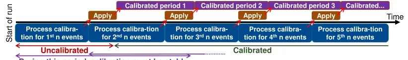
Figure1illustrates the online calibration scheme. The steps are processed in a pipeline, such that while the calibration result is fed back (Step B, brown) and then used in the reconstruction (Step C, purple), a new calibration is computed in parallel (Step A, blue). Accordingly, the reconstruction is not calibrated for events recorded at the very beginning of a run before Step B finishes. The final reconstruction objects stored at the end of the process for offline use are valid for all events, also those at the beginning. This scheme is feasible as long as the total time of steps A, B, and C is below the stability interval, e. g. 15 minutes in case of the TPC drift time calibration.
Time
Process calibra-tion for 1st n events
Process calibra-tion for 2nd n events
Process calibra-tion for 3rd n events
Process calibra-tion for 4th n events
Process calibra-tion for 5th n events
Apply Apply Apply Apply
Calibrated period 1
Start of
run Calibrated period 2 Calibrated period 3 Calibrated...
Uncalibrated Calibrated
During this period, calibration must be stable
Figure 1.Illustration of the online calibration scheme. The blue boxes are the intervals where the calibration data is aggregated. Afterwards there is a short delay to prepare new TPC transformation maps based on the calibration and distribute them in the cluster (brown box). Finally, the HLT reconstruction uses the calibration as long as it is stable (purple box).
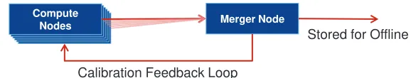
Naturally, a single instance of the calibration software running on a single processor cannot com-pute the calibration objects in time. The HLT runs the calibration component on 172 of its 180 computing nodes with 3 instances of the calibration per computing node, for a total of 516 calibration processes running in parallel. These instances process the incoming events in a round-robin fashion and regularly send their calibration data to a single calibration merger process running on a dedicated calibration computing node. This calibration node merges all the calibration data and creates the final calibration objects. The objects are stored for offline use and shipped back in parallel to all computing nodes by the feedback loop, such that the computing nodes can perform the reconstruction based on the new calibration. Figure2illustrates the process.
1The TPC cluster transformation map is needed to convert the raw TPC clusters from TPC pad row, TPC pad, and time
Compute
Nodes Merger Node
Stored for Offline
Calibration Feedback Loop
Figure 2.Illustration of the merging of calibration objects.
2.1 Requirements for online calibration
On top of the time constraints from the above approach, online calibration poses a couple of require-ments on the reconstruction and data transport framework, which are discussed in the following. This subsection concludes with a list of requirements that needed to be solved to run the TPC drift time calibration in the ALICE HLT. The following sections show how ALICE deals with these challenges. The custom data transport framework in the HLT can be seen as a directed graph. The fibres from the detector are input nodes in the graph, the network connections to the data acquisition (DAQ) are output nodes, and the remaining nodes in the graph are processing components. The links in the graph define the data flow. All processing components process the events in an event-synchronous way, i. e. they process one event after another in a pipeline. Long-running tasks as needed for the calibration pose a problem, because they stall the pipeline during the processing of the event. All processing components which are upstream of the stalled process become stalled as well as soon as the buffers run full. Another issue is that the HLT processing chain must be loop-free for technical reasons by design, because of the event-synchronous approach. A loop in the graph would impose a cyclic dependency, i. e. two processing components would wait for each other to finish processing the same event.
The TPC drift time calibration matches tracks reconstructed in the TPC to tracks in the ITS. This means the HLT must at least provide track reconstruction for the TPC and the ITS. On top of that, the track reconstruction in these detectors should be standalone, i. e. independent of each other, in order to avoid introducing a bias. Although the ITS delivers significantly less data than the TPC, tracking in the ITS is computationally intensive because of combinatorics, as the ITS sits in the center of ALICE where the track density is the highest. Also, the treatment of scattering in the silicon layers is more complicated than inside the gas volume of the TPC. Finally, ITS tracks have only up to six hits compared to more than 100 in the TPC, which requires a much more robust seeding procedure in order to find all tracks. Therefore, the default HLT method for ITS tracking is to prolong TPC tracks into the ITS and then collect the ITS hits close to the extrapolated tracks. This poses two problems: first, it could introduce a bias to use prolonged TPC tracks for the calibration of the TPC. Second, the prolongation into ITS where the track density is very high requires high precision and works well only if the TPC is calibrated. This leads to a chicken and egg problem.
Usually, calibration is performed relative to a default calibration. For instance, the TPC measures the clusters in row, pad, and time coordinates which must be transformed into spatial coordinates in order to run the track reconstruction and then the calibration. This transformation is performed using the initial, default calibration. The calibration uses the transformed clusters, and the exact transformation that was used to obtain the spatial coordinates of the clusters has an impact on the calibration output. In other words, the calibration must run on clusters transformed according to the default calibration, but not on calibrated clusters.
The following list summarizes the requirements for online calibration of the TPC drift in the ALICE HLT:
• Fast reconstruction algorithms for ITS and TPC.
• Independent standalone tracking algorithms for ITS and TPC. • Support for long-running tasks in the HLT framework. • Support for loops in the HLT data flow.
• Data structures enabling fast data exchange between processing components.
• The feedback loop must apply the calibration only to the tracking, but not to the calibration compo-nent.
• Calibration process and feedback loop must not take longer than the time interval during which the calibration remains stable.
2.2 Framework improvements
Adding the feedback loop directly to the loop-free HLT processing chain is a major architectural change. We wanted to avoid this since the current HLT data transport is thoroughly tested and we pre-ferred incremental changes. In particular, we prefer adding additional processing or communication components over changing the basis of the framework. Considering the general approach to online cal-ibration in the HLT, the calcal-ibration does not need to be event-synchronous. The calcal-ibration result is not fed back to the reconstruction of the same event, but at some later point in time. This can happen asyn-chronously. The HLT uses additional source and sink components based on the ZeroMQ data transport library for new communication channels not foreseen in the original framework [4, Subsection 5.3].
3 Track reconstruction in the TPC
The HLT employs GPU-accelerated track reconstruction for the ALICE TPC that is based on a Cellu-lar Automaton principle to build track seeds, i.e. short track candidates of around 5 to 10 hits. It then uses the Kalman filter for track fitting and track following [5,6]. The HLT employed 64 NVIDIA Geforce GTX480 GPUs during LHC Run 1. The new HLT farm for LHC Run 2 is now equipped with 180 AMD FirePro S9000 GPUs. One major concern with the original GPU tracker code was that it was based exclusively on the NVIDIA CUDA framework and was thus vendor-dependent. For Run 2, an OpenCL implementation was created, which uses the AMD OpenCL C++kernel language extensions. The code is written in a generic way, such that the same source code can be used with CUDA, OpenCL, and also for the CPU [4, Section 4]. This gives the greatest possible flexibility for hardware selection and reduces the maintenance effort.
Parallelization is implemented such that during the Cellular Automaton phase, one GPU thread handles one TPC cluster. During the track following, one GPU thread handles one TPC track. This allows for simple and efficient parallel processing, as the threads can operate almost fully indepen-dently. Considering the amount of TPC clusters and tracks in a typical Pb-Pb event as well as the number of threads a GPU executes concurrently, this scheme resulted in full GPU utilization at the time it was implemented, e. g. for the GTX480 GPUs during Run 1. Naturally, pp events with much fewer tracks do not use the GPUs efficiently. This is no problem however, as the GPUs are fast enough for pp reconstruction anyway. In the meantime, the number of threads a GPU needs to execute in par-allel to achieve full performance has increased significantly. The number of tracks increased only slightly when the LHC moved from 3.5 TeV/Zto 6.5 TeV/Zin Run 2. Overall, we see that now even single central Pb-Pb events are unable to load the S9000 GPUs of Run 2 to the full extent. Looking ahead to Run 3, this problem becomes even more severe because new GPUs will feature even more parallelism.
The maximum data rate the TPC can deliver to the HLT is defined by the number of optical links times the link speed. The HLT was tested with data replay at this maximum possible speed and was proven to be able to run the full TPC reconstruction, while still retaining some margin to run reconstruction for other detectors. Thus, development of HLT TPC track finding for Run 2 is complete. Now, the focus lies on testing improvements for the Run 3 online computing facility already in the HLT during Run 2.
As a first step, we increase the parallelism by processing multiple events on one GPU concurrently. While during the implementation of the first GPU tracker version, GPUs could only execute one kernel at a time, modern GPUs can execute many independent kernels, even from different host applications, in parallel. The HLT can run several instances of the tracker on one GPU processing multiple events concurrently, as long as there is enough GPU memory, which in case of Run 2 is sufficient for 3 central Pb-Pb events with pileup. Table1shows a first result. Naturally, the wall time for a single event increases, which is not relevant. (For reference, the time between a central Pb-Pb event reaches the HLT input until it leaves the HLT is in average around 3 seconds.) In contrast, the processing throughput increases by 31.8 %. Using all computing nodes at full capacity, the HLT can reconstruct 40 million TPC tracks per second.
approach is already shown by the track reconstruction in the current HLT, which processes the TPC sectors individually but concurrently, and merges the tracks segments afterward [5].
Another foreseen development for Run 3 is the porting of additional online reconstruction com-ponents on the GPU, in particular, because modern GPUs can execute multiple kernels at the same time. Canonical candidates for GPU adaptation are the ones before and after the GPU track finding in the HLT reconstruction chain (see Fig.7in the last section). As a first prototype, the final track refit, a sub-step of the TPC track merger and track fit component that merges the track segments re-constructed by the GPU track finding was ported to GPUs. The prototype needs in average 6.8 ms per event for the refit compared to 125.5 ms on a single CPU Core (Intel Nehalem 2.8 GHz, the same events as in Table1). The bottleneck in this case is the PCI Express transfer, which takes longer than the computation itself. Therefore, the most reasonable approach is to bring multiple successive components of the HLT chain onto the GPU, such that the data need not be transferred back and forth in between.
We plan to implement every new GPU processing component using a generic shared source code for CPU and GPU, in the same way as for the TPC tracking. In addition, the implementations should be flexible enough to be applicable in the new software framework for online computing in Run 3 but also in the current HLT framework. This will allow us to test new developments and benefit from them already in Run 2.
4 Track reconstruction in the ITS
4.1 Scheme of ITS tracking in the HLT
The initial ITS tracking in the HLT which starts from prolonged TPC tracks is unsuited for online calibration. Conversely, a full standalone ITS tracking has to deal with the excessive combinatorics inside ITS and would need too many CPU resources. The HLT thus employs a hybrid approach with two independent ITS tracking branches. The first is the traditional chain with prolonged TPC-ITS tracks. In order to ensure good tracking results, the TPC needs to be calibrated. In parallel, a second chain performs fast standalone ITS tracking that has some limitations. In particular, it is not required to have maximum efficiency, i. e. it does not need to find all tracks. It only needs to find sufficiently many tracks for the ITS–TPC matching in the calibration and for the luminous region estimation (see Section4.3). The scheme is visualized in Fig.3. The following subsection describes the ITS standalone tracking in the HLT.
4.2 Fast ITS standalone tracking
The aim of the online ITS standalone reconstruction is to provide a sample of primary ITS tracks sufficient for calibration, without attempting to maximize the track-finding efficiency. Instead, the emphasis is put on the processing speed and correctness of the tracking (minimization of random clusters attached to tracks). The algorithm uses as an input the ITS clusters from all six layers and
Table 1.Tracking time of HLT TPC GPU tracking processing two events in parallel, averaged over a selection of central Pb-Pb events.
Number of events Time Time per event
1 145 ms 145 ms
TPC Links
ITS Links
TPC Tracking
TPC / ITS Tracking
ITS standa- lone tracking
ESD Creation With calibrated TPC
Without calibration
Figure 3. Scheme of ITS tracking in the HLT with two branches. The lower branch runs the ITS standalone tracer providing ITS tracks in any case. The upper branch uses TPC to ITS prolongation resulting in a higher efficiency, but it needs a calibrated TPC in order to achieve reasonable resolution.
the primary vertex provided by the HLT components running upstream. The latter is obtained as the position to which the maximum number of vectors connecting the two innermost ITS layers (silicon pixel detectors, SPD) converge. The track reconstruction starts by rebuilding these vectors (track-lets), i. e. finding pairs of SPD clusters seen under nearly the same angle from the vertex point. The procedure is the optimized version of the off-line tracklet finding described in [7].
At the following step the tracks are found by following the tracklets to ITS layers at larger radii, where the ITS Silicon Drift and Strip Detectors (SDD and SSD, respectively) are . For every tracklet a Kalman filter is initialized by the momentum estimated from the vertex and a pair of SPD clusters. It is propagated outwards starting from the vertex, considered as a measured point. The Kalman prediction/update is done first with already attached SPD clusters, then on the SDD and SSD clusters closest to extrapolation point, provided they meet a strict track-to-clusterχ2cut. The magnetic field is taken to be a constant solenoidal one, an approximation correct to ≈ 10−3 in the ITS volume. Multiple scattering is accounted for using the average material budget per layer. At least four clusters are required per track in the reconstruction in standard layout with all six ITS layers present. Tracks with two consecutive layers without contribution are rejected. Once the outermost layer is reached, the trackoutward kinematics is recorded (for the further matching with TPC) and inward Kalman propagation is performed to obtain the kinematics at the vertex region.
The benchmark with simulated In pp and p-Pb events, on a single core of i7-2600 CPU @ 3.40 GHz, shows a rate obove 2 kHz with a reconstruction efficiency (with respect to reconstructable Monte Carlo tracks) exceeding 90% at pT > 300 MeV/cand a contamination by fake tracks below
3%. Minimum bias Pb-Pb events are reconstructed at a 18 Hz rate, which rises to 40 Hz if 15% of the most central collisions are skipped. The efficiency above pT >300 MeV/cdrops to about 85%, and
the fake rate is below 10%.
4.3 Luminous region estimation based on ITS tracking
The vertex determination is implemented in the same component that performs the ITS standalone tracking. First the tracks are propagated to the beam-line, then a fast linear fitter is deployed to find a vertex as a point minimizing the distance of the closest approach for maximum number of tracks. The rejection of outlier tracks is achieved by means of bi-square weighting filter, as described in [8].
5 Data structures for fast data transport in the HLT
5.1 A flat data structure
As discussed in Section2.1, one of the crucial features of the calibration procedures running in the HLT is the fact that they use the same code as used in the offline calibration. This was developed to work on the output of the offline reconstruction, i. e. on the C++structures called Event Summary Data (ESD) on which the ALICE analyses are based. The ESDs are not suited to be used in the HLT framework since the multiple processes that may run in the HLT do not share the same address space. This implies that shipping C++ objects (possibly in the form of ROOT objects) between HLT processes can be done only through serialization and deserialization, which would introduce an unacceptable overhead in the framework for every process that accesses the ESDs. The problem that arises when tasks that take as input the standard ESDs when run offline (e. g. calibration tasks, Quality Assurance, analysis...) are run in the HLT, can be overcome by storing the output of the HLT reconstruction in flat structures, which are exchanged between the different HLT reconstruction, calibration, and QA components complying with the HLT framework requirements.
The development and implementation of the flat ESDs is based on the C++concepts of inheritance and polymorphism. A common base class for the flat ESDs and the standard ESDs allows to run the same calibration algorithm online in the HLT and offline.
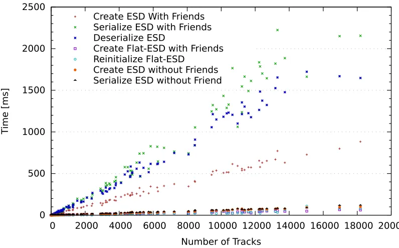
While in the ESDs the different objects that come out of the reconstruction are stored inside the ESDs as different C++objects, in the flat ESDs they are simply stored consecutively in memory, and the bookkeeping of their position in the object is used to access them. One special case among these objects is the so-called ESD friends, which is an object meant to store information not needed for analysis, but specifically for calibration. For example, it contains the information about the clusters used to form the tracks. Since every track can have up to 159 clusters associated in the TPC (due to the same number of pad-rows in the detector), the amount of data in the friends is very large, and the size of the friends can be several times the one of the ESD tracks.
5.2 Benchmarks
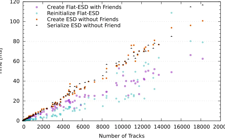
of the standard ESDs without the friends compared to the flat structure is better visible in Fig.5: also in this case the flat structures with the complete calibration information are more performant.
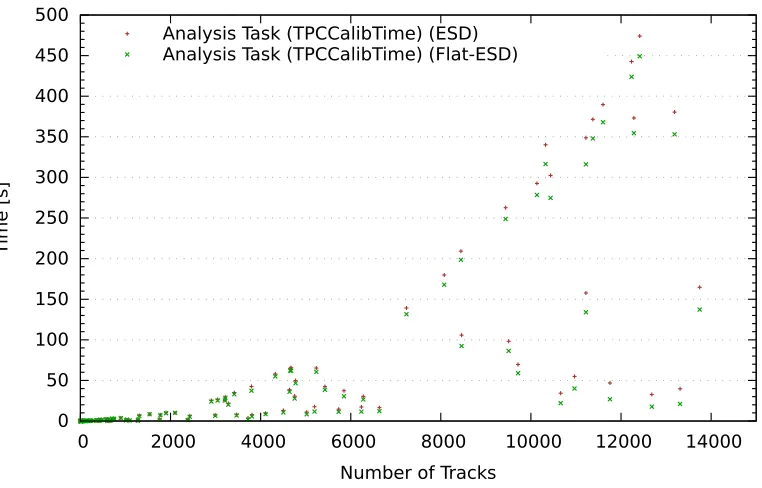
Figure6shows the time needed by the TPC drift time calibration task when running on standard ESDs and on flat ESDs. As one can see, the task performance is comparable when using as input the standard ESDs or the flat ones, being a few percent faster in case of the flat ESDs at high multiplici-ties. This is an additional minor advantage of the flat ESDs. The main advantage of the flat structures lies in the speed with which they are created and can then be shipped between different HLT compo-nents, more than in how fast they can be processed by the calibration task. This is anyway running asynchronously with respect to data taking, and as such it does not impose any performance limitation.
Table2 summarizes the resources needed to create the standard ESDs and the flat ESDs (with and without friends) in the HLT in number of CPU cores. Considering the total amount of resources available in the HLT cluster, i. e.≈2000 CPU cores, one realizes immediately that while the creation of standard ESDs as natural output of the HLT reconstruction is an expensive but well affordable process, adding the extra information needed to perform calibration tasks—i. e. what is stored in the friends—would require half of the total HLT resources, which is completely infeasible. In opposite, the flat ESDs can be created in the HLT together with the extra calibration data using a limited amount of resource, which is even smaller than those needed to generate the standard ESDs without friends.
0 500 1000 1500 2000 2500
0 2000 4000 6000 8000 10000 12000 14000 16000 18000 20000
T
ime [ms]
Number of Tracks Create ESD With Friends
Serialize ESD with Friends Deserialize ESD
Create Flat-ESD with Friends Reinitialize Flat-ESD
Create ESD without Friends Serialize ESD without Friend
Table 2.Number of CPU cores required to create normal and flat ESDs with and without friends obtained processing Pb-Pb (from 2015) events at 300 Hz.
ESD Type with/without friends Number of CPU cores
ESD Converter without friends 94.7
ESD Converter with friends 947.0
Flat-ESD Converter without friends 11.0
Flat-ESD Converter with friends 72.4
6 Overview of HLT online calibration and a first online calibration test run
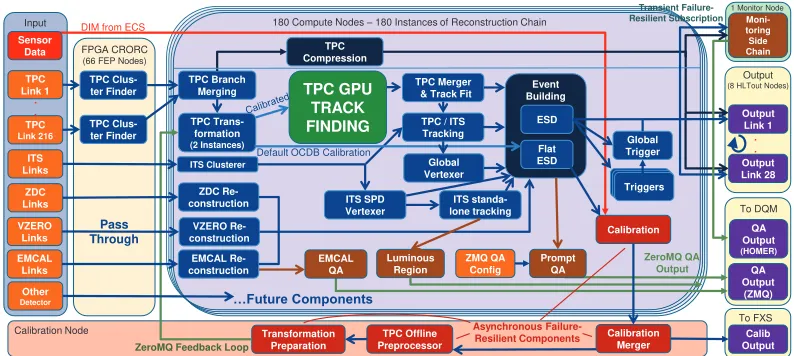
Figure7gives an overview over the data flow and all components in the HLT. The actual components used for online calibration are shown in red, and they use the new asynchronous processing feature. The actual calibration component is the only one that runs with many instances on all computing nodes. There is only one instance of the merger and the preprocessors, running on a dedicated calibration node. Then, the new TPC transformation maps based on the new calibration is distributed in the cluster via ZeroMQ. In order to make sure that the calibration component does not run on calibrated clusters, the TPC transformation component runs two instances. One uses the new transformation map from the feedback loop. The clusters from this instance are shipped to the tracker component. The other instance uses always the default transformation map and ships the clusters to the ESD, from where they go to the calibration component. The calibrated clusters in the tracks and the uncalibrated clusters for the ESD friends are identified via the cluster index which is unchanged
0 20 40 60 80 100 120
0 2000 4000 6000 8000 10000 12000 14000 16000 18000 20000
T
ime [ms]
Number of Tracks Create Flat-ESD with Friends
Reinitialize Flat-ESD Create ESD without Friends Serialize ESD without Friend
0 50 100 150 200 250 300 350 400 450 500
0 2000 4000 6000 8000 10000 12000 14000
T
ime [s]
Number of Tracks Analysis Task (TPCCalibTime) (ESD) Analysis Task (TPCCalibTime) (Flat-ESD)
Figure 6.Time needed for different steps in the creation and manipulation of the standard (without friends) and flat ESDs as a function of the track multiplicity of the event, obtained processing Pb-Pb (from 2015) events.
by the cluster transformation. Thus, the feedback loop improves the track finding, but does not interfere with the calibration itself.
Therefore, all the requirements of online calibration in the HLT listed in Section2.1are met. A first test of the above-described new features with online calibration was performed in December 2015. The calibration components were running online under real conditions during Pb-Pb data taking in ALICE at LHC design luminosity. This test proved that the HLT can handle the online calibration in a high load scenario with the highest data rates.
TPC Link 1 TPC Link 216 TPC Clus-ter Finder ITS Links . . ZDC Re- construction Output Link 1 Output Link 28 Event Building Calibration Sensor Data TPC Branch Merging TPC Trans-formation (2 Instances) Input FPGA CRORC (66 FEP Nodes)
ZDC Links VZERO Links EMCAL Links
DIM from ECS
TPC GPU TRACK FINDING
TPC Merger & Track Fit
TPC / ITS Tracking ITS standa- lone tracking ESD Flat ESD VZERO Re- construction EMCAL Re- construction . . QA Output (ZMQ) Luminous Region Prompt QA EMCAL QA TPC Clus-ter Finder
180 Compute Nodes ± 180 Instances of Reconstruction Chain
Calibration Merger Calib Output TPC Offline Preprocessor Transformation Preparation ZeroMQ QA Output
ZeroMQ Feedback Loop
Output
(8 HLTout Nodes)
Calibration Node TPC Compression Global Trigger Other Detector QA Output (HOMER) Moni-toring Side Chain
Default OCDB Calibration
Pass Through
«)XWXUH&RPSRQHQWV
To DQM
To FXS
1 Monitor Node
Triggers Triggers Triggers ITS SPD Vertexer Global Vertexer ITS Clusterer Asynchronous Failure- Resilient Components Transient Failure- Resilient Subscription ZMQ QA Config
Figure 7.Overview of all processing components and data flow in the HLT.
References
[1] A. K. et al. (ALICE Collaboration), JINST3, S08002 (2008)
[2] C. Fabjan et al. (ALICE Collaboration),ALICE trigger data-acquisition high-level trigger and control system: Technical Design Report, ALICE-TDR-10; CERN-LHCC-2003-062 (CERN, Geneva, 2004),https://cds.cern.ch/record/684651
[3] Facility for Antiproton and Ion Research in Europe Gmb,FAIR - Baseline Technical Report, Vol. 1 (2006), ISBN 3-9811298-0-6,
http://www.fair-center.de/index.php?id=171&L=0
[4] D. Rohr et al., J. Phys. Conf. Ser.664, 082047 (2015) [5] S. Gorbunov et al., IEEE Trans. Nucl. Sci.58, 1845 (2011) [6] D. Rohr et al., J. Phys. Conf. Ser.396, 012044 (2012)