The effect of statistical error model formulation on the fit and selection of mathematical models of tumor growth for small sample sizes

(1)

The effect of statistical error model formulation on the

fit and selection of mathematical models of tumor

growth for small sample sizes

H.T. Banks, Kidist Bekele-Maxwell, Judith E. Canner,

Amanda Mayhall, Jennifer Menda, and Marcella Noorman

Center for Research in Scientific Computation

Department of Mathematics

North Carolina State University

Raleigh, NC 27695-8212

and

Department of Mathematics and Statistics

California State University, Monterey Bay

Seaside, CA 93955

November 12, 2017

Keywords: Tumor growth models, mathematical and statistical models, sensitivity, complex-step method, residual analysis

(2)

Abstract

(3)

1 Introduction

Some standard and simple mathematical models are commonly used in tumor growth mod-eling and prediction studies ([8, 12, 13, 18, 22, 20, 24, 25]). A rather striking commonality in most of these studies is the small longitudinal nature (i.e., in terms of the duration and number N of observations or time points) of the data sets employed for model validation.

Our primary goal is to better understand statistical error models that arise in the obser-vation process for tumor data collection. As explained in [4, 7] and below, in order to verify and select the best mathematical model, the choice of an appropriate statistical error model is critical. In this study, we examine how the choice of statistical error model (and hence the form of least squares employed in the inverse problem) affects the accuracy and uncertainty of the mathematical model fits to data. We investigate this in a selection for tumor growth data from studies on mice with a small number of sampling observations [8, 13]. Thus our effort can be considered a further step in the goals of the authors of [8] in their efforts to more fully understand the form of the observation errors in tumor data collection processes. In our study, we use the same suite of mathematical models as discussed in [8]. These are the logistic, Gompertz, power law, exponential linear, generalized logistic, dynamic carrying capacity, and Von Bertalanffy models summarized for completeness in Section 2.1 along with the data we have chosen to illustrate our efforts in Section 2.2. Using several sets of tumor growth data from [8] and [13], we estimate model parameters for the mathematical models via the inverse problem methodology summarized in Section 3. This methodology includes the complex-step approach to sensitivity and standard error (SE) computation, residual analysis, second order differencing applied directly to the data, and Akaike-based information criteria selection procedures. In Section 4 we study the model solutions and the precision of the parameter estimates to investigate how the choice of the statistical error model affects the results of the mathematical models. Moreover, we estimate model parameters using a family of statistical error models and use various computational tools to determine the ones appropriate for such data sets. Finally in Section 4.4 we use Akaike information criterion (as introduced in Section 3.3) in attempts to rank order our models with the various data sets. We conclude in Section 5 with our conclusions and suggestions.

2 Models and Data Sets

2.1 Review of tumor growth models

(4)

2.1.1 Logistic model

The Logistic model is given by

(

dV

dt =aV 1−

V K

, t >0, V(0) =V0,

whereV represents tumor volume, a is the growth rate, andK is the carrying capacity. The analytic solution is given by

V(t) = KV0e

at

K+V0(eat−1)

.

The parameters of interest in fitting this model to data are θ = (q, V0) = (a, K, V0).

2.1.2 Gompertz model

The Gompertz model is given by

(

dV

dt =ae

−βt_V, _{t >}₀

V(0) =V0,

where V represents tumor volume, a is the growth rate, and β is the rate of exponential decay of the growth rate. The analytic solution is given by

V(t) =V0e

a β(1−e

−βt₎

.

The parameters of interest in fitting this model to data are θ = (q, V0) = (a, β, V0).

2.1.3 Generalized logistic model

The generalized logistic model is given by

(

dV

dt =aV 1−

V K

ν

, t >0, V(0) =V0,

where V represents volume, a is the growth rate, K is the carrying capacity, and ν is a constant. When ν = 1 we have the logistic model, whereas when ν > 1 the model demonstrates an exponential growth curve and decelerates quickly as K is maximized [22]. The analytic solution of the system is given by

V(t) = KV0 (Vν

0 + (Kν−V0ν)e−aνt) 1/ν.

(5)

2.1.4 Dynamic carrying capacity model

The dynamic carrying capacity model is given by



 

 

dV

dt =aV log

K V

, t >0,

dK

dt =bV

2/3_, _{t >}₀_,

V(0) =V0, K(0) =K0,

(2.1)

where V represents tumor volume, a is the growth rate, K is carrying capacity, and b is the growth or decay rate of the carrying capacity. The parameters of interest in fitting this model to data are θ = (q, V0, K0) = (a, b, V0, K0).

2.1.5 Power law model

The power law model is given by

(

dV

dt =aV

µ_,

V(0) = V0,

whereV represents tumor volume, ais the growth rate, andµis the allometry volume factor. The analytic solution is given by

V(t) = at(1−µ) +V₀1−µ

1

1−µ_.

The parameters of interest in fitting this model to data are θ = (q, V0) = (a, µ, V0). Note

that the power law model is a special case of the Von Bertalanffy model below, in which we letb = 0.

2.1.6 Von Bertalanffy model

The Von Bertalanffy model is given by

(

dV

dt =aV

µ₋_bV,

V(0) =V0,

where V represents tumor volume,a is the growth rate, and b is the term corresponding to the loss of volume. The analytic solution is given by

V(t) =a

b +

V₀1−µ− a

b

e−b(1−µ)t

1

1−µ

.

(6)

2.1.7 Exponential linear model

The exponential linear model is given by



 

 

dV

dt =a0V, t≤τ, dV

dt =a1, t > τ,

V(0) =V0,

where V represents tumor volume, a0 is the exponential growth rate, and a1 is the linear

growth rate. The analytic solution is given by

V(t) =

(

V0ea0t t≤τ,

a1(t−τ) +V0ea0τ t > τ,

where τ = 1

a0 ln( a1

a0V0) when V(t) is continuously differentiable. The parameters of interest

in fitting this model to data are θ = (q, V0) = (a0, a1, V0).

2.2 Data Sets

Data from three different types of tumors were utilized in this work: breast, lung, and skin (HPV) tumors. The lung and breast tumor data were obtained from [8] and the HPV data came from [13]. All the data were collected in labs on mice and extracted from figures in [8, 13] using the data extraction tools Data Thief (Version III) and WebPlotDigitizer (Version 3.12) [19, 23].

2.2.1 Data Set Descriptions

For the lung tumor data, male mice were injected subcutaneously with Murine Lewis lung carcinoma after the cells were cultured in a high glucose DMEM. For the breast tumor data, human breast carcinoma LM2−4LU C+ _{was implanted into the mammary fat pads}

of female immunosuppressed mice. The day the cancer cells were injected/implanted was considered day 0 and subsequent measurements of the tumors were collected using calipers to subcutaneously measure the largest (L) and smallest (w) diameters of the tumor. Assuming an ellipsoid shape, the volume of the tumor was then calculated using the formula

V = π 6w

6_L.

Lung tumors were allowed to grow to a maximum volume of 1.5cm3 before the mouse was euthanized, resulting in data collected over a 4 to 22 day period with volumes ranging from 14−1492mm3_{. Two experiments were conducted on ten mice each, resulting in twenty lung}

tumor data sets. Breast tumors were allowed to grow to a maximum volume of 2cm3 before the mouse was euthanized, resulting in data collected over an 18 to 38 day period with volumes ranging from 202−1902mm3_{. Experiments were conducted on a total of 34 mice}

(7)

For the skin (HPV) tumors, mice were bred to carry E6/E7 double transgenes and treated with DMBA/TPA. Experiments were conducted on 8 mice. For each mouse, three tumors were randomly selected and measurements were taken biweekly resulting in twenty-four data sets for the skin (HPV) tumors. Measurements began when the tumor became visible (approximately 1−2mm in diameter) with day 0 set to the date of the first measurement. Each tumor’s length (x) and width (y) were measured three times using measuring calipers and the medians (Mx and My) of these measurements calculated. Assuming an ellipsoid

shape, the volume of the tumor was calculated using the formula

V = π

6(MxMy)

3/2_.

Skin tumors were allowed to grow to a maximum diameter of 1cm before the mouse was euthanized. Life spans of individual mice ranged from 42 to 105 days. Tumor size, at its largest, ranges from 295.55mm3 _{to 864}_._82mm3 _[13].

In this study, we examined all combinations of the proposed mathematical models and a selection of representative statistical models on a subset of tumors from each data set. We selected four mice of each tumor type to analyze the model fits and choice of statistical error model. We chose the following tumors to show how different models fit the data sets with varying dynamics:

1. Breast Tumors 15, 16, 31, and 33. Breast Tumor 15 (B15) has 8 data points and time

ranges from day 18 to day 34. Breast Tumor 16 (B16) has 8 data points and time ranges from day 18 to day 34. Breast Tumor 31 (B31) has 7 data points and time ranges from day 22 to day 36. Breast Tumor 33 (B33) has 8 data points and time ranges from day 22 to day 38.

2. Lung Tumors 2, 4, 5, and 9. Lung Tumor 2 (L2) has 11 data points and time ranges

from day 5 to day 20. Lung Tumor 4 (L4) has 12 data points and time ranges from day 6 to day 22. Lung Tumor 5 (L5) has 11 data points and time ranges from day 5 to day 20. Lung Tumor 9 (L9) has 10 data points and time ranges from day 6 to day 20.

3. Skin (HPV) Tumors 4, 9, 12, and 24. Tumor 4 (T4) has 23 data points and time

ranges from day 0 to day 76. Tumor 9 (T9) has 24 data points and time ranges from day 0 to day 88. Tumor 12 (T12) has 14 data points and time ranges from day 0 to day 52. Tumor 24 (T24) has 13 data points and time ranges from day 0 to day 42.

3 Components of Inverse Problem Studies:

Mathe-matical and Statistical Models

(8)

methodology of the inverse problem for the following general 1-dimensional dynamical model:

dx

dt(t) =g(t, x(t);q), x(t0) =x0,

with observation process

f(t;θ) =Cx(t;θ),

whereθ = [qT_{, x}T

0]T ∈Rκθ,q∈Rkq is a vector parameter and C is the observation constant.

Suppose we haveN longitudinal observations{Yj}(with realizations{yj}) corresponding

to f(tj;θ) = Cx(tj;θ), j = 1,· · · , N, and let Ωθ be the set of admissible parameters. In

general, {Yj} will not be exactly equal to f(tj,θ). To account for this uncertainty in the

observations, we use a statistical error model for the observation process given by

Yj =f(tj;θθθ0) +fγ(tj;θθθ0)Ej, j = 1,· · · , N, γ ≥0. (3.1)

Here,θθθ0 ∈Ωθ represents the “true” or nominal parameter set that generates{Yj} (assumed

to exist), and fγ₍_t

j;θθθ0)Ej represents the measurement error or some other phenomena that

causesYj 6=f(tj;θθθ0). We assumeEj are independent over time with mean zero and constant

variance.

Whenγ = 0, i.e., when the error has constant variance, the statistical error model (3.1) is called the absolute error model and we estimate the parameters by minimizing the ordinary least squares (OLS) cost function:

θOLS = arg min

θ∈Ωθ

N

X

j=1

(Yj −f(tj;θ))2,

with realization

ˆ

θOLS = arg min

θ∈Ωθ

N

X

j=1

(yj −f(tj;θ))2. (3.2)

Whenγ 6= 0, i.e., when the error has non-constant variance, we use an iterated reweighted weighted least squares (IRWLS) scheme to estimate the parameters. Note, whenγ = 1, the statistical error model is called therelative error model. We compute the parameter estimates by solving

θIRWLS= arg]min

θ∈Ωθ

N

X

j=1

1

f2γ₍_t j;θ)

(Yj −f(tj;θ))2,

wheremin denotes an iterative minimization scheme that is explained in Section 3.1.1. Note,g

this scheme is not equivalent to a traditional minimization. To obtain realizations ofθIRWLS,

we solve

ˆ

θIRWLS= arg]min

θ∈Ωθ

N

X

j=1

1

f2γ₍_t j;θ)

(yj−f(tj;θ))2. (3.3)

(9)

3.1 Computational methods

To fit the seven mathematical models to the data, we solve an inverse problem in each case to estimate model parameters. When an absolute statistical error model is used, we estimate ˆθOLS using Matlab’s built-in optimization solver fmincon directly to minimize the

cost function in (3.2). In the case when γ > 0, we use the numerical algorithm provided in [4, 6] to estimate ˆθIRWLS which is summarized below.

3.1.1 IRWLS algorithm

To compute ˆθIRWLS, we will make use of the weighted least squares cost functional:

ˆ

θ = arg min

θ∈Ωθ

N

X

j=1

wj(yj−f(tj;θ)) (3.4)

1. Solve for an initial estimate ˆθ0 by solving (3.2). Setl = 0. 2. Compute the weights wj =f−2γ(tj; ˆθ

(l)

).

3. Re-estimate ˆθ by solving (3.4) with the weights computed in step 2 fixed to obtain ˆ

θ(l).

4. If ˆθ(l) and ˆθ(l+1) are sufficiently close, set ˆθIRWLS= ˆθ (l+1)

. Otherwise, setl =l+ 1 and return to step 2.

All of the dynamical systems are solved using the Matlab ode45 ODE solver which is based on the fourth order Runge-Kutta scheme.

3.1.2 The complex-step method for computing sensitivities

There are numerous methods for computing sensitivities with respect to parameters in models such as those under consideration here. These are discussed in some detail in [4, 7] and include forward differences, sensitivity equations, traditional sensitivity functions (TSF), relative sensitivity functions (RSF), and automatic differentiation (see [4, p. 74-76]). Here we use a method based on analyticity of the functions involved [1, 2].

This method, referred to as the complex-step method, has gained some popularity in the engineering community in calculating sensitivities [16, 17]. The idea of using complex variables to estimate derivatives originated with the work of Lyness and Moler [15] and Lyness [14] for analytic functions where they used the Cauchy-Riemann equations in a crucial way. More recently the method was studied in [1, 2] and shown to be much more widely applicable. Indeed one can argue this since we have for any C2 _{function in} _θ_{, the 2nd order}

Taylor expansion using the complex step ih

f(t;θ+ih) =f(t;θ) +ih∂f

(10)

where

limR2(h)

h = 0.

Taking the imaginary parts of both sides and dividing by h in (3.5) results in the first order approximation

∂f

∂θ(t;θ) =f

0

(t;θ)≈ Im[f(t;θ+ih)]

h (3.6)

with a truncation errorET approximated by

ET(h)≈

h2

6

∂3_f

∂θ3(t;θ).

Terms of order h2 _{and higher can be ignored because the step size} _h _{can be chosen}

up to machine precision. The method is accurate down to a specific step size we can call

hcrit. Below hcrit, underflow occurs and the approximation becomes useless. This derivative

estimate constitutes a big advantage over other approximation approaches to sensitivities. First, it is applicable for problems with less smoothness than analyticity (e.g., functions only C2 in the parameters). Moreover, usual finite-difference approximations are subject

to subtractive error due to the differencing operation. On the other hand, the accuracy of

the complex-step estimates is only limited by the numerical precision of the algorithm that evaluates the function f.

3.1.3 The complex-step method: implementation

General steps for implementing the complex-step method for computing df /dxare

1. Define all functions and operators that are not defined for complex arguments. For example max, min and abs.

2. Add a small complex stepihto the desired variablex, run the algorithm that evaluates

f.

3. Compute df /dxusing _dxdf ≈ Im[f(x_h+ih)]

3.1.4 Computation of standard errors

Absolute error: We compute the sensitivity matrix

χj,k =

∂f(tj,θˆ)

(11)

which is done using the complex-step method as detailed above and in [1]. Note thatχ=χN

is an N ×κθ matrix. The constant variance is estimated by

ˆ

σ2 = 1

N −κθ

" _N X

j=1

[yj −f(tj,θˆ)]2

#

.

The covariance matrix is approximately given by

ΣN₀ ≈σ2₀χT(θ0)χ(θ0)

−1

,

and the approximate Fisher Information Matrix (FIM) is given by

F = (ΣN₀ )−1. (3.8)

As θ0 and σ20 are unknown, the covariance matrix is estimated by

ˆ

ΣN(ˆθ) = ˆσ2

χT(ˆθ)χ(ˆθ)−1

, (3.9)

for which the corresponding estimate of the FIM is

ˆ

F = ( ˆΣN(ˆθ))−1 = 1 ˆ

σ2

χT(ˆθ)χ(ˆθ). (3.10) Then, the asymptotic standard errors are estimated by

SEk(ˆθ) =

q

( ˆΣN_(ˆ_θ₎₎

kk, k = 1, . . . , κθ. (3.11)

Relative error: For the generalized weighted least squares formulations (IRWLS) used

here, we may define the standard errors by the formula

SEk=

q

ˆ ΣN

kk(ˆθ), k= 1, ..., κθ,

where the covariance matrix ˆΣN _{is given by}

ˆ

ΣN(ˆθ) = ˆσ2(χT(ˆθ)W(ˆθ)χ(ˆθ))−1 = ˆσ2Fˆ−1.

Here

ˆ

F =χT(ˆθ)W(ˆθ)χ(ˆθ) (3.12) is the Fisher Information Matrix defined in terms of the sensitivity matrix defined above and written compactly as

χ= ∂f

∂θ =

∂f(t1; ˆθ)

∂θ , . . . ,

∂f(tN; ˆθ)

∂θ

!

of size N ×κθ (recall N is the number of data points and κθ is the number of estimated

parameters) and the weight matrix W is defined by

(12)

We use the approximation of the variance given by

σ2₀ ≈σˆ(ˆθ)2 = 1

N −κθ N

X

i=1

1

f(ti; ˆθ)2γ

(yi−f(ti; ˆθ))2.

A quick comparison of (3.10) and (3.12) reveals that the uncertainty calculations will

be invalid if one chooses an incorrect statistical error model to compute the

correspond-ing standard errors. This of course also affects directly the calculations of the estimates themselves.

3.2 Methods for selection of a statistical error model

Before estimating model parameters, one should make efforts to determine the correct sta-tistical error model to account for the uncertainty of the data (such as observation error). We note that a misspecified statistical error model can lead to an incorrect estimation of the parameters as well as their uncertainly bounds. With the assumption on the errors Ej

(i.e.,i.i.d, mean zero, and constant variance) in the previous section, there are generally two ways of selecting the correct statistical error model, namely, using residual plots or apply-ing second-order differencapply-ing techniques directly to the data [3, 4]. We briefly discuss these methods below. More details can be found in [3, 4].

3.2.1 Residual plots

Calculating residual plots after performing an inverse problem is a common method to determine the appropriate statistical error model. Given the assumed statistical error model (3.1), for j = 1, . . . , N, residuals/modified residuals are defined by

rj =



   

   

yj −f(tj; ˆθ), γ = 0

yj −f(tj; ˆθ)

f(tj; ˆθ)γ

, γ 6= 0.

Note that rj is an approximate realization of Ej. Under the assumption of independence,

one can conclude that the residual plot of rj vs. tj will appear random. If Ej have constant

variance, the residual plot rj vs. f(tj; ˆθ) will be random. Residual plots with distinct

trends such as increasing or decreasing behavior, or fan-like shape indicates the assumptions of constant variance and/or independence is incorrect. One should then re-evaluate the statistical error model selection.

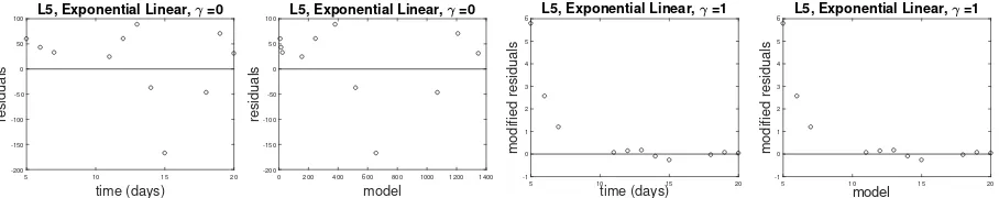
Several sample residual plots are given below in Figs 1-3 for different combinations of tumors, statistical error models, and mathematical models. Due to the small sample size in the breast, lung, and HPV tumor data sets, it is difficult to claim one residual plot is more random than another, as seen in the residual plots for the breast tumor logistic model for

(13)

regards to Ej are made, such as for the lung tumor fitted by the exponential linear model

when γ = 1 residual plot in Fig. 2. Moreover, this trend is found in all of the lung tumors among all of the mathematical models for the statistical error model whenγ = 1. In general, though, there is rarely a consistent pattern for the selection of a specific statistical error model based on the residual plots for each tumor type and mathematical model, as seen in Fig. 3 for the power law model fit to an HPV tumor data set forγ = 0,0.25,0.5,0.75,0.84,1. Thus the selection of γ based on the residual plots is inconclusive due to sparsity of data.

1. Sample residual plots for a selected breast tumors

18 20 22 24 26 28 30 32 34

time (days) -60 -40 -20 0 20 40 60 residuals

B15, Logistic, =0

200 400 600 800 1000 1200 1400

model -60 -40 -20 0 20 40 60 residuals

18 20 22 24 26 28 30 32 34 time (days) -0.15 -0.1 -0.05 0 0.05 0.1 0.15 0.2 modified residuals

%15, Logistic, =1

200 400 600 800 1000 1200 1400

model -0.15 -0.1 -0.05 0 0.05 0.1 0.15 0.2 modified residuals

Figure 1: Residuals and modified residuals for breast tumor B15 for γ = 0 & 1 using the Logistic model

2. Sample residual plots for a selected lung tumors

5 10 15 20

time (days) -200 -150 -100 -50 0 50 100 residuals

L5, Exponential Linear, =0

0 200 400 600 800 1000 1200 1400

model -200 -150 -100 -50 0 50 100 residuals

5 10 15 20

time (days) -1 0 1 2 3 4 5 6 modified residuals

5 10 15 20

model -1 0 1 2 3 4 5 6 modified residuals

(14)

3. Sample residual plots for a selected HPV tumors

0 10 20 30 40 50 60

time (days) -80 -60 -40 -20 0 20 40 60 80 residuals

T12, Power Law, =0

200 300 400 500 600 700 800 900 model -80 -60 -40 -20 0 20 40 60 80 residuals

0 10 20 30 40 50 60

time (days) -20 -15 -10 -5 0 5 10 15 modified residuals

T12, Power Law, = 25e-2

200 300 400 500 600 700 800 900

model -20 -15 -10 -5 0 5 10 15 modified residuals

T12, Power Law, = 25e-2

0 10 20 30 40 50 60

time (days) -0.2 -0.15 -0.1 -0.05 0 0.05 0.1 0.15 modified residuals

200 300 400 500 600 700 800 900 model -0.2 -0.15 -0.1 -0.05 0 0.05 0.1 0.15 modified residuals

0 10 20 30 40 50 60

time (days) -80 -60 -40 -20 0 20 40 60 80 residuals

T12, Power Law, = 84e-2

200 300 400 500 600 700 800 900 model -80 -60 -40 -20 0 20 40 60 80 residuals

T12, Power Law, = 84e-2

Figure 3: Residuals and modified residuals for HPV tumor T12 for γ = 0,0.25,0.84 & 1 using the Power Law model.

3.2.2 Second-order differencing techniques

To produce residual plots, one has to solve an inverse problem for each γ value. This could be computationally expensive. In addition, if the correct mathematical model is not used, residual plots could give inaccurate information, as these plots depend on the solution of the mathematical model. A method that relies only on the data itselffor identifying the correct observational statistical error model is asecond-order differencing technique and is described in detail in [3]. This method is found to be more accurate and efficient than using residual plots [3] as well as not requiringprior solution of inverse problems.

We first compute pseudo measurement errors ˆεj directly from the data {yj}Nj=1:

ˆ

εj =

                   1 √

2(yj+1−yj), j = 1 1

√

6(yj−1−2yj+yj+1), j = 2, . . . , N −1 1

√

2(yj−yj−1), j =N.

We then calculate the modified pseudo errors for different γγγ values. For, each data set, the modified pseudo error at time tj is defined as

ηj =

ˆ

εj

|yj−εˆj|γ

(15)

We attempted to use this second order differencing technique directly with several of our larger data sets, namely the HPV tumors. However, due to small sample size, our data sets again failed to yield useful information as to the appropriate statistical models to employ. Thus, even our larger data sets were too small to produce conclusive results for the correctness of statistical models.

3.2.3 Evaluation criteria

As neither of our proposed methods of choosing a statistical error model a priori yielded results for our small longitudinal data sets, we examine the effects of the choice of the statistical error model (γ values) on the performance of each mathematical model using four criteria: visual fit, standard errors (SEs), mean square errors (MSEs), and consistency of parameter estimates across γ values. When comparing visual fits, we look for discrepancies between the model fit and the data graphically. If there is little to no discrepancy, we conclude that it is a reasonable visual fit for the data. Standard errors of parameter estimates describe the uncertainty of the estimate. If the SEs of a particular parameter are on the same order of magnitude as the parameter estimate, there is a great deal of uncertainty in that parameter estimate. If the SEs are larger than the parameter estimate, the level of uncertainty in the parameter estimation is too high to draw reasonable conclusions. Mean squared error is a measure of how well the model fits the data. If the MSEs are consistent across statistical models and SEs for certain parameters are relatively large, we conclude that the model fits are not sensitive to those parameters. If MSEs vary across statistical models, we conclude that certain statistical models capture the dynamics of the data set more accurately than others. We examine the consistency of parameter estimates among the different statistical models to see if changing γ has an effect on the parameter values.

3.3 Methods for selection of a mathematical model

Once we have chosen an appropriate statistical error model, we compare mathematical mod-els using a model selection criterion, namely,the Akaike information criterion AIC. Assum-ing that the true mathematical model is known and the measurement errorsEj, j = 1,· · · , N

are independent and identically distributed with mean zero and constant variance σ2 _(see

Section 3), the AIC for univariate observations is given by

AIC =−2 lnL(ˆθ|y) + 2κθ,

where ˆθ is the estimate of θ using the appropriate statistical error model. Because our data set has a small sample size, we will usethe small sample Akaike information criterion AICc,

given by

AICc= AIC +

2κθ(κθ+ 1)

N −κθ−1

.

For the given statistical error model, the mathematical model with the smallest AICc is

(16)

4 Results

We fit seven mathematical models to three types of tumor data sets (breast, lung, and skin (HPV) tumors), and used γ values ranging from 0 to 1 for the the statistical error model (3.1). Specifically, we takeγ = 0,0.25,0.5,0.75,0.84,1. Whenγ = 0.84, we use the statistical error model as in [8]. This error model was chosen because, in practice, there is a threshold below which accurate measurements are not possible due to detectability limits. Benzekry et al. [8], experimented with different values and concluded that a threshold ofV = 83mm3

paired with γ = 0.84 gave an accurate description of error in the breast and lung tumor data. The HPV data set did not have a volume measurement below the threshold, thus the statistical error model given by (3.1) was used whenγ = 0.84 for the HPV data.

In keeping with conventions in [8], we first fixedV0 for the lung tumor data; however, we

subsequently chose not to fix V0 for the breast tumor data as we found that estimating this

parameter gave a more reasonable visual fit. The lung tumor data was plotted starting at day 0, the day of injection, with the initial condition V0 = 1mm3. The breast data set was

plotted starting at the day of first measurement, using the first measurement volume as the initial estimate. Originally we plotted the breast data starting at day 0, but because of the sparsity of the data, the linear dynamics, and relatively long time interval between day 0 and the first measurement day, we found that plotting using the first measurement day gave a more reasonable visual model fit. In contrast, the lung tumor data fit well visually using day 0 with the fixed initial condition because the first measurement day was much closer (in comparison to the breast data) to day 0.

In the exponential linear model for the lung data set, we provide parameter estimates for a0. However, we do not include a parameter estimate for a0 for the breast or the skin

data sets. This is because in both the breast and skin data sets, we start with a relatively large estimate of V0, rather than fixing V0 = 1mm3. WhenV0 is large,τ is either negative or

smaller than the first measurement day, forcing the model to be exclusively linear (section 2.1.7). Thus it is unnecessary to include the exponential growth rate parameter a0 as it is

not used in our model estimation. With a much largerV0, it is reasonable to have exclusively

linear growth, as the model implies that exponential growth occurs when the tumor is small (namely, below the τ threshold).

4.1 Visual inspection of the model fits

We summarize our findings for the various types of tumors based solely on visual fits to data.

4.1.1 Breast tumor data sets

(17)

the fit flattens out. When using the dynamic carrying capacity model, we see that the fits are overly sensitive to the second data point for most γ values in each of the four breast tumors and for B33 whenγ ≥0.84.Asγ increases, the weights on the smaller measurements also increase, which causes an overfit to the cluster of smaller measurements. The logistic, Gompertz, generalized logistic, and exponential linear models give consistently reasonable visual fits regardless of the choice of the statistical error model. In Figure 4, we display plots of the model fits for selected tumor data and γ values.

15 20 25 30 35

time (days) 0 500 1000 1500 Volume (mm 3)

Model Data

15 20 25 30 35

B16, Gompertz, = 25e-2

Model Data

20 25 30 35 40

B31, Generalized Logistic, = 50e-2

Model Data

20 25 30 35 40

B33, Dynamic C.C., = 84e-2

Model Data

20 25 30 35 40

B33, Power Law, =0

Model Data

20 25 30 35 40

B33, Power Law, =1

Model Data

20 25 30 35 40

B31, Von Bertalaffny, = 50e-2

Model Data

20 25 30 35 40

B31, Von Bertalaffny, = 75e-2

Model Data

Figure 4: Sample model fits of selected mathematical and statistical models for breast tumor data

4.1.2 Lung tumor data sets

When γ = 0.75 and γ = 0.84, the logistic model seems to reach a carrying capacity prema-turely; this is true for L2, L4, and L9. For the exponential linear model, when γ ≥ 0.75, the model fit becomes linear too soon, with a growth rate that underestimates the data in all four lung tumors. When γ = 1, the Gompertz and generalized logistic fit plots do not accurately represent the data for L4, L5 and L9. In the case of the Gompertz plots, the model fit underestimates the volume. For the generalized logistic, the model overestimates the volume. The dynamic carrying capacity, Von Bertalanffy, and power law models have consistent visual fits for all of the statistical models, respectively.

(18)

0 5 10 15 20 time (days) 0 500 1000 1500 Volume (mm 3)

L2, Logistic, = 75e-2

Model Data

0 10 20 30

L4, Gompertz, = 25e-2

Model Data

0 10 20 30

L4, Gompertz, =1

Model Data

0 5 10 15 20

L9, Generalized Logistic, =1

Model Data

0 5 10 15 20

time (days) 0 500 1000 1500 2000 Volume (mm 3)

L2, Power Law, =0

Model Data

0 10 20 30

L4, Von Bertalaffny, = 50e-2

Model Data

0 5 10 15 20

L5, Exponential Linear, = 75e-2

Model Data

0 5 10 15 20

L9, Dynamic C.C., = 75e-2

Model Data

Figure 5: Sample model fits of selected mathematical and statistical models for lung tumor data

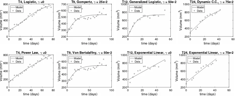
4.1.3 Skin (HPV) tumor data sets

Regardless of the statistical error model used, logistic, Gompertz, generalized logistic, dy-namic carrying capacity, power law, and Von Bertalanffy models produce consistently good visual fits for three of the four tumors in this data set, namely, T4, T12, and T24. The model fits for T9 exhibit large discrepancies between the model fit and the data due to the data’s extreme non-monotonic behavior. We note that all mathematical models are monotonic; the dynamics of the data are fairly sporadic and include an outlier, as seen in the following plots. The exponential linear model does not capture the dynamics of the data for T9 and T12, but gives a better visual model fit for T4 and T24. We assume this is because the latter two data sets exhibit a more linear behavior. In Figure 6, we display plots of the model fits for selected tumor data and γ values.

4.2 Parameter estimates, standard errors and mean squared

er-rors

(19)

0 20 40 60 80 time (days) 0 200 400 600 800 Volume (mm 3)

T4, Logistic, =0

Model Data

0 50 100

time (days) 200 300 400 500 600 700 Volume (mm 3)

T9, Gompertz, = 25e-2

Model Data

0 20 40 60

T12, Generalized Logistic, = 50e-2

Model Data

0 20 40 60

T24, Dynamic C.C., = 75e-2

Model Data

0 20 40 60 80

Model Data

0 50 100

time (days) 200 300 400 500 600 700 Volume (mm 3)

T9, Von Bertalaffny, = 50e-2

Model Data

0 20 40 60

T12, Exponential Linear, =0

Model Data

0 20 40 60

T24, Exponential Linear, = 75e-2

Model Data

Figure 6: Sample model fits of selected mathematical and statistical models for skin (HPV) tumor data

from each data set.

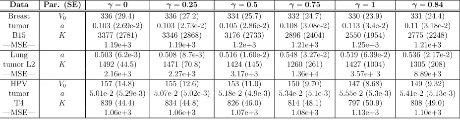
4.2.1 Logistic model

For the breast tumor data (excluding B33), the estimates for K vary as γ changes (9.26−

38.8% difference), however we also see large standard errors (75.5−382% of the estimate). This, along with the consistency of mean squared errors across different γ values (< 5% difference), suggests that the model fit is not sensitive to K. This is likely due to the lack of information in the data with regards to carrying capacity (i.e. data was not taken long enough for the carrying capacity to become apparent). A visual inspection of the breast tumor data further validates this assertion. The exception to this is B33. For this tumor, the standard errors are smaller (though still at 15.5− 23% of the estimate) however the difference in the estimates for K is only 0.81%. Further, in contrast to the other sets of breast tumor data, the B33 data set does visually suggest a possible carrying capacity.

For the lung tumor data sets, the standard errors are smaller relative to the estimate when

γ = 0 (1.28−2.47% fora and 2.98−12.4% forK) and largest whenγ = 1 (11.6−22.3% for

a and 70.4−169% for K). The large standard errors when γ = 1 may, in part, be due to the fact that the minimizer oscillated between two different parameter sets for this value of

γ. The size of MSE varies with γ (difference of 15.8−67%) though is consistently smallest when γ = 0.

There is no consistent discernable dependence upon γ for the HPV tumor data sets.

4.2.2 Gompertz model

(20)

Data Par. (SE) γ=0 γ=0.25 γ=0.5 γ=0.75 γ=1 γ=0.84

Breast V0 336 (29.4) 336 (27.2) 334 (25.7) 332 (24.7) 330 (23.9) 331 (24.4)

tumor a 0.103 (2.69e-2) 0.103 (2.73e-2) 0.105 (2.86e-2) 0.108 (3.08e-2) 0.113 (3.4e-2) 0.11 (3.18e-2)

B15 K 3377 (2781) 3346 (2868) 3176 (2733) 2896 (2404) 2550 (1954) 2775 (2248)

—MSE— 1.19e+3 1.19e+3 1.2e+3 1.21e+3 1.25e+3 1.21e+3

Lung a 0.503 (6.2e-3) 0.508 (8.7e-3) 0.516 (1.60e-2) 0.548 (3.27e-2) 0.519 (6.39e-2) 0.536 (2.17e-2)

tumor L2 K 1492 (44.5) 1471 (70.8) 1424 (145) 1260 (261) 1427 (1004) 1305 (208)

—MSE— 2.16e+3 2.27e+3 3.17e+3 1.36e+4 3.57e+ 3 8.89e+3

HPV V0 157 (14.8) 155 (12.6) 153 (11.0) 150 (9.70) 147 (8.68) 149 (9.32)

tumor a 5.01e-2 (5.29e-3) 5.07e-2 (5.02e-3) 5.18e-2 (4.9e-3) 5.34e-2 (5.1e-3) 5.55e-2 (5.3e-3) 5.41e-2 (5.13e-3)

T4 K 839 (44.4) 834 (44.8) 826 (46.0) 814 (48.1) 797 (50.9) 808 (49.0)

—MSE— 1.06e+3 1.06e+3 1.07e+3 1.08e+3 1.13e+3 1.10e+3

Table 1: Parameter estimates, SEs, and MSEs using the logistic model.

estimates, the percentage difference of estimates is 3−15% and the SEs are still ≥50% of the estimates. While MSE, for the most part, increases as γ increases, the change in MSE is always <6%. Thus, the inconsistency in parameter estimates for a and β is likely due to insensitivity.

For the lung tumor data, we see much larger MSE when γ = 1 and when γ = 0.75 for three of the lung tumors. In addition, SEs are smallest when γ = 0 and largest when

γ = 1,0.75. However, in contrast to the breast tumor data, SE’s are always <16%. We also don’t see nearly as much variability in parameter estimates for the lung tumor data, with percentage differences staying below 15%.

For the HPV data, we did not observe a notable quantifiable dependence uponγ. There are some instances when γ = 1 provides the smallest standard errors while γ = 0 provides the largest, however these instances are not sufficiently consistent over the data sets for us to draw any conclusions. Further, the percentage difference of the parameter estimates over

γ are all <4% and that of the MSE’s is <1%.

Breast V0 329 (51.7) 323 (45.8) 317 (40.3) 311 (35.2) 304 (30.3) 308 (33.4)

tumor a 0.115 (0.120) 0.136 (0.137) 0.165 (0.165) 0.212 (0.211) 0.289 (0.29) 0.235 (0.235)

B16 β 1.13e-2 (3.74e-2) 1.72e-2 (3.73e-2) 2.46e-2 (3.78e-2) 3.41e-2 (3.87e-2) 4.64e-2 (4.0e-2) 3.82e-2 (3.91e-2)

—MSE— 3.35e+3 3.36e+3 3.43e+3 3.60e+3 4.00e+ 3 3.71e+3

Lung a 0.566 (2.45e-2) 0.578 (2.76e-2) 0.597 (3.63e-2) 0.643 (5.10e-2) 0.728 (6.17e-2) 0.588 (3.12e-2)

tumor L4 β 5.58e-2 (5.2e-3) 5.84e-2 (5.9e-3) 6.25e-2 (7.7e-3) 7.24e-2 (1.10e-2) 9.07e-2 (1.34e-2) 6.07e-2 (7.0e-3)

—MSE— 1.59e+3 1.63e+3 1.86e+3 3.50e+3 1.20e+4 1.76e+3

HPV V0 254 (32.2) 255 (28.1) 256 (24.6) 257 (21.5) 258 (18.9) 257 (20.5)

tumor a 5.35e-2 (0.02) 5.26e-2 (0.018) 5.18e-2 (0.016) 5.09e-2 (0.015) 5.00e-2 (0.013) 5.06e-2 (0.014)

T9 β 7.15e-2 (1.87e-2) 7.07e-2 (1.76e-2) 6.98e-2 (1.66e-2) 6.98e-2 (1.56e-2) 6.89e-2 (1.48e-2) 6.86e-2 (1.53e-2)

—MSE— 1.86e+3 1.86e+3 1.86e+3 1.86e+3 1.864e+3 1.863e+3

Table 2: Parameter estimates, SEs, and MSEs using the Gompertz model.

4.2.3 Generalized logistic

For the most part, the standard errors for the estimates of a and ν are > 100% of the estimate itself. The exceptions are HPV tumor T4, for which the standard errors for a are 3.24−64.8% of the estimate, and lung tumor L2, for which the standard errors for a when

(21)

For the lung and breast tumor data, the parameter estimates of a and ν vary widely, with a percentage difference between 60% and 139%. The MSEs for the breast tumor data stay fairly consistent (less than 7% difference) indicating that the breast tumor model fits are not sensitive to parameters a and ν. In contrast, the MSEs for the lung tumor data are consistently smallest when γ = 0,0.25 and largest when γ = 0.75,1.

The estimates for K don’t vary as much as those for a and ν, and how much they vary appears to depend on the individual tumor (e.g. the percentage difference for B16 is 1.64% while that for B31 is 21.7%). However, the SEs forK are, for the most part, >100% of the estimate itself, exceptions being L2 and B33. Additionally, for the lung tumor data, the SEs are consistently smallest whenγ = 0 and largest when γ = 1. We note that these results are similar to those obtained for the logistic model (see section 4.2.1).

The HPV data shows very consistent MSEs (<1.5% difference) and parameter estimates for K (< 2.5% difference). However, the consistency of parameter estimates for a and ν

depends on the individual tumor (1.54−95.6% difference fora and 0−153% difference for

ν). Considering the size of the SEs and the consistent MSEs, we conclude that the model fits are not sensitive to these parameters.

Breast V0 437 (97.0) 430 (89.2) 424 (82.5) 419 (76.3) 408 (69.9) 415 (74.1)

tumor a 0.138 (3.05) 0.256 (16.7) 97.8 (3.75e+6) 254 (2.00e+7) 254 (1.16e+6) 248 (1.58e+7)

B31 K 5000 (1.47e+5) 5000 (1.41e+5) 4983 (1.43e+5) 3844 (7.66e+4) 2518 (2.19e+4) 3278 (4.92e+4)

ν 0.477 (24.7) 0.208 (19.7) 4.54e-4 (17.4) 2.05e-4 (16.1) 2.84e-4 (13.0) 2.35e-4 (15.0)

—MSE— 4.97e+3 4.99e+3 5.04e+3 5.14e+3 5.99e+3 5.25e+3

Lung a 26.0 (2836) 325 (4.42e+5) 314 (4.32e+5) 366 (6.88e+5) 2830 (4.42e+7) 2873 (2.75e+7)

tumor K 7137 (1.59e+4) 7119 (1.62e+4) 6998 (1.80e+4) 7062 (2.42e+4) 6797 (2.91e+4) 5282 (1.00e+4)

L5 ν 3.3e-3 (0.364) 3e-4 (0.355) 3e-4 (0.376) 2e-4 (0.446) 3.27e-5 (0.512) 3.20e-5 (0.306)

—MSE— 2.68e+3 2.68e+3 2.73e+3 4.28e+3 2.89e+4 3.17e+3

HPV V0 218 (43.5) 214 (32.8) 212 (24.5) 210 (18.2) 209 (13.5) 210 (16.3)

tumor a 177 (4.07e+5) 187 (3.86e+5) 219 (4.58e+5) 180 (2.71e+5) 179 (2.36e+5) 180 (2.57e+5)

T12 K 738 (27.7) 737 (26.7) 736 (26.0) 735 (25.4) 734 (24.9) 735 (25.2)

ν 7e-4 (1.67) 7e-4 (1.45) 6e-4 (1.27) 7e-4 (1.12) 8e-4 (0.998) 8e-4 (1.08)

—MSE— 1.54e+3 1.54e+3 1.55e+3 1.55e+3 1.56e+3 1.55e+3

Table 3: Parameter estimates, SEs, and MSEs using the generalized logistic model.

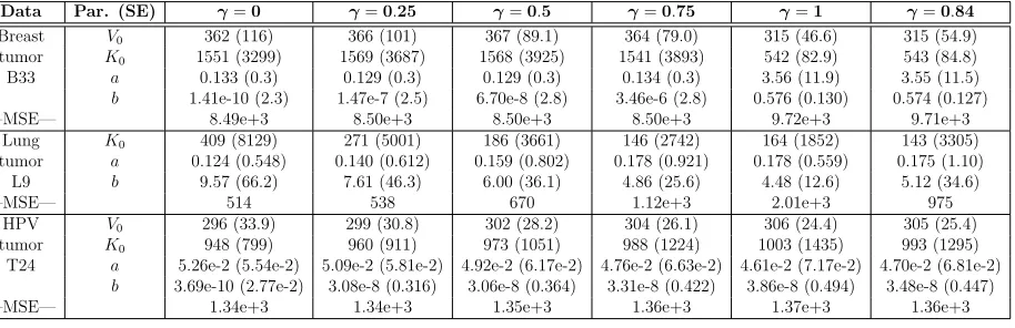
4.2.4 Dynamic carrying capacity

For the breast and lung tumor data, parameter estimates vary for a with >10% difference. The SEs for the estimates of a, however, are>100% of the estimate for the most part. The MSEs for the breast tumor data do not vary much (<6.5% difference), indicating that the model fit is not sensitive to a. The estimates forK0 and bvary for B16 and B33, but not for

the other breast tumors. The SEs for these estimates for B16 are much larger forγ = 0,0.25 than the otherγ’s. For B33, the SEs for these estimates are much larger forγ = 0.84,1 than the other γ’s.

The MSEs for the lung tumor data vary quite a bit (18−52% difference), with the MSEs for γ = 0,0.25 consistently the smallest. The estimates for K0 also vary a lot (17.5−70%)

(22)

There are no consistent results amongst the HPV tumor data sets besides the percentage difference for MSEs being < 4%. Some of the parameter estimates vary for T4 and T9, however the SEs for these estimates are all >40% the estimate.

Breast V0 362 (116) 366 (101) 367 (89.1) 364 (79.0) 315 (46.6) 315 (54.9)

tumor K0 1551 (3299) 1569 (3687) 1568 (3925) 1541 (3893) 542 (82.9) 543 (84.8)

B33 a 0.133 (0.3) 0.129 (0.3) 0.129 (0.3) 0.134 (0.3) 3.56 (11.9) 3.55 (11.5)

b 1.41e-10 (2.3) 1.47e-7 (2.5) 6.70e-8 (2.8) 3.46e-6 (2.8) 0.576 (0.130) 0.574 (0.127)

—MSE— 8.49e+3 8.50e+3 8.50e+3 8.50e+3 9.72e+3 9.71e+3

Lung K0 409 (8129) 271 (5001) 186 (3661) 146 (2742) 164 (1852) 143 (3305)

tumor a 0.124 (0.548) 0.140 (0.612) 0.159 (0.802) 0.178 (0.921) 0.178 (0.559) 0.175 (1.10)

L9 b 9.57 (66.2) 7.61 (46.3) 6.00 (36.1) 4.86 (25.6) 4.48 (12.6) 5.12 (34.6)

—MSE— 514 538 670 1.12e+3 2.01e+3 975

HPV V0 296 (33.9) 299 (30.8) 302 (28.2) 304 (26.1) 306 (24.4) 305 (25.4)

tumor K0 948 (799) 960 (911) 973 (1051) 988 (1224) 1003 (1435) 993 (1295)

T24 a 5.26e-2 (5.54e-2) 5.09e-2 (5.81e-2) 4.92e-2 (6.17e-2) 4.76e-2 (6.63e-2) 4.61e-2 (7.17e-2) 4.70e-2 (6.81e-2)

b 3.69e-10 (2.77e-2) 3.08e-8 (0.316) 3.06e-8 (0.364) 3.31e-8 (0.422) 3.86e-8 (0.494) 3.48e-8 (0.447)

—MSE— 1.34e+3 1.34e+3 1.35e+3 1.36e+3 1.37e+3 1.36e+3

Table 4: Parameter estimates, SEs, and MSEs using the dynamic carrying capacity model.

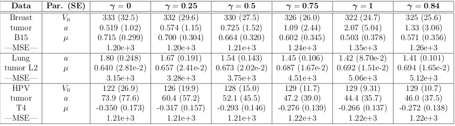
4.2.5 Power law

For the breast tumor data, the estimates for a and µ have >10% difference with SEs that are > 40% of the estimate. While the MSEs do vary for B16 and B31 (with 7.93−9.46% difference), the MSEs are consistent for B15 and B33 with<4% difference. Overall, however, the MSE for γ = 0 is consistently the smallest and the MSE for γ = 1 the largest.

For the lung tumor data, the estimates for a vary with 8−12% difference. In this case, we actually see SEs < 16% of the estimate. Further, we see 18−60% difference in MSEs, with the smallest MSE whenγ = 0 and the largest MSE whenγ = 1 except for L2 for which

γ = 0.84 gives the largest MSE. These results indicate that, if the power law model is a reasonable mathematical model for lung tumor growth, then the error appears to follow an absolute error statistical model (γ = 0).

For the HPV tumor data, the estimates for a vary with γ. However, the SEs are>80% of the estimates and the difference in MSEs is < 2% indicating that the model fits are not sensitive to a.

An observation from the breast tumor results that may or may not be significant is that the estimates for µ are all positive except for B31 when γ = 0.84,1 and for B33 for all γ

(23)

Breast V0 333 (32.5) 332 (29.6) 330 (27.5) 326 (26.0) 322 (24.7) 325 (25.6)

tumor a 0.519 (1.02) 0.574 (1.15) 0.725 (1.52) 1.09 (2.44) 2.07 (5.04) 1.33 (3.06)

B15 µ 0.715 (0.299) 0.700 (0.304) 0.664 (0.320) 0.602 (0.345) 0.503 (0.378) 0.571 (0.356)

—MSE— 1.20e+3 1.20e+3 1.21e+3 1.24e+3 1.35e+3 1.26e+3

Lung a 1.80 (0.248) 1.67 (0.191) 1.54 (0.143) 1.45 (0.106) 1.42 (8.70e-2) 1.41 (0.101)

tumor L2 µ 0.640 (2.81e-2) 0.657 (2.41e-2) 0.673 (2.02e-2) 0.687 (1.67e-2) 0.692 (1.51e-2) 0.694 (1.65e-2)

—MSE— 3.15e+3 3.28e+3 3.75e+3 4.51e+3 5.06e+3 5.12e+3

HPV V0 122 (26.9) 126 (19.9) 128 (15.0) 129 (11.7) 129 (9.31) 129 (10.7)

tumor a 73.9 (77.6) 60.4 (57.2) 52.1 (45.5) 47.2 (39.0) 44.4 (35.7) 46.0 (37.5)

T4 µ -0.350 (0.173) -0.317 (0.157) -0.293 (0.146) -0.276 (0.139) -0.266 (0.137) -0.272 (0.138)

—MSE— 1.21e+3 1.21e+3 1.21e+3 1.22e+3 1.22e+3 1.22e+3

Table 5: Parameter estimates, SEs, and MSEs using the power law model.

4.2.6 Von Bertalanffy

For most of the breast and HPV tumors, the estimates fora, b, andµvary a great deal with

> 30% difference for the breast tumor data and > 21% difference for the HPV data. The exceptions to this are breast tumor B15, for which the difference in estimates forb is 0.04%, HPV tumor T9, for which the difference in estimates for a and µ are <5.5%, and T24, for which the difference in estimates for a, b, and µ are < 4%. Regardless of whether or not the estimates for a and b vary, however, the SEs are consistently >100%. The difference in MSEs for the breast tumor data is<4.5% with the exception of B16 for which the difference in MSE is 7.92%. For the HPV tumor data, the difference in MSEs are <3%.

For the lung tumor data, the difference in estimates for b are >62% with SEs that are

>100% of the estimates. The rest of the results for the lung tumor data are not consistent across the lung tumors except that the difference in MSEs are >25%. When γ = 1, we see the MSEs are much larger than for the rest of the γ’s, and the smallest MSE occurs when

γ = 0.

Breast V0 327 (71.9) 323 (62.2) 314 (54.0) 305 (45.3) 296 (36.8) 302 (42.2)

tumor a 0.227 (1.37) 3.06 (1.12e+4) 0.742 (32.8) 1.89 (68.1) 6.27 (169) 2.84 (92.3)

B16 b 1.00e-4 (17.5) 2.86 (1.12e+4) 1.63e-4 (3.37) 1.00e-4 (1.54) 1.02e-4 (0.752) 1.00e-4 (1.17)

µ 0.852 (30.4) 0.994 (22.3) 0.672 (12.7) 0.528 (8.25) 0.343 (5.50) 0.465 (7.08)

—MSE— 3.34e+3 3.36e+3 3.45e+3 3.71e+3 4.31e+3 3.88e+3

Lung a 0.705 (0.205) 0.722 (0.202) 0.759 (0.178) 0.857 (0.122) 1.02 (0.173) 0.729 (0.279)

tumor b 1.67e-9 (0.529) 3.52e-4 (0.518) 2.96e-9 (0.503) 2.02e-9 (0.420) 6.75e-7 (0.332) 2.47e-6 (0.627)

L4 µ 0.807 (0.363) 0.801 (0.359) 0.789 (0.364) 0.759 (0.341) 0.713 (0.312) 0.798 (0.424)

—MSE— 1.42e+3 1.43e+3 1.55e+3 2.59e+3 7.45e+3 1.48e+3

HPV V0 254 (41.4) 255 (35.5) 256 (30.5) 257 (26.2) 258 (22.6) 257 (24.9)

tumor a 1.18 (3.74) 1.19 (7.20) 1.25 (15.5) 1.32 (23.0) 1.38 (29.8) 1.34 (25.5)

T9 b 0.363 (8.10) 0.522 (15.8) 0.650 (22.8) 0.746 (29.4) 0.836 (35.5) 0.779 (31.6)

µ 0.812 (4.05) 0.869 (3.86) 0.894 (3.67) 0.910 (3.49) 0.920 (3.33) 0.914 (3.43) —MSE—

1.86e+3 1.86e+3 1.86e+3 1.86e+3 1.86e+3 1.86e+3

(24)

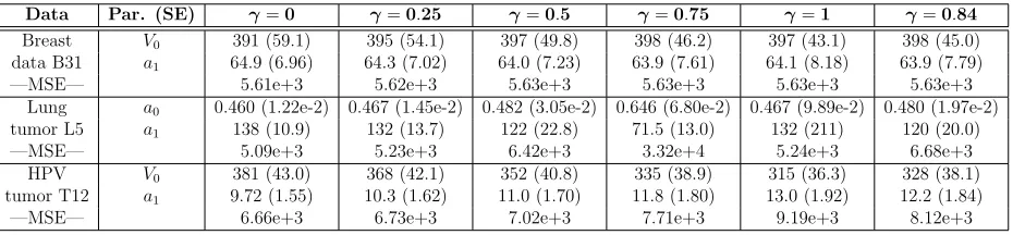
4.2.7 Exponential linear

For the breast tumor data, the statistical error model does not appear to affect the results and the difference in parameter estimates and MSEs are ≤4.5%.

For the lung tumor data, the difference in parameters estimates are 9.74−26.8% with the exception of L4 for which the difference in estimates are 2.24−6.84%. For the most part, the smallest SEs (relative to the estimate) occur when γ = 0 and the largest occur when

γ = 1. The difference in MSEs are ≥20%, with the smallest occurring when γ = 0 and the largest when γ = 0.75 or γ = 1.

For the HPV tumor data, the parameter estimates do not vary much except for tumor T12 for which the difference in estimates for a1 is 9%. We do not see any difference in SEs

acrossγvalues, which are approximately between 15 and 16% of the estimate. The difference in MSEs for T12 is 10.1% with the smallest MSE occurring whenγ = 0 and the largest when

γ = 1. The difference in MSE for the rest of the HPV tumors are<4%.

Breast V0 391 (59.1) 395 (54.1) 397 (49.8) 398 (46.2) 397 (43.1) 398 (45.0)

data B31 a1 64.9 (6.96) 64.3 (7.02) 64.0 (7.23) 63.9 (7.61) 64.1 (8.18) 63.9 (7.79)

—MSE— 5.61e+3 5.62e+3 5.63e+3 5.63e+3 5.63e+3 5.63e+3

Lung a0 0.460 (1.22e-2) 0.467 (1.45e-2) 0.482 (3.05e-2) 0.646 (6.80e-2) 0.467 (9.89e-2) 0.480 (1.97e-2)

tumor L5 a1 138 (10.9) 132 (13.7) 122 (22.8) 71.5 (13.0) 132 (211) 120 (20.0)

—MSE— 5.09e+3 5.23e+3 6.42e+3 3.32e+4 5.24e+3 6.68e+3

HPV V0 381 (43.0) 368 (42.1) 352 (40.8) 335 (38.9) 315 (36.3) 328 (38.1)

tumor T12 a1 9.72 (1.55) 10.3 (1.62) 11.0 (1.70) 11.8 (1.80) 13.0 (1.92) 12.2 (1.84)

—MSE— 6.66e+3 6.73e+3 7.02e+3 7.71e+3 9.19e+3 8.12e+3

Table 7: Parameter estimates, SEs, and MSEs using the exponential linear model.

4.3 Results summary: Effects of statistical models on the

mathe-matical model fits

Following the above observations, we discuss the overall effects of statistical models on the mathematical model fits, parameter estimates, standard errors, and mean squared errors for the seven mathematical models considered.

4.3.1 Logistic

(25)

4.3.2 Gompertz

The Gompertz model provides a reasonable visual model fit regardless of γ values for each data set. For the lung data, as γ increases, the MSEs increase, but the parameter estimates and SEs were consistent across statistical models. The breast data showed variance in the a

and β parameters, where each of these had standard errors on the same order of magnitude or larger. This suggests that there is not enough data to estimate these parameters. MSEs were consistent for the breast data, suggesting that when coupled with large standard errors, the model fit is not sensitive to a orβ. The Gompertz model fares well in all four criterion for the HPV data. Benzekry et al. concluded Gompertz provided the best model fit for both the lung and breast tumors. In the HPV tumor study the authors chose to exclusively use Gompertz due to the models capability to decrease the growth rate as the tumor increases in size, [13]. We note that the Gompertz model did not rank as best in any of our findings given in the AICc rankings below.

4.3.3 Generalized logistic

All three data sets give reasonable visual fits across all γ values when using the generalized logistic model. We see that the a and ν parameters have standard errors of at least one order of magnitude larger than the parameter estimate for all three data sets. Additionally, the breast and lung tumor data sets have large SEs for K. This implies that there is not enough information in the data to properly estimate these parameters. Except for the lung tumors, the MSEs are consistent acrossγ values, meaning that the model is not sensitive to those parameters with large standard errors in each of the data sets.

4.3.4 Dynamic carrying capacity

In this model, we see that the HPV and lung tumor data sets have reasonable visual fits. However, we observe overfitting in the plots for the breast data set. The parameter estimates and standard errors for V0 in the HPV data set were consistent and on a lesser order of

magnitude than the estimates, respectively. The MSEs for the HPV data set were consistent as well. All other parameters in all other data sets, across all γ, varied largely and showed great uncertainty in terms of SEs. This suggests that the data does not contain enough information to estimate the parameters, and further, that this is not an appropriate model for these data sets.

4.3.5 Power law

The visual model fits for this model are reasonable when applied to the lung and HPV data sets. For the breast data, as γ increases, we see a flattening of the curvature of the fit. In some cases, the concavity flips after a certain γ value. The parameter estimates for a and

(26)

as a secondary model to fit the lung tumor data. Our findings support those of Benzekry et al., for breast (although the estimated values for µvaried in sign) as well as lung tumors but were not particularly useful for the HPV data from [13].

4.3.6 Von Bertalanffy

The visual model fits for the lung and HPV data are consistent and reasonable for allγ. The breast data plots show a flattening of the fit curve through the data points asγincreases. The

a and b parameter estimates vary greatly across γ values for the breast data. The standard errors for these parameters are often a couple orders of magnitude larger than the estimates for all data sets investigated here. The standard errors for µ are larger in magnitude than the parameter estimates for the breast and HPV data sets as well. Aside from lung data when γ = 1, the MSEs are fairly consistent suggesting that the models are not sensitive to these parameters.

4.3.7 Exponential linear

The exponential linear model provides a reasonable visual model fit for the breast tumor data. In the HPV data set, we see that this model is not appropriate for two of the tumors, as the data does not follow a linear behavior. Note that the breast and HPV data sets have exclusively linear plots because of the formulation of the model (see 2.1.7 and the note before Section 4.1). For the lung data set, we see both exponential and linear sections of growth. In the lung tumor plots, when γ ≥ 0.75 the model fit underestimates the volume of the tumor, as it shifts to a linear growth rate too soon. We see that across all γ values, all of the parameter estimates, standard errors, and mean squared errors are consistent and reasonable, except for γ = 1 in the lung data set. In this case, the standard error fora1 was

larger than the parameter estimate; we note that non-convergence of the minimizer was an issue here.

4.4 Model Comparison

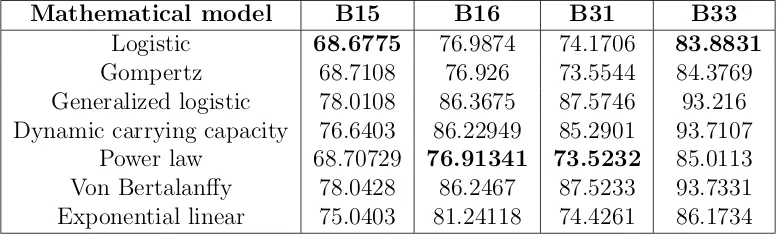
Based on our observations, the choice of statistical error model does not have a predictible or meaningful effect on model fit, parameter estimates, or SEs for data with a small sample size. We see that almost all of the data sets and mathematical models considered in this study revealed γ ≤ 0.25 corresponded to a reasonable choice of statistical error model. Thus, we suggest that for tumor growth data with small sample size, using simpler statistical models like the absolute error model is sufficient. With this assumption, we compared seven mathematical models to select the ones that most accurately fit each of the three tumor data sets. We use a small sample Akaike information criterion AICc and let ˆθ be the ordinary

(27)

Mathematical model B15 B16 B31 B33

Logistic 68.6775 76.9874 74.1706 83.8831

Gompertz 68.7108 76.926 73.5544 84.3769 Generalized logistic 78.0108 86.3675 87.5746 93.216 Dynamic carrying capacity 76.6403 86.22949 85.2901 93.7107

Power law 68.70729 76.91341 73.5232 85.0113 Von Bertalanffy 78.0428 86.2467 87.5233 93.7331 Exponential linear 75.0403 81.24118 74.4261 86.1734

Table 8: AICc scores for four breast tumor data using absolute error statistical model

Mathematical model L2 L4 L5 L9

Logistic 89.9735 105.5746 101.1007 84.9384 Gompertz 87.1341 93.8046 92.3032 71.8832 Generalized logistic 85.6942 97.5030 96.2457 76.2243 Dynamic carrying capacity 91.0634 95.7695 95.6755 72.4129 Power law 94.0932 92.4395 91.8300 69.4471

Von Bertalanffy 91.4186 96.1062 95.7513 73.7327 Exponential linear 87.3220 106.8956 99.3937 87.6840

Table 9: AICc scores for four lung tumor data using absolute error statistical model

Mathematical model T4 T9 T12 T24

Logistic 167.5015 187.84 112.5700 101.5624

Gompertz 167.6620 187.899 111.1681 102.24 Generalized logistic 170.389 190.749 115.21 105.5 Dynamic carrying capacity 170.621 189.065 109.10 106.57

Power law 170.457 195.415 113.02 104.2237 Von Bertalanffy 170.6813 190.814 113.82 106.59 Exponential linear 174.701 201.077 131.65 108.31

Table 10: AICc scores for four HPV tumor data using absolute error statistical model

Based on the AICc scores given in Tables 8-10, the logistic, power law, and Gompertz

models give the best fits for the breast tumor data. For the lung tumor data, the power law, Gompertz, and dynamic carrying capacity are the top three mathematical models that provide the best fits to the data. And finally, for the HPV tumor data, in general the logistic and Gompertz models give the best fits to the data.

5 Discussion and Conclusions

(28)

(breast, lung and skin) of tumor data sets. We thoroughly examined the performance of the mathematical models and the effects of the choice of the statistical models (γ values) using four criteria. Theγvalues we used range from 0 to 1. To determine the appropriate statistical error models, we analyzed the consistency of parameter estimates, standard errors (SEs) and mean squared errors (MSEs). In our study, we discovered that if a data set is small, simple residual plots cannot effectively provide information to determine if a statistical error model is appropriate. Neither can second order differencing-based techniques be used to choose the appropriate statistical error model. Both of these methods require the ability to see a pattern or to determine there is no pattern. The small sample size makes any assertions on patterns or randomness unreliable at best since the addition or removal of a single data point can often make one come to an opposite conclusion than originally determined. Therefore, we have to examine the impact of the choice of statistical error model on the overall model fit (parameter estimates, SEs, MSEs, AICc) instead to determine the best choice for statistical error model.

In general, we observed that whenγ is large (oftenγ ≥0.75) visual model fits begin to look inaccurate; similarly, SEs and MSEs tend to increase to unreasonable sizes. Therefore, for small sample sizes, a simpler statistical error model like absolute error is sufficient as the model fits either deteriorated or did not improve when using other statistical models (γ >0) due to the sparsity in the data. Assuming that absolute error is the appropriate statistical error model, we used likelihood based model selection criterion (AICc) to determine the

mathematical models that best fit each of the three types of tumor data. According to our findings, logistic, power law and Gompertz models produce the best fit for the breast tumor data; power law, Gompertz and dynamic carrying capacity are suited for the lung tumor data; and, logistic and Gompertz models provide the best fits for the skin (HPV) tumor data. Based on our proposed evaluation criteria, we found that the Gompertz model fit the HPV data best (despite not featuring as a selection based on AICc), the power law model

fit the lung tumor data best, and there was not a best model that consistently fit the breast tumor data set based on our criteria due to the small sample size.

In general, to estimate mathematical model parameters, the amount of data and informa-tion content in the data are crucial. Using the breast and lung tumor data sets, we observed that one can only estimate at most two parameters with a reasonable accuracy. In the case of skin (HPV) tumor data sets, one can estimate up to three parameters due to the relatively large sample size of the data. The lack of information in the data increases the uncertainty in parameter estimation. For example, we observed for models that have many parameters, SEs were very large. In some cases, for models like the logistic model, the parameter esti-mates for carrying capacity K were also very inconsistent and the standard errors were very large. Even though some parameters were fixed (for example initial condition V0, in lung

(29)

perform better for these short time interval data sets as only the linear part is fitted and the data contains the information to estimate the few parameters in the linear model.

Based on the above observations, we believe future research is necessary to determine the minimum amount of data needed to accurately estimate parameters in a mathematical model and for the statistical error model to affect the model fits. Specifically, further investigation is desirable on the experimental design in regards to measurement frequency and time span of the tumor measurements. In addition, more research is necessary to explore the minimum number of observations required for methods like residual plots to provide useful information regarding the appropriate statistical error model and for the second order differencing based technique to be valid. Both of the articles we used to gather the data sets were limited by their time scales and frequency of measurements, which limited the accuracy of model parameter estimation [8, 13].

Acknowledgment

This research was supported in part by the National Institute on Alcohol Abuse and Al-coholism under grant number 1R01AA022714-01A1, and in part by the Air Force Office of Scientific Research under grant number AFOSR FA9550-15-1-0298.

References

[1] H.T. Banks, K. Bekele-Maxwell, L. Bociu, M. Noorman and K. Tillman, The complex-step method for sensitivity analysis of non-smooth problems arising in biology, Eurasian

Journal of Mathematical and Computer Applications, 3 (2015), 15–68.

[2] H.T. Banks, K. Bekele-Maxwell, L. Bociu, and C. Wang, Sensitivity via the complex-step method for delay differential equations with non-smooth initial data, CRSC-TR16-09, Center for Research in Scientific Computation, N. C. State Univer-sity, Raleigh, NC, July, 2016, Quarterly of Applied Mathematics, November 2, 2016. http://dx.doi.org/10.1090/qam/1458.

[3] H. T. Banks, J. Catenacci, and S. Hu, Use of difference-based methods to explore statistical and mathematical model discrepancy in inverse problems,Journal of Inverse and Ill-posed Problems, 24 (2016), 413–433.

[4] H.T. Banks, S. Hu, and W.C. Thompson, Modeling and Inverse Problems in the

Pres-ence of Uncertainty, Chapman & Hall/CRC Press, Boca Raton, FL, 2014.

[5] H.T. Banks and Michele L. Joyner, AIC under the framework of least squares estimation, CRSC-TR17-09, Center for Research in Scientific Computation, N. C. State University, Raleigh, NC, May, 2017; Applied Math Letters, to appear.

(30)

in Scientific Computation, N. C. State University, Raleigh, NC, June, 2017; J. Inverse

and Ill-Posed Problems, submitted.

[7] H. T. Banks and H. T. Tran,Mathematical and Experimental Modeling of Physical and

Biological Processes, CRC Press, Boca Raton, FL, 2009.

[8] S. Benzekry, C. Lamont, B. Afshin, A. Tracz, JML Ebos, et al. , Classical mathematical models for description and prediction of experimental tumor growth. PLoS Comput

Biol. 10(8) (2014): e1003800. doi:10.1371/journal.pcbi.1003800

[9] K.P. Burnham and D.R. Anderson, Information and Likelihood Theory: A Practical

Information-Theoretic Approach, Springer-Verlag, New York, 2002.

[10] M. Davidian and D.M. Giltinan, Nonlinear Models for Repeated Measurement Data, Chapman and Hall, London, 2000.

[11] A. Ronald Gallant,Nonlinear Statistical Models, John Wiley and Sons, New York, 1987.

[12] D. Hart, E.Shochat, and Z. Agur, The growth law of primary breast cancer as inferred from mammography screening trials data.British Journal of Cancer, 78(3), (1998) 382.

[13] C. Loizides, D. Lacovides, M.M. Hadjiandreou, G. Rizki, A. Achilleos, K. Strati, et al. Model-based tumor growth dynamics and therapy response in a mouse model of de novo carcinogenesis. PLoS ONE, 10(12) (2015): e0143840.http://doi.orgg/10.1371/journal.pone.0143840

[14] J. N. Lyness, Numerical algorithms based on the theory of complex variables, Proc.

ACM 22nd Nat. Conf., 4 (1967), 124—134.

[15] J. N. Lyness and C. B. Moler, Numerical differation of analytic functions, SIAM J.

Numer. Anal., 4(1967), 202—210.

[16] Joaquim R. R. A. Martins, Ilan M. Kroo, and Juan J. Alonso, An automated method for sensitivity analysis using complex variables. AIAA Paper 2000-0689 (Jan.), 2000.

[17] Joaquim R. R. A. Martins, Peter Sturdza, and Juan J. Alonso. The complex-step deriva-tive approximation. Journal ACM Transactions on Mathematical Software (TOMS), 2003.

[18] H. Murphy, H. Jaafari, and H.M. Dobrovolny, Differences in predictions of ODE models of tumor growth: a cautionary example. BMC Cancer, 16(1) (2016), 163.

[19] A. Rohatgi, [WebPlotDigitizer], (2017), Retrieved from http://arohatgi.info/WebPlotDigitizer

(31)

[21] G.A.F. Seber and C.J. Wild, Nonlinear Regression, J. Wiley & Sons, Hoboken, NJ, 2003.

[22] J.A. Spratt, D. Von Fournier, J.S. Spratt, and E.E. Weber, Decelerating growth and human breast cancer, Cancer, 71(6) (1993), 2013-2019.

[23] B. Tummers, [DataThief III], (2006), Retrieved from http://datathief.org/

[24] Y. Tanaka, K. Hongo, T. Tada, K. Sakai, Y. Kakizawa, and S. Kobayashi, Growth pattern and rate in residual nonfunctioning pituitary adenomas: correlations among tumor volume doubling time, patient age, and MIB-1 index. Journal of Neurosurgery,

98(2) (2003), 359-365.