Substitution Rates Under Stabilizing Selection

(1)

Copyright 0 1987 by the Genetics Society of America

Substitution Rates Under Stabilizing Selection

Alan Hastings

Department of Mathematics and Division of Environmental Studies, University of Calijornia, Davis, Calijornia 956 16 Manuscript received December 3, 1986

Revised copy accepted March 27, 1987

ABSTRACT

Allelic substitutions under stabilizing phenotypic selection on quantitative traits are studied in Monte Carlo simulations of 8 and 16 loci. The results are compared and contrasted to analytical

models based on work of M. Kimura for two and “infinite” loci. Selection strengths of S = 4Nd approximately four (which correspond to reasonable strengths of selection for quantitative characters)

can retard substitution rates tenfold relative to rates under neutrality. An important finding is a

strong dependence of per locus substitution rates on the number of loci.

N E of the most interesting and important ques-

0

tions facing population genetics today is the relationship between selection at the level of the organism and selection at the level of the locus. At the level of the organism, or quantitative trait, selection is strong and ubiquitous (ENDLER 1986). At the level of the locus the importance of selection and of random forces in determining the dynamics of allele frequencies has been the subject of intense debate (KIMURA

1983). What is the connection between these two levels? Two primary questions emerge. First, is evolution at loci determining quantitative traits different from evolution at neutral loci? If the answer to this question is affirmative, can these differences be studied at the level of the single locus or are multilocus models needed?

This question also relates tangentially to part of WRIGHT’S (1 978) shifting balance theory of evolution. WRIGHT was concerned with the probability of shifting from one peak to another, which in a model with constant fitnesses, stabilizing selection and equivalent loci corresponds to substitutions at two loci which lead to no change in the phenotype. WRIGHT discussed order of magnitude estimates of the speed of this process based on two locus ideas.

T h e relationship between selection at the level of a quantitative trait and the single locus level has been examined by a number of authors, in particular KI- MURA and CROW (1978), BULMER (1971-1974, 1976, 1980), KIMURA (1981, 1985) and NAGYLAKI (1984). There are two problems that these authors have fo- cused on. One has been the determination of selective values at individual loci. KIMURA and CROW (1978) treated this question, which does not involve dynamics. T h e results are phrased in the following fashion. If the level of genetic variability is held constant, the per locus selection values must go down as the number of loci is increased. Note however, that if the level of

Genetics 1 1 6 479-486 (July, 1987)

variability is not determined a priori, but from values for the strength of selection and mutation, the afore- mentioned conclusion does not hold.

Of more interest here are the analyses proposed by

KIMURA (1 98 1, 1985), who considered a second problem: dynamics of alleles at loci which determine a character undergoing stabilizing selection under two quite different assumptions. In one case, he used what I will call an “infinite locus” approximation and in the other case he studied an explicit two locus model.

For the “infinite locus” approximation, KIMURA ( 1 98 1) used a diffusion analysis to determine the rates of substitution of alleles at these loci. This analysis concentrated on a single locus at a time, dealing with other loci as “background.” KIMURA’S analysis shows that the rate of substitution under this model is much larger than the substitution rate for deleterious loci, for similar selective values. This analysis also predicts that selection always retards the rate of substitution relative to a neutral locus.

In studying a two-locus model, KIMURA (1985) used a different analysis, numerically solving a diffusion equation model for a system with one-way mutation, which led to different predictions. T h e quantity of interest was the mean time for substitution at two loci with a haploid selection scheme whereby single mutants were selected against but double mutants had the same fitness as the initial type. In this model and analysis, weak selection actually accelerated the substitution rate. Also, as I discuss below, the answers given by the two-locus model and analysis and the “infinite locus” model differ for stronger selection, where the “infinite locus” model predicts faster substitution rates than the two-locus model.

(2)

studies of the numerical solution of the two-locus model, extending the results to a diploid selection scheme and also to a larger range of parameters. On the other hand, I will describe extensive simulations with 8 and 16 loci which help detail the ranges of applicability of the two approximations used by KI-

MURA, and reveal a strong dependence of per locus substitution rates on the number of loci when selection is strong.

GENERAL MODEL

T h e general model describing the relationship between a quantitative character and underlying loci can be traced back to FISHER (1918). T h e model here is more restricted and assumes that a character is determined additively by a large number of loci plus some environmental effects, so that if P is the phenotype

P = G + E , (1)

G = ai

+

a(

(2)

where

i

where ai is the effect of one allele at locus

i

and a: is the effect of the other allele and the sum is over all loci

i

which determine the character.

T h e relationship between selection at the level of a single locus and at the level of a quantitative trait has been most extensively studied in the case of Gaussian stabilizing selection (KIMURA and C R O W 1978, CROW and KIMURA 1978, BULMER 1980, KIMURA 1981;

NAGYLAKI 1984). Here, without loss of generality, let the optimum phenotype be 0 on some scale. Take the fitness W ( X ) of an individual with phenotype x to be

W ( X ) = exp(-kx2), (3)

where

k

is a measure of the strength of selection. For small values of

K,

the fitness is very well approximated by:

w ( x )

=

1 - Kx2, _{( 3 4}

and this approximation is used at times below to simplify algebra. A further assumption made is that the phenotype under consideration is determined by a large number of loci, each with small effect. Then, the following equations describing changes due to selection have been derived by BULMER (1980) and

KIMURA (1 98 l), and shown to hold under more general conditions by NAGYLAKI (1 984). Let p represent the frequency of the allele Az. Let the phenotypic contribution of an A2A2 individual be a , that of an

A2A1 individual be 0, and that of an A l A l individual be -a. Then, the selective advantage of A2 over A1 is

s = -mXa

+

(A2 m2

-

~ ) ( 1 / 2

-

p ) a 2 , (4)

where

A = 2k/(l

+

K )

_{( 5 )}

and m is the mean value of the character in question in the population. Thus the change in one generation d u e to selection at this locus is given by:

sp

= sp(1

-

p ) .

(6)

T h e haploid form of selection implied by (6) arises from the additivity assumption and an assumption of weak selection.

Infinite locus approximation: KIMURA (1 98 1) used Equations 4-6 to form the basis of a study of the behavior of mutant alleles in a finite population under stabilizing selection. T h e question dealt with by KI- MURA that is of primary interest here is the probability of fixation of a mutant allele. Denote the effective population size by Ne. Following KIMURA (1 98 1) let

PI

= -Xma

( 7 )

(8)

(9)

and

P2

= X(1

-

Xm2)a2/2,

s =

PI

-

PZ(1

-

2 p ) .

so (4) becomes:

Substituting (9) into (6) shows that both fixation states are stable with an unstable polymorphic equilibrium. Thus, as noted by KIMURA, each locus appears underdominant. KIMURA then shows that the probability of fixation, U , of a new mutant is given by

exp(-Blx

+

B2x(l

-

x ) ) d x ] , (10)

where

and

This fixation probability should be contrasted to that of a neutral mutant, which is 1/2N [to which (10) reduces when there is no selection].

(3)

Substitutions Under Selection 48 1

TABLE 1

Two-locus fitness scheme embodying stabilizing selection

BB Bb bb

AA 1 1 - k 1

-

4 k

Aa 1 - k 1 1 - k

aa 1 - 4 k 1 - k 1

The parameter k measures the strength of selection. Here it is assumed small so the approximation (3a) to Gaussian selection is used.

pear underdominant. Part of the goal of the current paper is to examine when the approximation used by

KIMURA is a good one.

KIMURA then goes further by taking m to be 0, and evaluating (10) numerically to produce a table of the relative probability of fixation of a new mutant under stabilizing selection to that obtained for a neutral allele. The probability from (1 0) is then compared to that of an unconditionally deleterious allele. Following this approach, values of the relative time for substitutions under this approximation will be compared below to results from simulations. As KIMURA (1981) notes, this analysis predicts that extensive substitutions are still possible under stabilizing selection even when

S = ~ N J is as large as 8, where the rate of substitution is still 23% of the neutral rate.

Another way of viewing the approximation used by

KIMURA is that he assumes that as the allele frequencies change at some given locus, the allele frequencies change at all the other loci in such a way that the overall mean phenotype remains constant. This is the reason that selection at each locus appears underdominant. Another extreme possibility would be to assume that the allele frequencies at other loci remain un- changed as the allele frequencies at a given locus change-the phenotype is totally correlated with the particular locus under consideration. It appears quite clear that this should give a lower bound as to the rate of substitutions, while KIMURA’S approximation should give an upper bound. It is only if NJ is large enough that these two estimates will differ to a great enough extent that the predictions can be told apart, since for small

NJ

all substitutions would appear nearly neutral.

Two-locus approximation: Another approach to studying substitution under stabilizing selection was also introduced by KIMURA (1 985), who concentrated on studying substitution rates in a 2-locus model with one way recurrent mutation. Here a model with two

loci A and B is studied. Assume that the population is initially fixed for the alleles a and 6 at these two loci, and that a mutates to A and 6 to B at a rate Y per allele per generation. Let the effective population size be

Ne. Let T ( p , q ) be the average time until both A and B are fixed, given that the initial frequencies of A and

B are

p

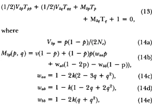
and q, respectively. KIMURA shows that T satisfies the following equation (where the subscripts on T denote partial derivatives):

( 1 3 ) ( /2)v6pTpp

+

(1/2)v&qTqq

+

M6pTp

+

M,T,

+

1 = 0, where

V6, = P(1

-

P)/(2Ne) (144

U4b)

w,, = 1 - 2 4 2

-

3q

+

q 2 ) , ( 1 4c)

wab 1

-

k(

1 - 2q

+

2q2), ( 1 4 4

W6b = 1

-

2 k ( q

+

q 2 ) , ( 1 4 4

M 6 p ( p 9 q ) = V ( l

-

p )

+

(1

-

p)p(waap

-b wad1

-

2p)

-

w b b ( l

-

p)),

with V, and M , defined similarly. Note that the mean changes in allele frequencies, Map(p, q ) and M , ( p , q),

depend on the mutation rate U . The boundary condi-

tions are:

l i m w T p ( p , q ) is finite lim, T,(p, q ) is finite

(154

(15b) and that along the other boundaries the appropriate one dimensional equation is satisfied, namely:

(1/2)VapTpp(P, 1) -I- Msp(p, l)Tp(p, 1)

+

1 = 0 , (16) which itself has boundary conditions

and

Tp(O, 1) is finite (174

T(1, 1) = 0. (17b)

There is also a similar boundary condition along the boundary

p

= 1. The solution of (1 6)-( 17) is known, as it can be obtained by integration. KIMURA (1985) used this solution and solved (1 3 ) numerically using a finite difference method and Gauss-Side1 iteration. He assumed a haploid fitness scheme, and considered only the case 0 = 4Nev = 2. Among the results he found was the fact that weak selection actually accelerated the rate of substitution, in contrast to the “infinite locus” approximation.

(4)

.A

i

+J

3

5

2

v1

P 150

100

50

0 .

P

I

B

I

0.0 0.5 1.0 1.5 2.0 2.5 3.0 3.5 4.0

S

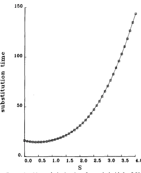
FIGURE 1.-Mean substitution times for two loci with B = 0.01.

The time units are 4 N e generations, with S = 4N&, with the fitness scheme in Table 1. The time T ( 0 , 0) to substitute at two loci is calculated from Equation 17.

100

0.

L

I

0.0 0.5 1.0 1.5 2.0 2.5 3.0 3.5 4.0

S

FIGURE 2.-Mean substitution times for two loci with 8 = 0.1.

The time units are 4 N , generations, with S = 4N&, with the fitness scheme in Table 1. The time T(0, 0) to substitute at two loci is calculated from Equation 17.

decreasing the time of joint fixation also occurs for the parameter values and selection schemes which I have chosen. Note in particular the contrast with the “infinite locus” approximation, where the substitution rate always is lower when there is selection than in the neutral case. Second, not surprisingly, the time to joint fixation depends strongly on both 8 and S, not simply the ratio of 8 to S. This can be seen by com- paring the two figures which give substitution times for different mutation rates. Third, keeping the ratio of 8 to S fixed, the time of joint fixation depends very strongly on population size, unlike the case of neutral mutations. (Compare the substitution times for 8 = 0.01 and S = 0.3 to the time for 8 = 0.1 and S = 3.0.) However, it is not clear how to translate the results of this analysis to ongoing substitution rates at a large number of loci controlling a single character. For the values of 8 chosen here, the substitution times at both loci for neutral alleles are almost exactly 3/2 the substitution time at a single locus, as would be the case if substitution times followed a Poisson distribution. In the neutral case and for sufficiently weak selection, substitution is a single locus phenomenon. By this I mean that substitution times at a particular locus are independent of substitution times at other loci. Hence, for weak selection, it would be incorrect to determine per locus substitution rates by taking the time to substitute at a pair of loci. However, for stronger selection, substitution is a two locus phenomenon and there is a large correlation between substitution times at different loci. This is because the mean of quantitative trait always remains close to the optimum with strong selection, so the only way a substitution can occur is for two loci to substitute at nearly the same time. Hence, for strong selection, the time to substitute a pair of loci might be relevant for determining single locus substitution rates. T h e fac- tors just described may actually be the reason for the decrease in substitution times with weak selection.

Simulation model: Simulations of a truly multilocus system should provide a guide to the dynamics of substitutions under stabilizing selection. Comparisons with the analyses of KIMURA just described should then allow an assessment of the assumptions made, and consequently provide further insight into the dynamics. I have thus used computer simulation to study the question of substitution under stabilizing selection. More complex analytic treatments appear very difficult, although the results of the computer simulations may provide a guide for future research.

(5)

Substitutions Under Selection 483

assumed to be on different chromosomes, or far enough apart on the same chromosome so that an assumption of free recombination is justified. Finally, mutation is assumed to be equally likely in both direc- tions. T h e effect of mutation on dynamics, when both alleles are at appreciable frequency, is likely to be insignificant, since the mutation rates used are small. I will now describe the computer simulation. More details are given in Appendix 11. I will begin by discussing the parameter values I used. T h e simulations were written in C and performed on IBM A T and compatible computers. I simulated a diploid population with 1024 individuals. I considered cases with both 8 and 16 loci. Note that estimates on the number of loci contributing to quantitative traits range from roughly ten to more than one hundred (FALCONER

198 1). Without loss of generality, I took the effect of each allele to be one. (This is the a parameter.) Until the other parameters are chosen, values of a merely represent a choice of scale. More precisely, at each locus there were two possible alleles, one which contributed 0 to the phenotypic score, and one which contributed 1. T h e optimum phenotype in each case corresponded to half 0 alleles and half 1 alleles-8 in the 8-locus case and 16 in the 16-locus case.

T h e choice of the other parameters requires more care. TURELLI (1984) has reviewed the literature on mutation rates and the strength of selection. I have chosen per locus mutation rates which are in line with estimates, but near the maximum estimates in order to obtain enough substitutions to form a reasonable study. Thus, the mutation rate per allele

per

generation was taken as either

9.77

X (approximately T h e strength of selection was also chosen to correspond to estimates reviewed in TURELLI (1 984), also providing values where KIMU- RA’s analysis suggests that alleles under stabilizing selection will behave differently than deleterious alleles. Thus

k

was taken as either 0.0001, 0.0005 or 0.001. This corresponds to values of S of 0.4096, 2.048 and 4.096.

T h e simulations just described may not provide an accurate representation of substitution rates if more than two alleles are segregating at a locus. Any mutation that occurs in the simulation when two alleles are segregating at a particular locus ends up not as a mutation to a new allele, but to an existing one. Thus the simulations may underestimate the rate of substitutions. For this reason, I have also simulated the neutral case, with S = K = 0.0. This provides a standard of comparison for substitution rates with selection.

T h e parameter values described above lead to a total of 16 different sets, when all possible combina- tions are used. For each set of parameters two different simulations were run (except for the cases with the strongest selection and 8 loci where four simula-

or 1.954 X

TABLE 2

Substitutions per locus as a function of R

Mutations per locus

k Loci e = 0.04 8 = 0.02

0.0 0.0 0.0001 0.0001 0.0005 0.0005 0.001 0.001

8 7.13 (2.45) 16 7.00 (2.58) 8 5.44 (3.20) 16 5.56 (2.17) 8 3.5 (1.93) 16 3.72 (2.02) 16 1.625 (1.18)

8 1

.oo

(1.02)

3.32 (2.00) 3.16 (1.68) 2.75 (1.53) 2.72 (1.59) 1.625 (1.31) 1.375 (1.07) 0.31 (0.54) 0.625 (0.87) The entries for 8- and 16-loci are the mean number and standard deviation (in parentheses) of substitutions per locus in 400,000 generations, as a result of two simulations, except for k = 0.001 and 8 loci, where four simulations were used. Here 0 = 4Nev, where

v is the mutation rate.

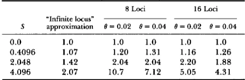
TABLE 3

Mean substitution times per locus for the simulations and the

“infinite locus” approximation, as compared to the neutral case

8 Loci 16 Loci

“Infinite locus”

S approximation 0 = 0.02 8 = 0.04 8 = 0.02 8 = 0.04

0.0 1

.o

1.0 1.0 1

.o

1

.o

0.4096 1.07 1.20 1.31 1.16 1.26 2.048 1.42 2.04 2.04 2.20 1.88 4.096 2.07 10.7 7.12 5.05 4.31

The figures in each column are mean substitution times divided by the mean time for S = 0.0. The times for the infinite locus approximation are from Equation 10. Here S = 4N,s and 0 = 4Nev, where v is the mutation rate. Since this is a multilocus phenotypic model, the S values at a given locus depend on the other loci; the value given above assumes zero mean for the phenotype.

tions were used), each lasting 400,000 generations. Note that under the parameters chosen, most loci are fixed for one allele most of the time, A substitution was recorded as occurring when a locus which was previously fixed for one allele became fixed for the other allele. (This was tested with the neutral case by using other less stringent fixation criteria such as counting a locus as fixed when the frequency of the common allele reached 0.99, which led to identical results.) Tests for fixation were done every 20 o r 40 generations, depending on the parameters. Moreover, the simulations were started with all loci fixed so the population was at the optimum. Studies of typical time courses also indicated that the above procedure was quite reasonable.

(6)

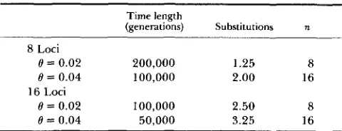
TABLE 4

Substitutions over time with R = 0.001

Time length

(generations) Substitutions n

8 Loci

0 = 0.02 200,000 1.25 8

8 = 0.04 100,000 2.00 16 0 = 0.02 100,000 2.50 8

0 = 0.04 50,000 3.25 16 16 Loci

The simulations are broken into blocks of 50,000-200,000 generations so an identical number of substitutions was expected in each block, and thus an ANOVA analysis could be performed (see Table 5) to determine causes of differences in substitution rates.

TABLE 5

Results of an ANOVA analysis of the substitutions with

R = 0.001

Source d.f. ss MS F,

Mutation rate 1 6.00 6.00 1.32 No. of loci 1 18.75 18.75 4.12* Interaction 1 0.00 0.00 0.00 Within 44 186.50 4.55

The analysis was performed by separating simulations into blocks of 50,000-200,000 generations (Table 4) so an identical number of substitutions was expected in each block. The one significant effect was the number of loci.

*

Significant at the 0.05 level.

for the simulations and the two analytical approximations. When interpreting Table 3, it is important to note that the mean times are for different aspects of substitution. Note that the infinite locus approximation always underestimates the retarding effect of selection on substitution rates, relative to the simulations. In all cases selection retards the rate of substitution, in agreement with the “infinite locus” model. For strong selection, the 2-locus model greatly over- estimates the retarding effect of selection on substitution relative to the simulations. This is to be expected, since the number of different pairs of loci increases as a quadratic function of the number of loci. Note however that the parameter value S = 0.4096 is one where the 2-locus model in fact says that the time until fixation of both mutants would be less than that for the neutral case, in contrast to the simulations.

T h e magnitude of the reduction in substitution rates is very striking, as given in Table 3. T h e reduction in substitution rates is much greater in the simulations than in the “infinite locus” model, although it is not quite as great as that of unconditionally deleterious alleles. This is most striking in the 8-locus case with the weakest mutation rates, where the strongest value of selection used, S = 4.096, leads to a ten-fold reduction in substitutions, relative to the neutral case. There is a strong dependence of the substitution rate on the number of loci for the strongest selection

value used (Tables 4 and 5), which may explain why the greatest reduction in substitution rates occurs for 8 loci and the weakest mutation rate. T o analyze this dependency the simulations were broken up into in- tervals which would have the same expected number of substitutions if the rate of substitutions depended linearly on the mutation rate and the number of loci. Given the fact that the time between substitutions was long relative to the time an allele was segregating, this introduces little bias. T h e resulting data was then analyzed using ANOVA techniques (SOKAL and ROHLF 198 1). This dependency of the substitution rates on the number of loci is not removed if a different scaling, say choosing parameters so that the total variance remains constant is used. In the weak selection cases, the per locus substitution rate appears to be independent of the number of loci, although the variance depends roughly linearly on the number of loci.

T h e reason why there is a strong dependency of the per locus mutation rate on the number of loci is apparent from an examination of the times of substitutions when S = 4.096. T h e substitutions basically occur in pairs, even when there are 16 loci. (This occurs because with strong selection, the population mean must always lie close to the optimum.) T h e results of a Kolmogorov-Smirnov test not surprisingly show that the mean times between substitutions differ significantly from a Poisson distribution, and additionally that the distribution of times for substitutions which bring the population from a “0” state to a “1” state are significantly larger than the times for substitutions which bring the population from a “1” state to a “0” state. Here a “0” state is one where if each locus were now fixed at the allele which most recently was fixed at that locus, the population mean for the trait would be at the optimum. Similarly, a “1” state would be one that was one allele (in either direction) away from the optimum.

(7)

Substitutions U n d e r Selection 485

DISCUSSION

I will now return to the two questions posed in the introduction regarding the dynamics of alleles under stabilizing selection. First, are these dynamics different from those of neutral alleles? From the simulations, some quantitative differences do emerge. For reasonable strengths of selection and reasonable mutation rates the substitution rates of alleles determining a phenotypic trait undergoing stabilizing selection can be an order of magnitude less than that of neutral alleles.

T h e second question posed in the introduction concerned the role of the number of loci in understanding allelic substitutions at loci determining a quantitative trait. There is one particularly intriguing feature of the analysis of substitution rates under stabilizing selection that does emerge here. These substitution rates may have a very strong dependence on the number of loci. This apparently is due to the fact that for strong stabilizing selection, substitution is essen- tially a 2-locus process. T h e number of different pairs of loci rises quadratically with the number of loci. This is one of the first examples of the (nonlinear) dependence on the number of loci of an evolutionarily important property in models of stabilizing selection. This suggests strongly that analyses of the models of quantitative genetics may have to take into account the number of loci. This may be particularly true for dynamic properties.

T h e possibility of determining the presence of stabilizing selection by examining single loci has not been answered by the results of the simulations here. In fact, the results here strongly suggest that differences in substitution rates of the order of magnitude ob- served here, or even larger, even though caused by stabilizing selection, could not be detected by obser- vations of substitutions at a single locus. Also note that substitution rates at one locus are affected by the number of other loci determining the trait under consideration.

One cautionary note is that the results reported here are for identical diallelic loci. It is not immedi- ately clear what the analogous results would be for other models. Work on this important question is currently in progress.

I thank ANGELA CHEER, JOHN GILLFSPIE, CHUCK LANGLEY and MIKE TURELLI for helpful discussions. I thank RUSS LANDE for comments on the paper. I thank the referees for a number of comments which improved both the presentation and the substance of the paper. Supported by United States Public Health Service grant R01 GM32130.

LITERATURE CITED

BULMER, M., 1971

BULMER, M., 1972

The effects of selection on genetic variability. The genetic variability of polygenic characters Am. Nat. 105: 201-2 1 1.

under optimizing selection, mutation and drift. Genet. Res. 1 9

T h e maintenance of the genetic variability of polygenic characters by heterozygous advantage. Genet. Res. BULMER, M., 1974 Linkage disequilibrium and genetic variability.

Genet. Res. 23: 281-289.

BULMER, M., 1976 T h e effect of selection on genetic variability: a simulation study. Genet. Res. 2 8 101-117.

BULMER, M., 1980 The Mathematical T h o r y of Quantitative Genetics.

Oxford University Press, New York.

ENDLER, J., 1986 Natural Selection in the Wild. Princeton Univer- sity Press, Princeton, N.J.

FALCONER, D., 198 1 Introduction to Quantitative Genetics, Second Edition. Longman, New York.

FISHER, R. A., 1918 The correlation between relatives on the supposition of Mendelian inheritance. Trans. R. Soc. Edinb. GILLESPIE, J., 1986 Natural selection and the molecular clock.

Mol. Biol. Evol. 3: 138-155.

KIMURA, M., 198 1 Possibility of extensive neutral evolution under stabilizing selection with special reference to non-random usage of synonymous codons. Proc. Natl. Acad. Sci. USA 7 8 5773- 5777.

The Neutral Theory of Molecular Evolution.

Cambridge University Press, Cambridge.

Diffusion models in population genetics with special reference to fixation time of molecular mutants under mutational pressure. pp. 19-39. In: Population Genetics and Molecular Evolution, Edited by T. OHTA and K. AOKI. Springer- Verlag, New York.

KIMURA, M. and J. CROW, 1978 Effect of overall phenotypic selection on genetic change at individual loci. Proc. Nat. Acad. Sci. USA 75: 6 168-6 1 7 1 .

The maintenance of genetic variability by mutation in a polygenic character with linked loci. Genet. Res. 26:

Selection on a quantitative character. In

Human Population Genetics, Edited by A. CHAKRAVARTI. Van Nostrand Reinhold, New York.

PRESS, W. H., B. P. FLANNERY, S. A. TEUKOLSKY and W. T.

VETTERLING, 1986 Numerical Recipes. Cambridge University Press, New York.

SOKAL, R. and F. J. ROHLF, 1981 Biometry. W. H. Freeman, New York.

TURELLI, M., 1984 Heritable genetic variation via mutation-selection balance: Lerch’s zeta meets the abdominal bristle. Theor. Pop. Biol. 25: 138-193.

WRIGHT, S., 1978 Evolution and the Genetics ofPopuEations, Vol. 3.

The Theory of Gene Frequencies, University of Chicago Press, Chicago.

Communicating editor: M. T. CLEGG

17-25.

BULMER, M., 1973

22: 9-12.

52: 399-433.

KIMURA, M., 1983 KIMURA, M., 1985

LANDE, R., 1975 221-235.

NAGYLAKI, T., 1984

APPENDIX 1

T h e partial differential Equation 13 was solved using a finite difference scheme based o n a 4 0 X 40 grid and the SOR method (see e.g., PRESS et al. 1986). T h e r e a r e two sources of error in this procedure-errors resulting from finite differences and

(8)

for (16). (I also used the answer obtained this way to provide the boundary conditions for the two dimensional problem so

as to automate the process and reduce errors.) T h e answers

T ( 0 , 1 ) for (1 6) (which is the quantity of interest) obtained from finite differences using a grid of 40 points differed from the answer obtained by integration by less than 4% in all cases examined. Thus, one can expect roughly 2-digit accuracy from the numerical scheme.

Additionally, as a check on my program, I also computed the value of T ( 0 , 0) for all cases considered by KIMURA (1985) and found complete agreement.

APPENDIX 2

Here I give an outline of the simulation procedure. Note that the procedure was greatly simplified by the use of free recombination. Each individual was represented by a pair of unsigned integers, with each allele on each gamete represented as one of the bits in the integers-either 0 or 1. A generation consisted of a mutation step and a reproduction and selection step. T h e number of mutants in a given generation was determined by choosing a Poisson distributed random variable whose

mean was equal to the mean number of mutants expected. For each mutant an individual, a gamete, and finally a locus were all randomly chosen. T h e allele at this locus was changed, either from 0 to 1 , or from 1 to 0.