Quantifying and Reducing Uncertainty from Multiple Sources in Forecasting Monthly to Seasonal Land-Surface Attributes.

(1)

ABSTRACT

MAZROOEI, AMIRHOSSEIN. Quantifying and Reducing Uncertainty from Multiple Sources in Forecasting Monthly to Seasonal Land-Surface Attributes. (Under the direction of Dr. Sankar Arumugam.)

(2)

which is a critical time scale for management purposes. The predictability of climate systems especially for seasonal lead times relies on boundary conditions, such as sea surface temperature. Thus a better understanding of climatic variability can lead to more accurate seasonal climate forecasts.

Several strides in hydrology and meteorology have been made in order to improve the estimation of initial hydrologic conditions of a land surface. Unfortunately, due to inaccurate description of the land surface state, the exact IHCs can not be quantified or easily measured from the field studies. This implies that there is an unavoidable uncertainty related to IHCs that will be propagated to hydrologic predictions. However, the potential improvement in state variable estimations can be made through Data Assimilation (DA) techniques which uses the model estimates and its error covariance along with independent observations to update the state variables. Most of the studies on hydrologic data assimilation use remotely sensed soil moisture or snow data, while limited efforts have been made to utilize the observed streamflow records from gauging stations.

(3)

(4)

Quantifying and Reducing Uncertainty from Multiple Sources in Forecasting Monthly to Seasonal Land-Surface Attributes

by

Amirhossein Mazrooei

A dissertation submitted to the Graduate Faculty of North Carolina State University

in partial fulfillment of the requirements for the Degree of

Doctor of Philosophy

Civil Engineering

Raleigh, North Carolina

2017

APPROVED BY:

Dr. Kumar Mahinthakumar Dr. Sujay Kumar

Dr. Erin Hestir Dr. Tushar Sinha

(5)

DEDICATION

To my lovely parents, Shahnaz and Habib, and to my inspiring sister and brother in law Parisa and Shervin, due to their endless love and support. I certainly would not be where

(6)

BIOGRAPHY

(7)

ACKNOWLEDGEMENTS

First, I would like to express my sincerest gratitude to my advisor, Dr. Sankar Arumugam for his continuous support and guidance and invaluable kindness during my graduate study at NC State. It was a privilege to have learned from you. I would also like to appreciate my advisory committee members, Drs. Kumar Mahinthakumar, Erin Hestir, Sujay Kumar, Tushar Sinha, Raju Vatsavai and Andy Wood for their scientific and technical assists and inspirations throughout my study.

Further, I would like to thank my friends and colleagues at the Climate, Hydrology and Water Resources (CHWR) group Dr. Jason Patskoski, Dr. Seung Beom Seo, Dr. Rajarshi Bhowmik, Dr. Dominic Libera, Dr. Sudarshana Mukhopadhyay, Bandar Almutari, and Harminder Singh whose contribution helped me a lot to complete my research. Also, I really feel grateful to work with state climate office of North Carolina Prof. Ryan Boyles and Rebecca Ward.

(8)

LIST OF TABLES

Table 1.1 USGS gauge sites characteristics . . . 10 Table 1.2 Improved forecast attributes (positive/bold values) in terms of ∆BS =

BSP CR−BSM LR, ∆REL= RELP CR−RELM LR, and ∆RES =

RESM LR₋_RESP CR_{, by utilizing MLR forecasts over PCR forecasts} for BN and AN months . . . 22

Table 3.1 Description of the parameters of the ’abcd’ model . . . 56 Table 4.1 VIC model performance summery over the validation period . . . . 94

Table B.1 Performance summary of monthly deterministic streamflow forecast-ing usforecast-ing ECHAM4.5 precipitation forecasts durforecast-ing the entire study period 1991-2010. OL column denotes the skill of forecasts initialized with un-updated state conditions from open loop simulation and DA columns represent the forecasts initialized with updated states through data assimilation with different assimilation window lengths

AW, ”m” denotes month(s) and ”d” stands for day(s). ”+” sign indicates the improved verification metric and ”−” sign denotes degradation in comparison with the OL column. Each row is col-orized regardless of the other rows based on the magnitude of the improvements, where green is the greatest value and red is the lowest.150 Table B.2 Performance summary of monthly deterministic streamflow

(11)

(12)

LIST OF FIGURES

Figure 1.1 Map of the US with the Sunbelt specified as the red shaded area as well as the location of the selected river basins and their considered USGS gauging stations . . . 9 Figure 1.2 Comparison of MLR and PCR models performances on cross-validated

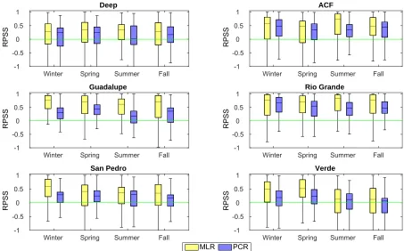
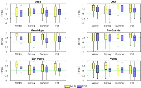
forecasts in a seasonal time scale. . . 20 Figure 1.3 Comparison of MLR and PCR models performances on split sample

forecasts in a seasonal time scale. . . 21 Figure 1.4 Comparison of skill in individual streamflow forecasts between the

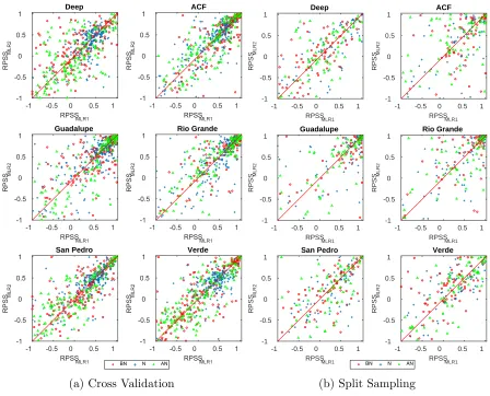
models MLR1 and MLR2 . . . 24 Figure 1.5 Cloud plot comparison of skill in streamflow forecasting for Below

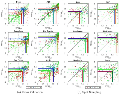
Normal (BN), Normal (N), and Above Normal (AN) months between the MLR model and PCR model under both cross-validation and split sample validation. The median lines of the cloud points are projected on each axes for each category. . . 25 Figure 1.6 Difference between MLR and PCR performances (∆RP SS =RP SSM LR−

RP SSP CR) with respect to the skewness of monthly streamflows for all the selected basins during Winter season. Positive ∆RP SS means MLR performs better than PCR. Significant positive relationship were found after fitting linear regression. . . 27 Figure 1.7 Decomposed contribution of probabilistic information from

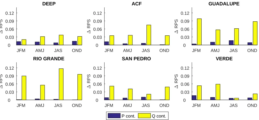
Precipita-tion forecasts (P) and antecedent streamflow observaPrecipita-tions (Q) as input variables in determining the skill of MLR streamflow forecasts under cross validation approach. . . 28 Figure 1.8 The performance range of MLR model in categorical streamflow

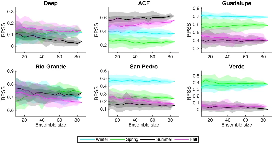
fore-casting as a function of ensemble size of precipitation forecasts during four seasons. The solid line, the darker area, and the lighter area in each color represents the median, IQR, and 90% confidence interval of the RPSSs respectively derived from 50 iterations at each ensemble size. 30

Figure 2.1 RRMSE of the bias corrected 1-3 months ahead soil moisture forecasts based on the SMAP soil moisture observations . . . 42 Figure 2.2 Correlation coefficient between 1-3 months ahead soil moisture forecasts

with the SMAP soil moisture observations. grid cells with insignificant correlations (based on 18 months of data) are grayed out . . . 42 Figure 2.3 Scatter plot of soil moisture residuals for two sample grid cells with

(13)

Figure 2.4 Comparison between the (a) NOAH3.2 retrospective 1 month ahead soil moisture forecasted percentiles with (b) the actual drought conditions from U.S. Drought Monitor (USDM) during historical drought of Oct 2007 . . . 45

Figure 3.1 Locations of the 857 selected HCDN stations across the 18 HUC level 2 geographical regions. HCDN basins are classified snow-melt and rainfall-runoff regimes based on the type of precipitation in influencing the runoff. . . 52 Figure 3.2 Performance of ’abcd’ model expressed as R-RMSE (first row) and

Pearson’s Correlation Coefficient (second row) in simulating observed flows over the CONUS. Grayed-out basins indicate high errors in simulated flows (R−RM SE >1) or insignificant correlation coefficient at 95% confidence level. . . 66 Figure 3.3 Differences in R-RMSE in simulating observed flows with EnKF and

without EnKF through ’abcd’ model. Positive (negative) values indicate the improvements (degradations) introduced to the simulated flows due to EnKF. . . 67 Figure 3.4 Differences in R-RMSE in simulating observed low (high) flows due to

EnKF in ’abcd’ model shown in upper (lower) row. Low (high) flows correspond to months where the flows are lesser (greater) than the 10th (90th) percentile of climatology. Positive (negative) values in the figure indicate decreased (increased) error in simulations due to application of EnKF. . . 67 Figure 3.5 NSE in simulating observed flows through application of EnKF on state

variables (a) Soil moisture storage (St) and groundwater storage (Gt), (b) only groundwater (Gt), and (c) only soil moisture (St). Stations

with N SE <0 are not shown. . . 69 Figure 3.6 Seasonal R-RMSE (first row) and correlation (second row) in forecasting

observed monthly flows using ’abcd’ model (without EnKF) during four seasons. Stations with R-RMSE values greater than 1 or insignificant correlation coefficients (corresponding to 95% confidence level) are shown as gray. . . 70 Figure 3.7 Difference in R-RMSE (∆R-RMSE = R-RMSEabcd−RRMSEabcd−EnKF)

(14)

Figure 4.1 Location of the Tar River basin and USGS gauging station #02089500 located at Tarboro North Carolina . . . 82 Figure 4.2 Seasonality of Tar River Basin . . . 83 Figure 4.3 Schematic of the variational data assimilation approach. Black squares

represent the model states (not in the streamflow dimension), triangles are the streamflow observations, U F and AW denotes DA Update Frequency and Assimilation Window parameters respectively. The hydrologic model is then initialized using the state conditions achieved either from Open Loop (OL) simulation or Data Assimilated (DA) simulations. . . 87 Figure 4.4 Timeseries of monthly streamflow observations along with streamflow

simulations from Open Loop (OL) scheme and Data Assimilation (DA) experiment using U F = 15days and AW = 10days. . . 95 Figure 4.5 ∆KGE (KGEDA−KGEOL) Improvement in Streamflow Simulations

after applying VAR data assimilation for different AW andU F lengths using all flows (gray-scaled plots), only low flow analysis (i.e. observed streamflow less than 10th_percentile_{Q < Q}

p=0.1) (orange plots) and only

high flow analysis (i.e. observed streamflow more than 90th percentile

Q > Qp=0.9) (blue plots) during the period 1991-2010. The first row

shows the statistics quantified using daily flows and the second row plots are generated using average monthly flows. The skill of open-loop simulations for each of the analyses are shown in the plot titles in terms of KGE. . . 96 Figure 4.6 Timeseries of monthly forecasted streamflow acquired from both

de-terministic and probabilistic forecasting approaches. Prior to monthly forecasting VIC model is initialized either based on Open Loop (OL) states (first row) or through Data Assimilated (DA) initial conditions (second row) using AW = 15days. . . 98 Figure 4.7 The magnitude of the model skill improvements due to data assimilation

over daily time steps of a monthly prediction. Each color represents the DA application with a unique assimilation window length AW. . 102 Figure B.1 Evaluation of Spearman’s rank correlation between downscaled monthly

precipitation forecasts and observed precipitation at 1/8◦ grid cells over Tar River basin, NC. . . 147 Figure B.2 Timeseries of optimal scale factor K for various DA experiments with

different U F and AW parameters. Y axis of the plots are limited between 0 and 2, with the middle thick sign showing the value 1 for the

(15)

Figure B.3 Mean and Variance of K multiplier computed during 20 years of simulations for various DA experiments with different U F and AW

(16)

INTRODUCTION

Water resources management at monthly-to-seasonal time scales typically requires 1-month to 3-month ahead hydrologic forecasts such as streamflow and soil moisture attributes. Over last decades, considerable progress have been made in understanding the low-frequency climate variability and its impact on developing seasonal hydrologic forecasts. Yet, the quality of forecasts has not been improved substantially for practical applications, hence the necessity of understanding potential strategies for improving and advancing uncertainty reduction methods in the streamflow forecasting from multiple error sources [Welles et al., 2007]. Mainly, the streamflow dynamics in a catchment depend on two major influential components: 1) atmospheric conditions over the watershed and 2) land surface states (e.g. soil moisture, snow cover, etc.) which is also known as Initial Hydrologic Conditions (IHCs). Seasonal climate forecasts are routinely issued by climate prediction centers. Given the atmospheric forcings, realistic estimates of initial hydrologic conditions is critically required especially for seasonal hydrologic predictions, although they are hard to be acquired or measured directly. Furthermore, other sources of uncertainty involved in hydrologic predictions such as model and parameter uncertainties also degrade the skill in streamflow predictions. In this regard, substantial effort have been made in order to reduce the prediction errors due to parameter uncertainty as well as hydrologic model uncertainty [Beven and Binley, 1992; Vrugt et al., 2003; Wilby, 2005; Li et al., 2015].

(17)

However, current precipitation and temperature forecasts are still not reliable at seasonal time scales, which is a critical time scale for management purposes. The predictability of climate systems especially for seasonal lead times relies on boundary conditions, particularly sea surface temperature (SST) [Lorenz, 1993]. Thus a better understanding of climatic variability (e.g. El Nino-Southern Oscillation-ENSO) can lead to more accurate seasonal climate forecasts. Reducing uncertainty in climate models and forcings through multimodel combination of climate forecasts will also reduce uncertainty in streamflow forecasts [Devineni et al., 2008; Devineni and Sankarasubramanian, 2010b; Li et al., 2016]. In addition, better estimation of soil moisture state enhance the prediction skill in numerical climate models [Fennessy and Shukla, 1999].

(18)

Outline of the Dissertation

In this dissertation, different methods of developing land-surface attributes (i.e. streamflow and soil moisture) for medium-range lead times (e.g. monthly to seasonal) are employed and tested along with the quantification of the uncertainty in the forecasted products through various statistical analyses and verification metrics. and then try to quantify the uncertainty in probabilistic forecasts of streamflow and deterministic forecasts of soil moisture. Furthermore, with the intention of reducing error in land-surface state, data assimilation techniques are applied into different types of hydrologic models and the enhancements in the model products are assessed and presented.

(19)

Chapter

1

Utilizing Probabilistic Downscaling

Methods to Develop Streamflow

Forecasts from Climate Forecasts

Abstract

(20)

1.1. INTRODUCTION CHAPTER 1. PROBABILISTIC DOWNSCALING

exhibit higher Rank Probability Skill Score (RPSS) compared to the PCR probabilistic forecasts. MLR forecasts are also more skillful than PCR forecasts during the winter season and for basins that exhibit high interannual variability in streamflows. The role of ensemble size of precipitation forecasts in developing MLR-based streamflow forecasts was also investigated. Given the simplicity involved in MLR, it offers an alternate reliable approach in developing categorical streamflow forecasts.

1.1 Introduction

(21)

models to develop multimodel ensemble which reduces the model uncertainty [Ajami et al., 2006;Li and Sankarasubramanian, 2012;Devineni et al., 2008].

Statistical model forecasting is based on developing a statistical relationship between relevant climatic predictors and/or some available observations such as initial soil moisture and streamflow conditions prior to the forecasting. Commonly, statistical models such as Principal Component Regression (PCR) assumes normality of predictands and linearity between predictors and predictands [Hsu et al., 1995; Garen, 1992; Sankarasubramanian et al., 2008]. However it is well-known that nonlinear relationship exists between runoff and precipitation [Jakeman et al., 1993; Sankarasubramanian and Vogel, 2003]. For a long time, considerable progress has been made on incorporating the influence of Sea Surface Temperature (SST) anomalies such as El Nino Southern Oscillation (ENSO), which partially holds information in tropics and subtropics towards seasonal precipitation and streamflow forecasting [Ropelewski and Halpert, 1986;Tootle et al., 2005; Hamlet and Lettenmaier, 1999]. In addition to SST anomalies, statistical models can benefit from the natural persistence of streamflow in order to improve their forecasting skill through using information of past streamflow conditions. Previous studies have employed various types of statistical modeling techniques including parametric, semi-parametric and re-sampling methods (e.g. K-Nearest Neighbors (K-NN), Model Output Statistics (MOS), etc. ) in order to develop probabilistic streamflow forecasts over a specific watershed or across a region [Grantz et al., 2005;Clark and Hay, 2004].

(22)

than that of climate forecasts issued from GCMs. Addressing this resolution mismatch is a big challenge in itself and requires the application of spatial downscaling and/or temporal disaggregation approaches on GCM outputs before forcing them into hydrologic models [Wood et al., 2002; Wood and Lettenmaier, 2006; Yuan et al., 2011]. In addition, both downscaling and disaggregation procedures introduce errors into the climatic forcings and subsequently hydrologic products; thus might significantly influence the reliability of streamflow forecasts, mostly depending on their location and forecasting season. [Mazrooei et al., 2015;Sinha et al., 2014; Seo et al., 2016].

Climate forecasts, that are available in large spatial scales, are typically issued in the form of ensembles, which quantify the uncertainty due to the initial conditions [Goddard et al., 2003;Doblas-Reyes et al., 2005]. Various studies have focused on reducing uncertainty in climate forecasts by combining multiple models [Barnston et al., 2003; Weigel et al., 2008] and developing different strategies for providing ensembles that quantify uncertainty in atmospheric conditions [Kumar et al., 2001;Li et al., 2008] and hydrologic states [Shukla and Lettenmaier, 2011]. However, for statistical downscaling, most studies used only the ensemble mean of climate forecasts for developing streamflow forecasts which ignores the probabilistic information in the data [Sinha and Sankarasubramanian, 2013]. Few studies that pointed out the significance of these probabilistic information use ensemble spread or a subset of skillful ensemble members in their modeling process in order to gain more accuracy in the forecasted products [Wilks and Hamill, 2007; Regonda et al., 2006].

(23)

information inside the large scale ensemble climate forecasts into basin-scale and utilize it for probabilistic streamflow forecasting. Unlike binary logistic regression that deals with only two categories of events, MLR is able to develop categorical probabilities for multiple outcomes and predefined events. The other advantage of MLR is that the model input can be both probabilistic data such as probabilistic information derived from climate ensembles as well as deterministic data such as initial land surface conditions of a catchment. In this study, we have employed precipitation forecasts from ECHAM4.5 GCM along with past streamflow observations to build MLR model for developing 1-month ahead categorical streamflow forecasts over six river basins that span across various hydroclimatic regimes located in the US Sunbelt. The performance of MLR model was then compared with the commonly used PCR model in order to identify the added value of using probabilistic information in the ensemble climate forecasts for improving streamflow forecasts. Results from our experiments address the following science questions associated with categorical streamflow forecasting:

1. How is the MLR model performance compared to PCR model in developing proba-bilistic categorical streamflow forecasts during different seasons?

2. What is the information added to the categorical streamflow forecasts developed using the MLR model?

3. Is there any relationship between the skill of MLR model and river basins’ charac-teristics and their regimes?

(24)

1.2. DATA CHAPTER 1. PROBABILISTIC DOWNSCALING

ACF River USGS#02358000

Deep River USGS#02102000

Guadalupe River USGS#08167500 Rio Grande River USGS#08276500

San Pedro River USGS#09471000 Verde River

USGS#09508500

— 37°N

Figure 1.1. Map of the US with the Sunbelt specified as the red shaded area as well as the location of the selected river basins and their considered USGS gauging stations

This manuscript is organized as follows: Section 1.2 provides information about the selected river basins and the hydroclimatic data used in this study. Section 1.3 details the MLR and PCR experimental setup and verification metrics used for model evaluations. Section 1.4 presents the results following with section 1.5 that summarizing the findings and conclusion from the study.

1.2 Study Area and Data

1.2.1 Study Area

(25)

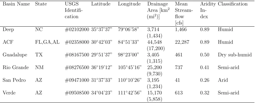
Table 1.1. USGS gauge sites characteristics

Basin Name State USGS Identifi-cation

Latitude Longitude Drainage Area [km2

(mi2_)]

Mean Stream-flow [cfs]

Aridity In-dex

Classification

Deep NC #02102000 35◦37’37” 79◦06’58” 3,714 (1,434)

1,466 0.89 Humid

ACF FL,GA,AL #02358000 30◦_42’03” ₈₄◦_51’33” _44,548

(17,200)

22,287 0.89 Humid

Guadalupe TX #08167500 29◦_51’37” ₉₈◦_23’00” _3,405

(1,315)

461 0.50 Dry sub-humid

Rio Grande NM #08276500 36◦_19’12” ₁₀₅◦_45’16” _25,200

(9,730)

737 0.41 Semi-arid

San Pedro AZ #09471000 31◦37’33” 110◦10’26” 3,195 (1,234)

41 0.26 Arid

Verde AZ #09508500 34◦_04’23” ₁₁₁◦_42’56” _15,170

(5,858)

613 0.32 Semi-arid

Table 1.1 presents detailed information about the selected river basins and their streamflow gauge stations.

1.2.2 Streamflow Data

(26)

1.2.3 Climate Forecasts

Precipitation forecasts from ECHAM4.5 GCM model was obtained from International Research Institute of Climate and Society (IRI) data library [Li and Goddard, 2005]. ECHAM model is developed by Max Planck Institute and is currently used in real time climate forecasting [Roeckner et al., 1992]. We considered ECHAM4.5 since it has a long period of retrospective monthly precipitation forecasts and studies have shown that ECHAM4.5 precipitation forecasts can provide a reliable skill in streamflow forecasting [Mazrooei et al., 2015; Sinha et al., 2014]. In this study we used both ECHAM4.5 monthly simulations and monthly forecasts both available at 2.8◦×2.8◦ _{resolution. In the simulation}

(27)

1.3. METHODOLOGY CHAPTER 1. PROBABILISTIC DOWNSCALING

1.3 Methodology

For each river basin, the grid point of ECHAM4.5 precipitation forecasts having the highest correlation with the observed streamflow was selected among all the grid points that overlay or neighbor the basin boundary. Then the precipitation forecasts from the selected grid point and the observed monthly streamflow prior to the forecasting time step were considered as the two predictors of our modeling framework, along with the observed streamflow in that forecasting month considered as the predictand variable. Two models, Multinomial Logistic Regression (MLR) and traditional Principal Component Regression (PCR) were considered to develop streamflow forecasts. The models were evaluated based on leave-5-out cross validation and split sample validation to develop probabilistic streamflow tercile forecasts. This section provides more details about both models and validation techniques.

1.3.1 Candidate Models

Principal Components Regression (PCR)

Climate Predictability Tool (CPT) from IRI [Mason and Tippett, 2016] was employed in order to develop the PCR model. For a given month, the predictor variables for the PCR model include the ensemble mean of the precipitation forecasts (µprec) and the previous month observed streamflow (Qt−1) and PCR model estimates the conditional

(28)

(_P(QBN),P(QN),P(QAN)) based on the climatological thresholds. PCR is one of the widely used Model Statistic Output (MOS) approaches in both hydrological research fields and operational forecasting frameworks [Antolik, 2000; Garen, 1992; Hamill et al., 2006;Pagano, 2008; Li et al., 2014; Arumugam et al., 2015]. However, the disadvantage of this method is that it only considers the ensemble mean and ignores the probabilistic information in the ensemble of climate forecasts.

Multinomial Logistic Regression (MLR)

Multinomial logistic regression is an extension of binary logistic regression, which enables the model to develop probabilistic predictions for multiple categories and outcomes. MLR is also capable of accepting inputs from mixed data types such as probabilities and deterministic variables. In order to feed MLR with the probabilistic information from the ensemble of climate forecasts, we quantified the probability of below normal _P(PBN), normal _P(PN), and above normal P(PAN) precipitation forecasts. For this purpose, we first pooled together all the forecasted precipitation ensembles over the study period (1957-2002) for a given month and then the 33rd and 67th model climatological percentiles were computed. Based on these climatological statistics of the ECHAM4.5 GCM, we estimated the probabilities of categorical precipitation forecasts in two different ways:

(i) Bin Counting: For each time step, the number of ensemble members that fall between the GCM model climatological 33rd _{and 67}th _{percentiles were counted and then}

(29)

probabilistic predictors.

(ii) Distribution Fitting: For each time step, a log-normal distribution was fit to the precipitation ensemble and the CDF of the model climatological 33rd and 67th quantiles were computed. MLR model fed with this type of predictor is called

MLR2 in the following.

The predictor matrix X ( Eqn. 1.1 ) for MLR model consists of probabilities of categorical precipitation events as well as observed streamflow prior to the forecasting time step. We didn’t include _P(PAN) in the predictors since it can be derived from the other two probabilities thus it doesn’t add any additional information into the modeling framework. MLR model requires categorized outcomes as the predictand, thus for a given month we converted the streamflow observations to nominal outcomes based on the 33rd and 67th quantiles of the historical records. The MLR model then estimates the coefficient matrix B ( Eqn. 1.2 ) for the regression. In MLR model, number of rows in the coefficient matrix should be equal to number of predictors plus one and number of columns is equal to number of outcome categories minus one so in our study the matrix B would have 4 rows and 2 columns. Finally based on the equations 1.3 and 1.4 and the rule that probabilities sum up to 1, the probabilities of the BN, N, and AN categories of streamflow forecasts were computed.

Xt=

P(PBN)t P(PN)t Qt−1

(30)

B =



       

B01 B02

B11 B12

B21 B22

B31 B32 

       

4×2

(1.2)

ln(P(QBN)

P(QAN)

) = B01+B11P(PBN) +B21P(PN) +B31Qt−1 (1.3)

ln( P(QN)

P(QAN)

) =B02+B12P(PBN) +B22P(PN) +B32Qt−1 (1.4)

1.3.2 Model Calibration and Validation

MLR and PCR models were conducted and evaluated based on two different validation techniques which are explained here.

1.3.2.1 Cross Validation

(31)

1.3.2.2 Split Sample Technique

In the split sample technique, unlike the cross-validation only a single subset of data is used to train the models. Here, The first 26 years of data (from 1957 to 1982) is used as the calibration period and the remaining 20 years (from 1983 to 2002) as the validation period.

Each of the explained validation techniques has its own advantages and drawbacks. Cross validation can stabilize the structure of the model since it uses different subsets of training data. On the other hand, in the split sample test the model has lesser years for the calibration and it is shown that it has lesser skill too, comparing to cross-validated forecasts [Goutte, 1997; Moradkhani et al., 2004]. Split sample test is commonly used and beneficial when there is a short set of dataset so it is not rational to leave out the available data. In addition, the split sample validation technique provides a more rigorous way to evaluate the skill of the model towards operational forecasting as it only uses past data to develop the forecasts [Klemeˇs, 1986].

1.3.3 Forecasting Skill Metrics

(32)

each time step and then RPSS is computed by comparing the RPS of forecast with the RPS of climatology (Eqn. 1.7),

RP St = 1

K

X

k=1

[_Pk_t −_Ok t]

2 _(1.5)

RP S_tclimatology = 1

K

X

k=1

[ ¯_Ok−_Ok t]

2 _(1.6)

RP SSt= 1−

RP St

RP S_tclimatology (1.7)

where in the above equations, _Pk

t, Okt, and ¯Okt are the forecasted, observed, and climatological cumulative probabilities respectively at the time step t for the kth _category.

In addition to RPSS, in order to diagnose different attributes of the forecasting skill for a specific category (e.g. BN or AN), we employed commonly used Brier Score (BS) [Brier, 1950; Weigel et al., 2007], and its empirical decomposition into reliability (REL), resolution (RES), and uncertainty (UNC) were quantified for model intercomparison purposes based on the following equations:

BS = 1

N

X

t=1

(pt−yt)2 (1.8)

BS =REL−RES+U N C (1.9)

REL= D X d=1 nd N( od nd

−Pd)2 (1.10)

RES = D X d=1 nd N( od nd

(33)

1.4. RESULTS CHAPTER 1. PROBABILISTIC DOWNSCALING

U N C = ¯o(1−o¯) (1.12)

where N is total number of forecast probabilities, yt is binary observation (yt = 1 if event happened and yt = 0 otherwise), and the issued forecasts pt were assumed to have D distinct values (i.e.pt ∈ {P1, ..., PD}) for all timesteps t. nd denotes the number of times when the dth _{forecast was issued, and} _o

d refers to the total number of events that have been observed when the dth _{forecast was issued. ¯}_o _{is the climatological event}

frequency which is equal to 0.33 (i.e. BN or AN months) in this case.

1.4 Results

(34)

indicating a higher uncertainty in streamflow forecasts. MLR performs better than PCR in the Guadalupe river basin during the winter season with the first quartile of MLR being approximately above the third quartile of PCR highlighting that in 75% of occasions MLR would be more skillful.

Fig. 1.3 shows the same analysis of RPSS values developed under the split-sample validation technique. We again see that both MLR and PCR forecasts are more skillful than the climatology. Comparing the RPSS median between the two forecasting models, MLR model still performs better than the PCR model in all basins over all seasons with just one exception during spring season in the Deep river basin. From Fig. 1.2 and Fig. 1.3 we notice that the skill of cross-validated forecasts vary less in comparison to the split-sample validation. The reason is that the cross-validation approach considers more data for model training resulting in less variability in model skill. We also notice under both validation techniques that MLR model’s distributions of RPSSs are more skewed towards higher values indicating that MLR is able to issue better streamflow predictions over the considered period suggesting higher reliability of MLR.

(35)

Winter Spring Summer Fall

-1 -0.5 0 0.5 1 RPSS Deep

-1 -0.5 0 0.5 1 RPSS ACF

-1 -0.5 0 0.5 1 RPSS Guadalupe

-1 -0.5 0 0.5 1 RPSS Rio Grande

-1 -0.5 0 0.5 1 RPSS San Pedro

-1 -0.5 0 0.5 1 RPSS Verde MLR PCR

(36)

-1 -0.5 0 0.5 1 RPSS Deep

-1 -0.5 0 0.5 1 RPSS ACF

-1 -0.5 0 0.5 1 RPSS Guadalupe

-1 -0.5 0 0.5 1 RPSS Rio Grande

-1 -0.5 0 0.5 1 RPSS San Pedro

-1 -0.5 0 0.5 1 RPSS Verde MLR PCR

(37)

Table 1.2. Improved forecast attributes (positive/bold values) in terms of ∆BS =

BSP CR−BSM LR, ∆REL= RELP CR−RELM LR, and ∆RES =RESM LR−RESP CR, by utilizing MLR forecasts over PCR forecasts for BN and AN months

BN AN

∆BS ∆REL ∆RES ∆BS ∆REL ∆RES

Basin [×10−2 ] [×10−2 ] [×10−2 ] [×10−2 ] [×10−2 ] [×10−2 ]

Deep 2.35 -0.43 2.86 0.22 -0.52 0.84

ACF 1.82 1.40 0.64 -0.26 -0.35 0.26

Guadalupe 6.36 2.13 4.43 3.51 0.89 2.71

Rio Grande 2.97 1.13 1.87 0.37 0.03 0.48

San Pedro 2.72 -0.05 2.86 2.26 0.73 1.92

Verde 3.13 -0.36 3.55 2.23 1.20 1.60

have lower brier score for BN months and most likely for AN months over all the basins. This is particularly because of the greater resolution in MLR forecasts, thus containing more information compared to PCR forecasts (an ’uninformed’ forecaster has RES = 0). However, ∆REL values imply that sometimes MLR has lower reliability (a reliable forecaster has REL= 0) compared to PCR, but this degradation is dominated by the improved resolution and eventually results in better (lower) brier score.

(38)

points are scattered almost equally on the two sides of the diagonal line indicating no significant difference in forecasting skill whether using bin counting or fitting a log-normal distribution to the precipitation ensemble.

Fig. 1.5 demonstrates the comparison between the skill of MLR and PCR models in categorical streamflow forecasting for each individual monthly time step during the validation period. In order to simplify the comparison across the models, the medians of the RPSS values for each category were shown on each axes as colorized lines. In this figure, since the majority of points and consequently the intersection of median lines are located below the diagonal line, it indicates that the RPSS of MLR is higher than PCR. By looking at the point clouds in Fig. 1.5a we see that the skill of PCR model varies less (less deviation in RPSS values) in terms of forecasting normal (N) flows compared to other two categories. MLR model performs more precisely in arid regions like Guadalupe and Rio Grand river basins, since most of the points are scattered on the right side of the boxes. Based on the medians of the RPSSs in Fig. 1.5a, both MLR and PCR models have a better skill in forecasting AN and BN months, compared to N months. It is harder to conclude this by looking at Fig. 1.5b since there are fewer data points in the split sample validation as we have limited sample size under the different flow categories. In addition, the better performance of MLR is distinct in the arid basins.

Further, the seasonal relationship between the mean monthly ∆RP SS (∆RP SS =

RP SSM LR−RP SSP CR) and the skewness of monthly flows, γ based on Eqn. 1.13:

γm =

E(Qm−Q¯m)3

σ3

Qm

(1.13)

(39)

-1 -0.5 0 0.5 1 RPSS_MLR1 -1 -0.5 0 0.5 1 RPSS MLR2 Deep

-1 -0.5 0 0.5 1 RPSS_MLR1 -1 -0.5 0 0.5 1 RPSS MLR2 ACF

-1 -0.5 0 0.5 1 RPSS_MLR1 -1 -0.5 0 0.5 1 RPSS MLR2 Guadalupe

-1 -0.5 0 0.5 1 RPSS_MLR1 -1 -0.5 0 0.5 1 RPSS MLR2 Rio Grande

-1 -0.5 0 0.5 1 RPSS_MLR1 -1 -0.5 0 0.5 1 RPSS MLR2 San Pedro

-1 -0.5 0 0.5 1 RPSS_MLR1 -1 -0.5 0 0.5 1 RPSS MLR2 Verde

BN N AN

(a) Cross Validation

-1 -0.5 0 0.5 1 RPSS_MLR1 -1 -0.5 0 0.5 1 RPSS MLR2 Deep

-1 -0.5 0 0.5 1 RPSS_MLR1 -1 -0.5 0 0.5 1 RPSS MLR2 ACF

-1 -0.5 0 0.5 1 RPSS_MLR1 -1 -0.5 0 0.5 1 RPSS MLR2 Guadalupe

-1 -0.5 0 0.5 1 RPSS_MLR1 -1 -0.5 0 0.5 1 RPSS MLR2 Rio Grande

-1 -0.5 0 0.5 1 RPSS_MLR1 -1 -0.5 0 0.5 1 RPSS MLR2 San Pedro

-1 -0.5 0 0.5 1 RPSS_MLR1 -1 -0.5 0 0.5 1 RPSS MLR2 Verde

BN N AN

(b) Split Sampling

(40)

-1 -0.5 0 0.5 1 RPSS_MLR -1 -0.5 0 0.5 1 RPSS PCR Deep

-1 -0.5 0 0.5 1 RPSS_MLR -1 -0.5 0 0.5 1 RPSS PCR ACF

-1 -0.5 0 0.5 1 RPSS_MLR -1 -0.5 0 0.5 1 RPSS PCR Guadalupe

-1 -0.5 0 0.5 1 RPSS_MLR -1 -0.5 0 0.5 1 RPSS PCR Rio Grande

-1 -0.5 0 0.5 1 RPSS_MLR -1 -0.5 0 0.5 1 RPSS PCR San Pedro

-1 -0.5 0 0.5 1 RPSS_MLR -1 -0.5 0 0.5 1 RPSS PCR Verde

BN N AN

(a) Cross Validation

-1 -0.5 0 0.5 1 RPSS_MLR -1 -0.5 0 0.5 1 RPSS PCR Deep

-1 -0.5 0 0.5 1 RPSS_MLR -1 -0.5 0 0.5 1 RPSS PCR ACF

-1 -0.5 0 0.5 1 RPSS_MLR -1 -0.5 0 0.5 1 RPSS PCR Guadalupe

-1 -0.5 0 0.5 1 RPSS_MLR -1 -0.5 0 0.5 1 RPSS PCR Rio Grande

-1 -0.5 0 0.5 1 RPSS_MLR -1 -0.5 0 0.5 1 RPSS PCR San Pedro

-1 -0.5 0 0.5 1 RPSS_MLR -1 -0.5 0 0.5 1 RPSS PCR Verde

BN N AN

(b) Split Sampling

Figure 1.5. Cloud plot comparison of skill in streamflow forecasting for Below Normal (BN), Normal (N), and Above Normal (AN) months between the MLR model and

(41)

46 years of observations, were computed. This assessment was conducted by fitting a linear regression to the monthly data collected from all the basins during each season. Based on this seasonal analysis, we infer that a significant positive relationship between ∆RP SS and γ exists only in the winter season during which the estimated regression slope is greater than zero with the p-values less than 0.05 under both cross validation and split sample validation (Fig. 1.6). It is well known that climate models show more skill in forecasting during the winter season across the Southern US due to the teleconnections associated with ENSO conditions [Devineni and Sankarasubramanian, 2010b; Oh and Sankarasubramanian, 2012]. In addition, the selected basins also exhibit increased inter-annual variability in winter flows resulting in higher variations in skewness.

Similar analysis was also conducted based on monthly average ∆RP SS for each basin. Results showed that Deep and Rio Grande river basins exhibit a significant positive relationship between monthly ∆RP SS and γm. This suggests that MLR model performs better than PCR model in forecasting mode when skewness of monthly flows are higher, which typically occurs with higher inter-annual variability in streamflows. The improved performance of basins with high skewness also arises from the ability of MLR model to accommodate skewed nature of streamflow forecasts, whereas the PCR model assumes log-normal distribution, which forces the skewness of the streamflow forecast to be fixed (γ is zero in the log-transformed plane butγ = 3CV +CV3 _{in the original plane, where}

(42)

Figure 1.6. Difference between MLR and PCR performances (∆RP SS =RP SSM LR−

RP SSP CR) with respect to the skewness of monthly streamflows for all the selected basins during Winter season. Positive ∆RP SS means MLR performs better than PCR. Significant positive relationship were found after fitting linear regression.

Relative Contribution of Model Inputs

As mentioned earlier, the MLR model is forced with probabilistic information from precipitation forecasts along with deterministic streamflow observation from prior months. To further understand the role of each input component in determining the skill of probabilistic streamflow forecasting, MLR modeling was performed under two scenarios -the first one being probabilistic information from precipitation forecasts M LR(P) alone as a predictor, and the second being the antecedent streamflow observations M LR(Qt−1)

alone as a predictor - for developing streamflow forecasts. The forecasted products from these schemes were then compared to the original MLR modeling scheme which uses both input variables (M LR(P, Qt−1)) and were evaluated based on the differences in

(43)

JFM AMJ JAS OND

0 0.03 0.06 0.09 0.12 " RPS DEEP

JFM AMJ JAS OND

0 0.03 0.06 0.09 0.12 " RPS ACF

JFM AMJ JAS OND

0 0.03 0.06 0.09 0.12 " RPS GUADALUPE

JFM AMJ JAS OND

0 0.03 0.06 0.09 0.12 " RPS RIO GRANDE

JFM AMJ JAS OND

0 0.03 0.06 0.09 0.12 " RPS SAN PEDRO

JFM AMJ JAS OND

0 0.03 0.06 0.09 0.12 " RPS VERDE

P cont. Q cont.

Figure 1.7. Decomposed contribution of probabilistic information from Precipitation forecasts (P) and antecedent streamflow observations (Q) as input variables in deter-mining the skill of MLR streamflow forecasts under cross validation approach.

between each of the scenarios and the original modeling scheme, which basically denotes the role of the input component that was excluded from each scenario. For instance, the comparison between M LR(Qt−1) and M LR(P, Qt−1) schemes quantifies the contribution

(44)

Ensemble Size Analysis

(45)

1.5. DISCUSSION CHAPTER 1. PROBABILISTIC DOWNSCALING

20 40 60 80

RPSS 0 0.1 0.2 0.3 Deep

20 40 60 80

RPSS

0.2 0.4 0.6

ACF

20 40 60 80

RPSS 0.3 0.4 0.5 0.6 0.7 0.8 Guadalupe Ensemble size

20 40 60 80

RPSS

0.6 0.7 0.8

0.9 Rio Grande

Ensemble size

20 40 60 80

RPSS 0.1 0.2 0.3 0.4 0.5

0.6 San Pedro

Ensemble size

20 40 60 80

RPSS 0 0.1 0.2 0.3 0.4 0.5 Verde

Figure 1.8. The performance range of MLR model in categorical streamflow forecasting as a function of ensemble size of precipitation forecasts during four seasons. The solid line, the darker area, and the lighter area in each color represents the median, IQR, and 90% confidence interval of the RPSSs respectively derived from 50 iterations at each ensemble size.

1.5 Discussion and Concluding Remarks

(46)

the probabilistic information in climate forecasts and previous month streamflow. Thus, coarse-scale ensemble-based precipitation forecasts from ECHAM4.5 GCM along with past observations of streamflow from HCDN dataset were used as the predictors of MLR model in order to issue 1-month ahead streamflow forecasts consisted of Below Normal (BN), Normal (N), and Above Normal (AN) streamflow occurrences over six river basins across the US Sunbelt. We compared the performance of MLR model with the traditional approach, Principal Component Regression (PCR), which is commonly used to obtain the categorical precipitation and streamflow forecasts. Our findings demonstrated that MLR and PCR models both have a higher forecasting skill than climatology for almost all the seasons by having the median of RPSS values greater than zero. Also, the analysis of both models under cross validation and split sample validation techniques revealed that the MLR model has a higher skill in producing categorical streamflow forecasts comparing to traditional regression alternatives such as the PCR model. The reason is that the MLR model is capable of utilizing the probabilistic information in the climate forecast ensemble while the PCR model is built based on the mean of the ensembles, thereby not considering the ensemble spread in issuing categorical forecasts. Further, MLR structure is based on the multinomial distribution, which can naturally accommodate the skewness exhibited in the conditional distribution of flows. Hence, MLR model performs more accurately in arid basins and during months with high skewness in flows over humid basins.

(47)

potentially consider snow water equivalent (SWE) as a predictor instead of streamflow records particularly for predictions during the melting seasons. However, for non snowmelt months, considering antecedent streamflow would be a good strategy to develop monthly streamflow forecasts. For basins under rainfall-runoff regime, consideration of additional predictors such as remotely-sensed soil moisture products (e.g. SMAP) and groundwater levels (e.g. from USGS Climate-Groundwater Response Network) could also be given to en-hance the forecasting skill. Even though this study shows the contribution of precipitation forecasts in improving the skill is limited, one could also consider tercile forecasts from multi-model ensemble which in general improves the reliability of climatic probabilistic forecasts [Devineni and Sankarasubramanian, 2010a; Singh and Sankarasubramanian, 2014]. We also infer that the skill of the streamflow forecasts in general improves for large basins in comparison to the smaller basins. For instance, Deep River basin has relatively the lowest skill compared to the rest of the basins. Thus, basins dominated with significant groundwater storage (e.g., ACF) having strong persistence in streamflows are expected to have its’ skill contributed mostly by previous month streamflow conditions.

In this study, two different methods were employed and evaluated to estimate the probabilistic information inside the climate forecasts. The MLR model was forced with tercile precipitation forecasts estimated either by(1)counting the ensemble members lies in each category or by (2)_{fitting a log-normal distribution to the forecasted ensembles.}

(48)

members are enough to estimate streamflow forecasts while further increase in ensemble size did not result in any significant and consistent improvements in the skill of categorical streamflow forecasting. Thus, the proposed MLR approach offers an alternate approach to issue categorical streamflow forecasts that are typically needed in communicating the change in monthly/seasonal streamflow potential.

acknowledgments

(49)

Chapter

2

Comparison of NOAH3.2

Monthly-to-Seasonal Soil Moisture

Forecasts with SMAP Satellite

Observations over the Southeast US

Abstract

(50)

2.1. INTRODUCTION CHAPTER 2. SM FORECASTING

forecasts with the retrospective 18-month comparison showing a statistically significant correlations of 0.62, 0.57, and 0.59 over 1-3 month lead times respectively. Comparison of the SM forecast with the 2007-2008 monitored drought indexes also indicate potential in issuing SM forecasts to support agricultural planning and operations.

2.1 Introduction

Seasonal climate forecasts are very beneficial for short-term planning and management of water and agriculture systems [Li et al., 2014;Indeje et al., 2006; Sinha et al., 2014]. Most evaluation of climate forecasts has traditionally focused only on the skill in predicting precipitation and streamflow [Hoerling et al., 2009;Devineni et al., 2008]. Limited efforts have focused on the utility of climate forecasts for agriculture systems by evaluating the skill in predicting seasonal to interannual variability in crop yield [Indeje et al., 2006;

(51)

2.1. INTRODUCTION CHAPTER 2. SM FORECASTING

domain. SM observations using microwave remote sensing began in the late 1970s with the Scanning Multichannel Microwave Radiometer [Owe et al., 1992;Guha and Lakshmi, 2004] and continued with the Special Sensor Microwave Imager [Choudhury et al., 1990;Lakshmi et al., 1997a, b]. In the past decade with the launch of AMSR (Advanced Microwave Scanning Radiometer) [Njoku et al., 2003] there was a decade long dataset (2002-2011) for SM from space. This effort continued with the European Space Agency SMOS (Soil Moisture and Ocean Salinity Mission) [Kerr et al., 2012] and currently we have SMAP (Soil Moisture Active Passive Mission) [Entekhabi et al., 2010;Chan et al., 2016;Colliander et al., 2017; Ahmadalipour et al., 2017c]. The SMMR and AMSR were C band missions with a penetration depth of a few cm (less than 5), SSM/I - lowest frequency of 19 GHz (penetration depth around 12cm) and low spatial resolution (SSM/I 50km, AMSR

(52)

2.2. DATA AND METHODOLOGY CHAPTER 2. SM FORECASTING

with a brief discussion on the potential for issuing real-time M2S SM forecasts.

2.2 Hydroclimatic Data and Forecast Methodology

In this study, we used SMAP observations to validate the ability of NOAH3.2 LSM in forecasting SM at M2S time scales over the SEUS using the NASA’s Land Information System (LIS version 6.2) framework [Kumar et al., 2006]. Our forecasting scheme uses precipitation forecasts from ECHAM4.5 Atmospheric General Circulation Model (AGCM) along with climatology of meteorological variables (except precipitation) included in the phase 2 of the North American Land Data Assimilation System (NLDAS-2) dataset to implement the LSM.

2.2.1 SMAP

(53)

2.2.2 ECHAM4.5 Precipitation Forecasts

Monthly updated precipitation forecasts from ECHAM4.5 AGCM were obtained from the International Research Institute for Climate and Society (IRI) Climate Data Library [Li and Goddard, 2005]. The ECHAM4.5 climate forecasts are issued at a resolution of 2.8◦ from January 1957 with forecasts available up to 7-month lead time for every month consisting of 24 ensemble members. Constructed analogue Sea Surface Temperature (SST) forecasts have been used to develop the ECHAM4.5 AGCM climate forecasts. The spatio-temporal resolution of the climate forecasts is much coarser than the accepted resolution of the LSM forcing variables, thus statistical downscaling and disaggregation methods were employed in order to address this mismatch. We used the ensemble mean of monthly precipitation forecasts to spatially downscale from 2.8◦ to 1/8◦ by developing Principal Component Regression (PCR) with the observed precipitation available from

Maurer et al. [2002]. Following that, the downscaled monthly precipitation forecasts were temporally disaggregated to daily time scale using a Kernel nearest neighbor (K-NN) approach in order to develop 1-3 month ahead daily precipitation forecasts. Further details of spatial downscaling and temporal disaggregation methods can be found in Mazrooei et al.[2015].

2.2.3 NOAH3.2 LSM

(54)

coupled or uncoupled mode. NOAH3.2 is the version used in our study that requires near-surface atmospheric forcing as inputs and computes surface energy and water balance variables. NOAH3.2 is capable of developing output variables such as streamflow, soil moisture and soil temperature for various vertical layers, snowpack depth, snowpack water equivalent, canopy water content, and other energy flux and water flux terms [Ek et al., 2003]. The NOAH3.2 within the LIS6.2 was primarily used for developing the SM forecast.

2.2.4 Meteorological Forcings of LSM

The meteorological forcing (other than precipitation) for the NOAH LSM were acquired from the phase 2 of the North American Land Data Assimilation System (NLDAS-2) dataset [Mitchell et al., 2004]. NLDAS2 data is available at 1/8◦ spatial resolution and an hourly temporal scale from 1979 till present. We used the mean of these hourly forcings over a period of 31 years (1979-2010) in order to provide the meteorological forcing for the NOAH model. The initial land-surface conditions of the NOAH model were updated using the last hourly values prior to the forecasting time step.

2.2.5 Experimental Setup

(55)

were then used as ICs for the forecasting period. Under the forecasting mode, spatially downscaled and temporally disaggregated precipitation forecasts along with the hourly climatology of the NLDAS-2 forcing (excluding precipitation) and simulated end-of-the-month ICs were used to run NOAH3.2 LSM on a end-of-the-monthly basis to develop 3-end-of-the-month ahead monthly forecasts of SM. Mazrooei [2014b] used the above setup to develop streamflow forecasts for four target basins over the US Sunbelt. The resulted LSM products are at 0.25◦ spatial resolution and the domain of the modeling is set to Southeast US (defined as grid cells south of 37◦N latitude and east of 96◦W longitude).

(56)

2.3. RESULTS CHAPTER 2. SM FORECASTING

2.3 Results

Figure 2.1 (Figure 2.2) shows the RRMSE (correlation coefficient) between the bias-corrected SM forecasts and SMAP observations for 1-3 month lead time. Since we have only 18 data points, grids with insignificant correlations at 95% confidence interval (±1.96/√n, wheren = 18) are plotted in gray scale. As expected, the forecasting error increases from 1-month to 3-month lead time, but the spatial patterns in RRMSE remains the same with increase in lead time. The spatially averaged RRMSE over southeast were equal to 0.040, 0.042 and 0.041 for1-month, 2-month and 3-month lead times respectively. Among all the 1055 grid cells covering our study domain, only 23% of the grid cells, mostly located in the southeast side of Appalachian mountain, showed consistent increase in RRMSE. This minimal change in RRMSE can be associated with the strong memory (persistence) of SM during seasonal lead times [Koster et al., 2010]. From Figure 2.1, higher RRMSE occur over regions with predominantly wetland soil (e.g. Mississippi) and over regions with low content of clay abundant soil with slight swelling potential according toOlive et al. [1989] (e.g. east half of NC and SC states).

(57)

1-month ahead 2-month ahead 3-month ahead

0.01 0.02 0.03 0.04 0.05 0.06 0.07 0.08 0.09 0.1

Figure 2.1. RRMSE of the bias corrected 1-3 months ahead soil moisture forecasts based on the SMAP soil moisture observations

1-month ahead 2-month ahead 3-month ahead

0.1 0.2 0.3 0.4 0.5 0.6 0.7 0.8 0.9 1

(58)

Good Forecast

FCST RMSE =0.0704

(59)

the 18 months of SMAP observations.

To understand how the forecasts capture the variability in SMAP observations, two grid cells with high and low skill in forecasting were selected and anomalies around the mean of SMAP observations are presented (Figure 2.3). The first row shows a scatter plot between the anomalies of the forecasts and SMAP observations for a grid cell with relatively low RRMSE (0.019 on average) and strong correlation (0.726 on average) located in the east part of Georgia. The second row shows similar information for a grid cell located in SC with poor forecasting skill (high RRMSE and low correlation). Under good forecast, the model exhibits limited variability in forecasting below-normal anomalies (i.e., drought conditions) particularly for 2-month and 3-month lead times. For bad forecast, the model in general lacks ability to predict both anomalous conditions.

(60)

2.4. DISCUSSION CHAPTER 2. SM FORECASTING

Oct 2007

Forecasted Soil Moisture Percentiles

0 – 0.1 0.1 – 0.2 0.2 – 0.3 0.3 – 0.4 0.4 – 0.5 0.5 – 0.6 0.6 – 0.7 0.7 – 0.8 0.8 – 0.9 0.9 – 1

0.1 0.2 0.3 0.4 0.5

(a) NOAH3.2 Forecast

D0 Abnormally Dry D1 Moderate Drought D2 Severe Drought D3 Extreme Drought D4 Exceptional Drought

(b) USDM

Figure 2.4. Comparison between the (a) NOAH3.2 retrospective 1 month ahead soil moisture forecasted percentiles with (b) the actual drought conditions from U.S. Drought Monitor (USDM) during historical drought of Oct 2007

climatology. Comparing Figure 2.4a with the USDM drought monitoring conditions (from droughtmonitor.unl.edu) issued on Oct 16th _{2007 (Figure 2.4b), we see the 1-month ahead}

SM forecast captures the spatial pattern of drought severity indicating the hard-hit regions with lower percentiles of SM forecast. Thus, initializing the LSM with simulated NLDAS2 conditions and forcing the NOAH3.2 with ECHAM4.5 forecasted precipitation provides useful information for developing real-time M2S SM forecasts.

2.4 Discussion

(61)

2.4. DISCUSSION CHAPTER 2. SM FORECASTING

(62)

Chapter

3

Utilizing EnKF Data Assimilation in

Improving Monthly Streamflow

Forecasts over Contiguous US

Abstract

(63)

3.1. INTRODUCTION CHAPTER 3. ENKF DATA ASSIMILATION

variables of ”abcd” conceptual water balance model in order to forecast streamflow for 857 river basins across the conterminous United States (CONUS). Our results demonstrate that skill in predicting seasonal streamflow improves after EnKF application for most basins across the U.S. Sunbelt, whereas EnKF reduces the accuracy in streamflow prediction over snow dominated basins which is primarily due to the bias in snowmelt model. Also, EnKF improves low flow predictions, particularly during the summer season, resulting in 40% reduction in R-RMSE on average. Furthermore, the increased model skill due to EnKF was noticed under a streamflow forecasting, due to the enhancement of initial conditions even though the skill is predominantly dependent on the precipitation forecasts.

3.1 Introduction

Water balance models conceptually address the physical processes included in the trans-formation of the incoming precipitation - rainfall and snowmelt - into outflows such as evapotranspiration, groundwater recharge and runoff. These models are applied at daily to monthly time scales with different degrees of complexity representing the physical processes. Monthly water balance models were first introduced in the 1940s [Thornthwaite, 1948] and later modified in 1950s [Thornthwaite and Mather, 1955, 1957]. Such models are widely used in different research fields such as agricultural studies, climate impacts on streamflow, groundwater assessment, and watershed planning [Denmead and Shaw, 1962;

Alley, 1984; Vandewiele and Elias, 1995; Keshavarzi and Bakshi, 2012; Xu and Halldin, 1997; V¨or¨osmarty et al., 2000;Sankarasubramanian and Vogel, 2003].

(64)

hydrological modeling to quantify their impacts on model outputs [Kitanidis and Bras, 1980;Mazrooei et al., 2015; Sinha et al., 2014]. For instance, considerable effort has been made on improving the estimation of model parameters [Beven and Binley, 1992; Vrugt et al., 2003; Wilby, 2005]. Due to high nonlinearity and complexity of the watershed dynamics, it is a tough challenge to perfectly calibrate the models. Even if models are well-calibrated using manual/automatic calibration, the deficiency in the model structure will eventually cause mismatch between output and historical records [Ajami et al., 2004;

Moradkhani et al., 2005;Li and Sankarasubramanian, 2012]. Studies have explicitly focused on reducing the model uncertainty by optimally combining multiple model predictions [Hagedorn et al., 2005; Weigel et al., 2008; Singh and Sankarasubramanian, 2014; Yan and Moradkhani, 2016]. The multimodel combination approach is effective since it helps to overcome the spurious confidence of individual models and also reduces the propagated errors by optimal combination [Li et al., 2016; Kaiser Khan et al., 2014].

(65)

2016; Pham et al., 1998; Bertino et al., 2003]. However, application of DA in hydrological studies has started lately due to lack of suitable large-domain observations of initial states such as soil moisture as well as due to lack of proper quantification of the uncertainty both in observations and hydrologic models [Liu et al., 2012]. Nonetheless, the increasing availability of remotely-sensed observations of soil moisture and groundwater along with increased interest in real-time streamflow forecasting has made DA as an important step in streamflow prediction [Board et al., 2007].

The theory behind data assimilation relies on quantifying errors in the model pre-dictions and observations at the end of a timestep, and then updating the initial states based on the magnitude of error in predicting the precious timestep outputs. DA meth-ods are divided into two types: variational and sequential methmeth-ods. Variational data assimilation is more commonly used in numerical weather prediction whereas sequential data assimilation is used frequently in hydrological models since it works for distributed data sets [McLaughlin, 2002; Seo et al., 2003; Bertino et al., 2003]. Several sequential data assimilation algorithms have been introduced so far which are explained briefly in Appendix A.

Data assimilation in hydrological studies have focused on both lumped and distributed models with the purpose of improving model simulations [Moradkhani and Sorooshian, 2009]. In snow dominated catchments where the dynamics of stored snowpack plays an important role in streamflow predictions, assimilation of snow water equivalent (SWE) or snow cover extent (SCE) data has resulted in better performance of hydrological models [Sun et al., 2004; Slater and Clark, 2006; Lee et al., 2005; Liston and Hiemstra, 2008;

(66)

improves the estimation of land surface fluxes as well as error reduction in streamflow predictions [Pauwels et al., 2001; De Lannoy et al., 2007; Reichle, 2008; Montzka et al., 2011; Kumar et al., 2009]. Several studies reported the enhancement in operational short-term hydrological forecasting with the aid of assimilation of streamflow records in distributed models [Vrugt et al., 2006; R¨udiger et al., 2006; Clark et al., 2008]. A fundamental difference between assimilating variables such as soil moisture and snow observations with assimilating streamflow observations is the fact that in-situ records of streamflow are available over sufficient number of gauge stations for long time periods. On the other hand, ground measurements of snow and soil moisture content are hard and expensive to acquire, especially over a large spatial domain, and most of the DA studies tend to use remotely sensed data of these variables which covers a large domain, although it has short length of observations and contains large measurement errors. In addition, assimilation of the streamflow observation incorporates the information from the entire basin response and also captures the spatial variability within the watershed in generating the runoff. Hence, observed streamflow data could be used to update the state variables over previous time steps based on errors in streamflow predictions [Pauwels and De Lannoy, 2006].

Quantifying and Reducing Uncertainty from Multiple Sources in Forecasting Monthly to Seasonal Land-Surface Attributes.

ABSTRACT

DEDICATION

BIOGRAPHY

ACKNOWLEDGEMENTS

TABLE OF CONTENTS

LIST OF TABLES

LIST OF FIGURES

INTRODUCTION

Outline of the Dissertation

Chapter

1

Utilizing Probabilistic Downscaling

Methods to Develop Streamflow

Forecasts from Climate Forecasts

Abstract

1.1

Introduction

— 37°N

1.2

Study Area and Data

1.2.1

Study Area

1.2.2

Streamflow Data

1.2.3

Climate Forecasts

1.3

Methodology

1.3.1

Candidate Models

1.3.2

Model Calibration and Validation

1.3.3

Forecasting Skill Metrics

1.4

Results

Relative Contribution of Model Inputs

Ensemble Size Analysis

1.5

Discussion and Concluding Remarks

acknowledgments

Chapter

2

Comparison of NOAH3.2

Monthly-to-Seasonal Soil Moisture

Forecasts with SMAP Satellite

Observations over the Southeast US

Abstract

2.1

Introduction

2.2

Hydroclimatic Data and Forecast Methodology

2.2.1

SMAP

2.2.2

ECHAM4.5 Precipitation Forecasts

2.2.3

NOAH3.2 LSM

2.2.4

Meteorological Forcings of LSM

2.2.5

Experimental Setup

2.3

Results

0

0

0

0

0

0

0

0

0

0

0

0

Oct 2007

2.4

Discussion