Solution of Boundary and Mixed Problems in an Arbitrary Domain Using Fourier Transforms

(1)

Solution of Boundary and Mixed Problems in Arbitrary Domains Using Fourier Transforms

Gilnei Gonçalves Furtado

, Marco Túllio de Vilhena

, Telmo Roberto Strohaecker

and Rubem Panta Pazos

1) PPGEM/UFRGS, R. Oswaldo Aranha, 99, 6oandar, Porto Alegre / RS, 90035-190, Brazil, [email protected] 2) PPGEM/UFRGS, E-mail: [email protected]

3) PPGEM/UFRGS, E-mail: [email protected] 4) FAMAT/PUCRS, E-mail: [email protected]

ABSTRACT

In this work, we develop a method to solve partial differential equations in arbitrary domains by applying Fourier Transform technique. The main target of this work are the linear elastic problem. For such, the Fourier Transform technique is developed in domains with compact support, i.e. with the assumption that the unknown vanishes outside the domain. This approach establish an alternative procedure to determine the integral formulation for the boundary element method. We report solutions for the two-dimensional elastic linear equation.

INTRODUCTION

In a recent work Furtado, Vilhena and Strohaecker [1] proposed a closed-form solution for the general linear partial differ-ential equation with constant coefficients defined over a finite domain using the Fourier transform technique. Briefly speaking, the Fourier transform was applied to this problem, assuming that the solution vanishes outside the domain. After solving the transformed equation, the closed-form solution was obtained making the Fourier transform inversion.

In this work, we apply this approach to solve the two-dimensional linear elastic problem considering small strains, planar stress and isotropic material. To reach this goal, we outline the paper as follows: initially, we present the closed-form solution for the elastic problem. Afterward we report comments and simulation for the stress.

TWO-DIMENSIONAL LINEAR ELASTIC PROBLEM

We express the two-dimensional linear elastic problem considering small strains, planar stress and isotropic material, by the following partial differential equations

(1)

!

"

#

(2)

defined over an arbitrary finite domain$&%(' (figure (1)), where and are displacements in the and directions, and

and

are constants that depend on elastic material properties (

)

*

+-,! and

)

/.0,1 ,

2 is the modulus of elasticity and

3

is Poisson’s ratio) [2].

To solve this problem applying the Fourier Transform, we follow the idea of Furtado et al [1]. To this end, we begin with the application of the Fourier transform technique defined over finite domain in Eq. (1) and (2). It turns out:

54 687

4

9 ;:

=<

>

:

<

@?ACBEDF

HGJI *LKNM

+-OQPSR

TUBEDF

VGJI *LKNM

+-OQPSR

W

:

XBED

GYI *ZK[M

+\OQPSR

W

<

UB]D

GJI *ZKNM

+-OQP!^R

_B`D

aGJI *ZK[M

+-OQPQR

W

:`

b_B D

G I *LKNM

+-OQPR dc

"

:8<

?

_B DF

G I *ZKNM

+-OQP!R

W

:`

b_B`D

GJI *LKNM

+-OQPSR

XBED

eGJI *ZKNM

+-OQP!QR

UBED

fGJI *LKNM

+-OQPQR

W

<

=B D

G I *ZK[M

+\OQPR

W

:

UB D

G I *ZKNM

+-OQP!R

cag (3)

(2)

and

4 6 7

4

:

X<

>

:8<

?;XB D

G I *ZK[M

+\OQP R

TB D

VG I *ZK[M

+\OQP R

W

:

XB D

G I *ZKNM

+-OQP! R

W

<

TB D

G I *ZK[M

+-OQPR

"

_B D

aG I *ZK[M

+-OPR

W

:`

_B D

GJI *ZK[M

+-OPQR c

:

<

?

_B D

VGJI *ZK[M

+-OPQR

W

:`

T_B D

G I *ZK[M

+-OP

R

XB D

aG I *ZK[M

+\OQP

R

UB D

fG I *ZK[M

+-OP

R

W

<

=BED

GJI *LKNM

+-OQPSR

W

:

UBED

GYI *ZK[M

+\OQPQR

ceg (4)

For sake of simplification, we define the ensuing Fourier transformed functions

:

<

:

<

9 :

=<

(5)

:

<

:

<

9 :

=<

(6)

:

<

:8<

9 :

=<

(7)

Here we adopt the notation: ,

and

stand for the Fourier transform of the functions ,

and

. Furthermore,

,

M

and

P

denote partial derivatives respect to variables and .

c

b

A

B

Γ

a

C

D

x

y

d

Figure 1: Domain$ .

Next we perform the inverse Fourier transform of the functions , ,

,

M

and

P . For such, applying the

theorem of residue we get:

4

6

b]

(8)

4

6

&

(9)

4

6

&

(3)

P 6 (11) M 6 (12) P 6 (13)

On the other hand, integrating Eq. (8)—(13), we readily obtain the functions ,

and : 4 6 ? 6 6 c (14) 4 6 ?Q 6 6 c (15) 6 9 _ (16)

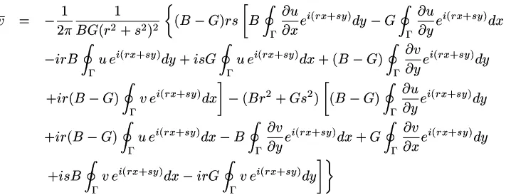
Now, we are in position to write down a closed-form solution for the problem (1)—(2). We reach this goal, making the Fourier inversion of and given by Eq. (3) and (4). This procedure leads to

54 687 > XBEDF R TB`DF R XB D R TB D R B D R B D R B DF R _B D M R B D R B D R XB D P R UBED M R g (17) and 4 6 7 > B D R B D R B D M R B D P R _B`D R _B D M R B D R " B D R =BED R UBED R =B D R UB D R g (18)

Recasting the above ansatz in matrix fashion we have

BED R BED R (19) where , and

(4)

(20) (21) (22)

and the vectors

and

have the entries

54 687 M !P M P P P !P M M M M P P P M P P M (23) 4 687 M P M M b M P M P M M b M P (24) evaluated at and . Here R

is given by

P R R M R R (25) and M P

are the director cosines of the normal to the contour of the domain.

Noticing that the boundary conditions are prescribed for the force intensity at boundary, we consider the ensuing relationship between M P M P and M P where M

P are the force intensities at boundary in the

and directions and

are tangential derivatives of and . Writing this relationship in matrix notation we have

(26)

where the matrix

has the entries

P M P M M P P 6 M 6 P M M P (27)

and the column vectors

, and

are given by

(28) M P (29) (30)

Replacing Eq. (26) in Eq. (19) we obtain

BED R BED . R (31) We define . (32) and rewrite

as block matrix

(33) where

is6 "!

matrix and

and

are6 6

matrices. Therefore, the Eq. (31), using this definition, has the form

B D$# % R B D R (34)

(5)

Next, we simplify the Eq. (34). For such using the result

B D

R

B D

R

(35)

combined with the definition

(36)

we quote the Eq. (34) as

B D R

B D

R

(37)

To this point it is important to remember that and

coincide with and

inside the domain$ and vanish outside the

domain$ .

In order to get the unknown boundary conditions for the and components of

and for the

M

and

P

components of

we proceed in similar manner as in Boundary Integral Method. In what follows, we briefly discuss this procedure:

1. We firstly begin expanding the components of

and in terms of some known basis functions;

2. We select a set of auxiliary points (positioned inside or outside the domain), where is the number of unknown

coefficients in the expansion of

and components. For more details see Furtado et all [1];

3. Finally, we set up the linear system to determine the expansion coefficients, substituting the functions basis expansion into Eq. (37) (or (34)) and evaluating this equation at auxiliary points.

NUMERICAL SIMULATION AND CONCLUSION

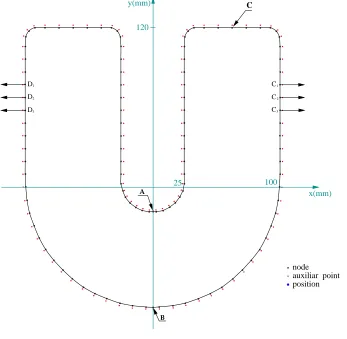
To illustrate the capability of the proposed approach to solve two-dimensional linear elastic problem, let us consider the problem and boundary conditions defined in the domain, depicted in figure (2). The material properties are2

6

4

, for elasticity modulus and3

, for Poisson’s coefficient. Furthermore, we assume as basis functions, first degree polynomials and evaluate the unknown functions , ,

M

and

P at boundary using Eq. (37). To this point, it is important to mention that

the auxiliary points are positioned outside the domain, apart from the nodes at boundary, a distance of 20% the length of the discretization step. This procedure allow us to avoid the singularity in the integral evaluated at boundary. In order to show the numerical convergence of the proposed approach we report numerical results for the following averaged distances between nodes 4

, and 6

mm and we compare the results with the ones attained by the finite element method (ABAQUS version

5.8.1). For the finite element results we take advantage of the problem symmetry. However, symmetry can not be considered in our approach because the nodes at the corner of the domain. Numerical comparisons for the maximum and minimum values for and (

) as well the values of the stress MYM

PP

and

M

P

, the values of stress MYM

at points and

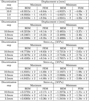
(see figure (2)) and the values of displacements and at point (see figure (2)) are reported in tables (1) to (3). From the previous results

we readily notice the numerical convergence of the results encountered by this method and the good comparison with the ones achieved by the finite elements method, when we refine the mesh size of the discretized domain. For sake of completeness in figure (3) we report the results for stress distribution in direction by discussed methods for the mesh size of

6

. Given a

closer look in these results we promptly observe a very good agreement.

Now, let us assume assume that the considered problem has unique solution. Furthermore, we have previously shown that the achieved integral formulation for the solution, through the Fourier Transform technique, is the solution of the problem under consideration. Therefore, we are confident to affirm that the results encountered, actually are solutions of the problem discussed. This argument is reinforced by the good coincidence with finite elements results.

(6)

Table 1: Maximum and minimum for the displacement and and for the stress MM

, P!P

and

M

P

.

Discretization Displacement

step Maximum Minimum

BEM FEM BEM FEM

!""#%$ !&"%$

' "$ "# !$#%$ !&#"%$

$' ( !%$ !&"%$

Discretization Displacement)

BEM FEM BEM FEM

'

"$'*$ +,%$ -'" -"# (

#*$ "$%$ -'""" -"" $(

""*$ "%$ -'""" -""

Discretization Stress.0//

21435&

BEM FEM BEM FEM

'

##"$!$ "6 $ $(#$'$! $ $'"6 $ (

#!$ "6 $ $(#""! $ $'#"6 $ $(

$!$ 6 $ $(##! $ $'#"6 $

Discretization Stress.0787

21435&

BEM FEM BEM FEM

'

&"8!$ &"6 $ $(98$#! $ :""6 $ (

&(!$ &"6 $ $(""! $ $'"6 $ $(

&($'8!$ &"6 $ $(! $ $'"6 $

Discretization Stress.0/ 7

21435&

BEM FEM BEM FEM

'

#"$"$!$ :$'+#6 $ :$$"#"! $ :"$(6 $ (

(!$ +,6 $ :$""! $ :"$6 $ $(

""!$ "6 $ :$&8"! $ :"$6 $

Table 2: Stress MYM

at positions d

6

and d

4

.

Location Discretization . //

21;35<

x y step BEM FEM

8

'##"$"! $ "$"#=>$ '

$"(

(

'#"! $ "$"=>$ $(

'"$! $ ""=>$ 8

$(#$(! $ $'"=>$ '

:

(

$(###! $ $'#$"#=>$ $(

$(#"$(! $ $'#""=>$

Table 3: Displacements and at positions @?

6

4

6

.

Location Discretization

)

x y step BEM FEM BEM FEM

$ ' :"( :"""$ $'

$'

'

" '"" :"" :"8" $'

(7)

C

!"

#$

%&

'(

)*

+,

--.

//0

112 334 556 778

99: ;;< ==>

??@

AAB CD EF GH IJ KL MNOO

PPQQRR ST

UV

WX

YYZ [[\

]^

__ ``

ab

cd

ef

gg hh

ij

kkl

mm nn

op

qq rr

st

uuv

wx

yz

{|

}~

¡¡¢

£¤

¥¦

§¨

©ª

«¬

®

¯°

±²

³´

µ¶

·¸

¹¹

ºº »»¼¼

½½¾¿À

ÁÂ

ÃÃ ÄÄ ÅÅ

ÆÆ ÇÈ

ÉÉ ÊÊ

ËËÌ ÍÎ ÏÏÐ ÑÒ

ÓÔ

ÕÖ

×Ø ÙÚ

ÛÜ

ÝÞ

ßà

ááâ

120

25 100

B A

C

2

3 1

D

3

D D

2

1

C

node auxiliar point position

y(mm)

x(mm)

Figure 2: Discretized domain.

Boundary conditions at nodes: ãåäçæéèëêíìïîíðñèòêôó, õöäçæ÷èòêíìùøúèëêûó, üþýïÿ ÿ äîúè ê ê ì î ð èëêûó, ý ÿ ÿ äî è

(8)

(a) BEM.

X Y

Z

8.54+01

-2.76+01

8.54+01

7.79+01 7.03+01

6.28+01 5.53+01 4.77+01

4.02+01 3.27+01

2.51+01 1.76+01

1.01+01 2.53+00

-5.00+00 -1.25+01 -2.01+01

-2.76+01 default_Fringe : Max 8.54+01 @Nd 1584 Min -2.76+01 @Nd 1520 MSC/PATRAN Version 9.0 28-Jun-00 19:16:46

Fringe: Static, Step1,TotalTime=1.: Stress, Components-(NON-LAYERED) (XX)

X Y

Z

(b) FEM.

Figure 3: Color map for stress distribution MM

(color scales

4

) obtained for6

size step.

ACKNOWLEDGMENT

The second author is indebted to CNPq/Brazil (Conselho Nacional de Desenvolvimento Científico e Tecnológico) for partial financial support of this work.

REFERENCES

1. G. G. Furtado, M. T. de Vilhena, and T. R. Strohaecker, “An approach to boundary integral elment via fourier transforms”, Eng. Anal. Bound. Elem., 22(3):215-220, 1998.