Source Apportionment of PM2.5 using Three-Dimensional Air Quality Models: Analysis and Inter-Comparison of Two Source Apportionment Methods.

ABSTRACT

BURR, MICHAEL J. Source Apportionment of PM2.5 using Three-Dimensional Air Quality Models: Analysis and Inter-Comparison of Two Source Apportionment Methods. (Under the direction of Dr. Yang Zhang).

Source apportionment is a vital first step in creating the most effective reduction

strategies in non-attainment areas. Receptor-based models that utilize observational data

have been the traditionally-used source apportionment methods. More recent studies have

made use of 3-dimensional air quality models to conduct source apportionment. These

source-oriented methods have the potential to provide a much more robust source

apportionment dataset, both spatially and temporally. This research evaluates two

source-oriented source apportionment methods, the Particle Source Apportionment Technology

(PSAT) and the Brute-Force direct sensitivity analysis Method (BFM). PSAT is

implemented in the Comprehensive Air Quality Model with extensions (CAMx) while the

Community Multiscale Air Quality (CMAQ) modeling system is utilized to conduct source

apportionment via the BFM. Source apportionment is conducted for 10 source categories

(i.e., biogenic, biomass burning, coal combustion, diesel vehicles, gasoline vehicles,

industrial processes, miscellaneous area sources, other combustion, other mobile sources, and

waste disposal and treatment ) over the eastern U.S. at a horizontal grid spacing of 12-km for

both January and July of 2002 using both BFM and PSAT.

In the baseline simulation, O3 and PM2.5 are overpredicted by both models in January

and underpredicted by both models in July, with CAMx generally predicting higher values

than CMAQ in both months. When compared to satellite data, CMAQ shows good

underpredicts all column variables, with the largest bias occurring for AOD. In January,

CMAQ gives biomass burning as the most important source of PM2.5, with a contribution of

13.7% to domain-wide monthly-mean PM2.5. Miscellaneous area sources and coal

combustion are the next two largest contributors to domain-wide PM2.5 from the BFM, with

contributions of 11.8% and 10.8%, respectively. PSAT, however, gives different rankings in

terms of the most important sources of PM2.5 in January. PSAT identifies coal combustion as

the most important source in January, with a monthly-mean percentage contribution of 14.0%

to domain-wide PM2.5. The next two largest sources from PSAT are biomass burning and

other mobile sources, with contributions of 11.3% and 6.8%, respectively. The two methods

are in agreement that coal combustion is the most important source of PM2.5 in July, with

contributions of 30.8% and 21.0% to domain-wide PM2.5 from BFM and PSAT, respectively.

The BFM and PSAT also agree on miscellaneous area sources being the next largest source

in July, with contributions of 8.9% and 8.1%, respectively. The next most important source

from both the BFM and PSAT is industrial processes, with monthly-mean percentage

contributions of 6.9 and 6.2%, respectively.

While PSAT is found to be more computationally efficient than BFM and also has the

ability to account for 100% of the baseline PM2.5, BFM can better able capture the indirect

effects that result from interactions between secondary PM species and their gaseous

precursors. However, BFM is also subject to limitations, including its relative computational

inefficiency and its assumption that the emissions of all the source categories are linear and

additive. It is found that for primary PM species whose concentrations are linearly related to

emissions, BFM and PSAT are equivalent. However, the two methods differ significantly for

concentrations and lower concentrations of radical species. It is important to exercise caution

when using each of these tools while being mindful of the strengths and weaknesses of each

Source Apportionment of PM2.5 Using Three-Dimensional Air Quality Models: Analysis and Intercomparison of Two Source Apportionment Methods

by Michael J. Burr

A thesis submitted to the Graduate Faculty of North Carolina State University

in partial fulfillment of the requirements for the degree of

Master of Science

Atmospheric Sciences

Raleigh, North Carolina

2010

APPROVED BY:

_____________________________ ___________________________

Dr. Christopher Frey Dr. Viney Aneja

_________________________________ Dr. Yang Zhang

ii

BIOGRAPHY

Michael Burr was born and raised in Perry, OH where his interest in meteorology

began as a childhood fear of thunderstorms. He graduated from Perry High School in 2003

upon which he entered Ohio University to pursue a Bachelor‟s degree in meteorology. During his undergraduate studies, he was an active member of the Ohio University‟s

meteorology club. During his first three years at Ohio University, he was a staff forecaster

for the Scalia Lab for Atmospheric Analysis where he provided detailed daily 5-day weather

forecasts for resident of Southeast Ohio. In the spring of 2007, he was awarded the

Voinovich scholarship for outstanding students and began funded research with the Ohio University‟s Center for Air Quality. As an undergraduate research assistant, he provided

daily fine particulate matter forecasts for Northeast Ohio. In addition to forecasting PM2.5, he assisted in daily maintenance of the Center‟s air quality monitoring station while assisting in

researching the effects of wet deposition of mercury throughout the Ohio River Valley. This

research experience shifted his interests from operational forecasting to air quality. He

graduated from Ohio University in June 2008 with a Bachelor of Science degree in

meteorology with minors in physics and mathematics. He was accepted to North Carolina State University‟s Marine, Earth, and Atmospheric Science Graduate Program in March 2008

and began working in Dr. Yang Zhang‟s Air Quality Forecasting Laboratory in August 2008.

Before he began working with Dr. Zhang, he served as an intern during the summer of 2008

at the U.S. EPA National Center for Environmental Assessment. He also worked as an intern

iii

ACKNOWLEDGEMENTS

I would first like to thank my committee members, Drs. Yang Zhang, Christopher

Frey, and Viney Aneja. I would like to extend further gratitude to Dr. Zhang for giving me

the opportunity to further my studies at North Carolina State University while conducting

this research. She gave me endless support and guidance while providing me with numerous

opportunities to advance my scientific knowledge and experience throughout my graduate

studies, all of which I am extremely grateful for. I would also like to thank my

undergraduate professors (Dr. Ronald Isaac, Christopher Towe) in the meteorology

department at Ohio University as well as my advisors at the Ohio University Center for Air

Quality (Dr. Kevin Crist, Gary Conley, Myoungwoo Kim) for providing me with the

knowledge base required to further my education through my graduate studies.

I would like to acknowledge and thank the U.S. EPA for funding this project through

the Science to Achieve Results grant # R833863 and the USDA National Research Initiative

Competitive grant # 2008-35112-18578. Thanks are also due to numerous people who have

contributed to this research in one way or another: Dennis McNally, Cyndi Loomis, and

regory Stella, Alpine Geophysics, Inc; Pat Brewer, Michael Abraczinksas, George Bridgers,

Bebhinn Do, and Chris Misenis, North Carolina Department of Environmental and Natural

Resources; and Gary Wilson, Ralph Morris, and Greg Yarwood, ENVIRON, Inc.

I wish to extend special gratitude to all the members of the Air Quality Forecasting

Lab, past and present. Each has provided endless guidance and assistance throughout my

iv

hard work in the lab. Extra thanks go to Kristen Olsen, who took extra time and went far

beyond what was required in helping me with my research. Lastly, to my family: my mom,

dad, and sisters, thank you for everything. It is with your love and support throughout my

entire life that I am able to be where I am today. And to Renee, your love, encouragement,

support, and most importantly your patience throughout this long and challenging experience

v

TABLE OF CONTENTS

LIST OF TABLES... viii

LIST OF FIGURES... xi

LIST OF ACRONYMS... xx

1 CHAPTER 1. INTRODUCTION... 1

1.1 Background and Motivation... ₁

1.2 Impacts of PM2.5... ₁

1.3 _{State Implementation Plans... 2}

1.4 Objectives... ₄

2 CHAPTER 2. LITERATURE REVIEW... 5

2.1 Theoretical Basis of Source Apportionment Methods... 7

2.1.1 Receptor Based Methods... 7

2.1.1.1 Chemical Mass Balance... 7

2.1.1.2 Positive Matrix Factorization... ₉

2.1.2 Source-Oriented Methods... 10

2.1.2.1 Sensitivity Analysis Methods... 11

2.1.2.1.1 The Brute-Force Method (BFM)... 11

2.1.2.1.2 The Decoupled Direct Method (DDM)... 12

2.1.2.2 Reactive Tracers Method... 13

2.1.2.2.1 The Particulate Source Apportionment Technology (PSAT)... 13

2.1.2.2.2 Tagged Species Within CMAQ... 16

2.1.2.2.3 Comparisons of Source Apportionment and Source Sensitivity... 17

2.2 Current Status and Major Challenges of Source Apportionment Studies... 25

2.2.1 Major Sources of Fine Particulate Matter over the Eastern U.S... 25

vi

3 CHAPTER 3. SOURCE APPORTIONMENT METHODOLOGIES AND

BASELINE SIMULATIONS... 31

3.1 Modeling System... 31

3.1.1 MM5... 31

3.1.2 SMOKE... 34

3.1.3 CMAQ/BFM... 34

3.1.4 CAMx/PSAT... 35

3.2 Episode Description... 35

3.3 Evaluation of Baseline Simulations... 38

3.3.1 Observational Datasets... 38

3.3.2 Evaluation Protocol... 39

3.3.3 Surface Evaluation of O3 and PM2.5... 41

3.3.4 Spatial Distribution of O3 and PM2.5... 63

3.3.5 Wet Deposition Fluxes... 64

3.3.6 Column Variables... 67

3.4 Summary... 76

4 CHAPTER 4. SOURCE APPORTIONMENT SIMULATIONS USING CMAQ... 78

4.1 Source Selection and Analysis Method... 78

4.2 Source Apportionment Results using CMAQ/BFM... 80

4.2.1 Domain-Wide Analysis... 80 4.2.2 Spatial Distribution of Emissions and Source Contributions... 88

4.3 Site Specific Analysis... 138

4.4 Summary... 150

vii

5.1 Simulation Setup... 152

5.2 Source Apportionment Results and Intercomparison with CMAQ/BFM... 152

5.3 Spatial Distribution of CAMx/PSAT Source Contributions... 155

5.4 Site Specific Analysis... 192

5.5 _{Comparison of Computational Speeds of BFM and PSAT... 219}

5.6 Implications of Source Apportionment to the State Implementation Plan (SIP) and Human-Health Based Epidemiological Studies... 219

6 _{CHAPTER 6. CONCLUSIONS AND RECOMMENDATIONS... 224}

viii

LIST OF TABLES

Table Page

Table 2.1 Summary of existing source apportionment methods...

6

Table 2.2 Contributions of major sources of PM2.5 as resolved by previous studies in the southeastern U.S. in the winter months (expressed in percentage)……

19

Table 2.3 Contributions of major sources of PM2.5 as resolved by previous studies in the southeastern U.S. in the spring months (expressed in percentage)... ₂₀

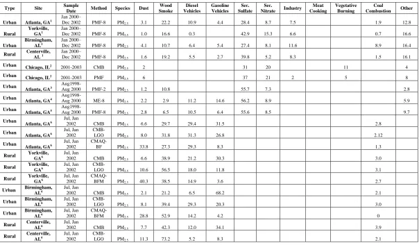
Table 2.4 Contributions of major sources of PM2.5 as resolved by previous studies in the southeastern U.S. in the summer months (expressed in percentage)...

21

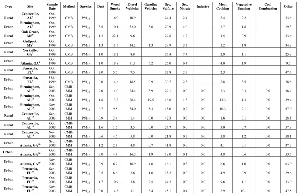
Table 2.5 Contributions of major sources of PM2.5 as resolved by previous studies in the southeastern U.S. in the autumn months (expressed in percentage)...

22

Table 2.6 Contributions of major sources of PM2.5 as resolved by previous studies in the southeastern U.S. (multi-month, expressed in percentage)...

23

Table 3.1 MM5 Model Configurations... 33

Table 3.2 CMAQ and CAMx configurations used in this research... 36

Table 3.3 The observational networks and satellites used in model evaluation, as well as the variables evaluated, the sampling frequency, and the number of sites within the 12-km domain...

40

Table 3.4 Performance statistics for O3 in January 2002... 42

ix

Table 3.6 Performance statistics for monthly-mean BCin January 2002... 44

Table 3.7 Performance statistics for monthly-mean OCin January 2002... 45

Table 3.8 Performance statistics for monthly-mean TCin January 2002... 46

Table 3.9 Performance statistics for monthly-mean NO3- in January 2002... 47

Table 3.10 Performance statistics for monthly-mean SO42- in January 2002……... 48

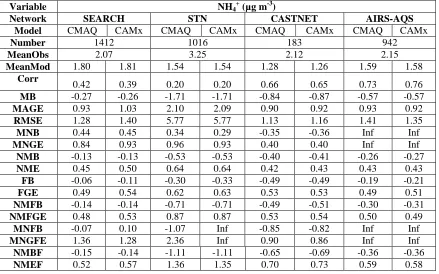
Table 3.11 Performance statistics for monthly-mean NH4+ in January 2002………... 49

Table 3.12 Performance Statistics for O3 in July 2002... 50

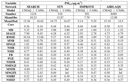
Table 3.13 Performance statistics for monthly-mean PM2.5 in July 2002... 51

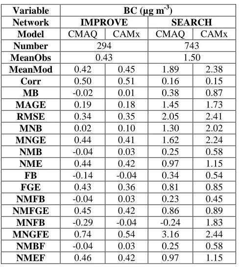
Table 3.14 Performance statistics for monthly-mean BC in July 2002... 52

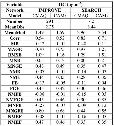
Table 3.15 Performance statistics for monthly-mean OC in July 2002... 53

Table 3.16 Performance statistics for monthly-mean TC in July 2002... 54

Table 3.17 Performance statistics for monthly-mean NO3- in July 2002... 55

Table 3.18 Performance statistics for monthly-mean SO42- in July 2002... 56

Table 3.19 Performance statistics for monthly-mean NH4+ in July 2002………... 57

Table 3.20 Performance statistics for wet deposition in January 2002...

65

x

Table 3.22 Performance statistics for satellite-derived variables in January 2002 (simulated values are from CMAQ)...

68

Table 3.23 Performance statistics for satellite derived variables in July 2002 (simulated values are from CMAQ)...

69

Table 4.1 Source categories analyzed in this study... 79

Table 4.2 Monthly-mean percentage contributions of each source category to speciated emissions in January...

82

Table 4.3 Monthly-mean percentage contributions of each source category to speciated emissions in July...

82

Table 4.4 Domain-wide monthly-mean percentage contributions to PM2.5 in January from BFM...

83

Table 4.5 Domain-wide monthly-mean percentage contributions to PM2.5 in July from BFM...

83

Table 4.6 Monthly-mean percentage contributions to PM2.5 at representative sites in July (top 3 sources in red, bottom 3 in green)...

136

Table 4.7 Monthly-mean percentage contributions to PM2.5 at representative sites in July (top 3 sources in red, bottom 3 in green)...

137

Table 5.1 Domain-wide monthly-mean percent contributions to PM2.5 in January from PSAT...

154

Table 5.2 Domain-wide monthly-mean percent contributions to PM2.5 in July from PSAT...

154

xi

LIST OF FIGURES

Figure Page

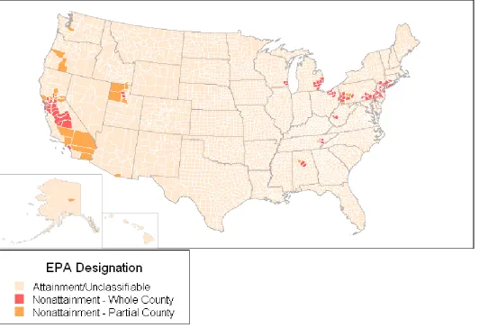
Figure 1.1 U.S. EPA area designations for 2006 24-hour fine particle (PM2.5) standards (http://www.epa.gov/pmdesignations/index.htm)...

3

Figure 3.1

The domain used in this research: 12-km horizontal grid spacing over the

eastern U.S………. 32

Figure 3.2 Wet deposition of SO42- from CMAQ (left) and CAMx (right) in

January………... ₅₈

Figure 3.3 Spatial distribution monthly mean maximum 8-hour average O3 concentrations simulated by CMAQ (left) and CAMx (right) overlaid with observations from AIRS-AQS, CASTNET, and SEARCH in January (top) and July (bottom)...

61

Figure 3.4 Spatial distribution monthly mean PM2.5 concentrations simulated by CMAQ (left) and CAMx (right) overlaid with observations from AIRS-AQS, IMPROVE, STN, and SEARCH in January (top) and July (bottom)...

62

Figure 3.5 Monthly-mean column CO from MOPITT (top) and CMAQ(bottom) for January (left) and July (right)...

70

Figure 3.6 Monthly-mean column NO2 from GOMES (top) and CMAQ(bottom) for January (left) and July (right)...

71

Figure 3.7 Monthly-mean column O3 from TOMS (top) and CMAQ(bottom) for January (left) and July (right)...

xii

Figure 3.8 Monthly-mean column AOD from MODIS (top) and CMAQ(bottom) for January (left) and July (right)...

73

Figure 4.1 Spatial distribution of monthly-mean percentage contributions of coal combustion emissions to baseline emissions in January (top) and July (bottom)...

89

Figure 4.2 Domain-wide monthly-mean contributions of coal combustion emissions to PM2.5 and its individual components in January... ₉₀

Figure 4.3 Domain-wide monthly-mean contributions of coal combustion emissions to PM2.5 and its individual components in the first 6 layers in January………...

91

Figure 4.4 Domain-wide monthly-mean contributions of coal combustion emissions to PM2.5 and its individual components in July... ₉₂

Figure 4.5 Domain-wide monthly-mean contributions of coal combustion emissions to PM2.5 and its individual components in the first 6 layers in July...

93

Figure 4.6 Spatial distribution of monthly-mean percentage contributions of diesel vehicle emissions to baseline emissions in January (top) and July (bottom)...

94

Figure 4.7 Domain-wide monthly-mean contributions of diesel vehicle emissions to PM2.5 and its individual components in January... ₉₅

Figure 4.8 Domain-wide monthly-mean contributions of diesel vehicle emissions to PM2.5 and its individual components in July... ₉₆

xiii

Figure 4.10 Domain-wide monthly-mean contributions of biomass burning emissions to PM2.5 and its individual components in January... ₉₈

Figure 4.11 Domain-wide monthly-mean contributions of biomass burning emissions to PM2.5 and its individual components in July... ₉₉

Figure 4.12 Spatial distribution of monthly-mean percentage contributions of gasoline vehicle emissions to baseline emissions in January (top) and July (bottom)...

100

Figure 4.13 Domain-wide monthly-mean contributions of gasoline vehicle emissions to PM2.5 and its individual components in January... ₁₀₁

Figure 4.14 Domain-wide monthly-mean contributions of gasoline vehicle emissions to PM2.5 and its individual components in July... ₁₀₂

Figure 4.15 Spatial distribution of monthly-mean percentage contributions of industrial processes emissions to baseline emissions in January (top) and July (bottom)... ₁₀₃

Figure 4.16 Domain-wide monthly-mean contributions of industrial processes emissions to PM2.5 and its individual components in January... ₁₀₄

Figure 4.17 Domain-wide monthly-mean contributions of industrial processes emissions to PM2.5 and its individual components in July... ₁₀₅

Figure 4.18 Spatial distribution of monthly-mean percentage contributions of waste disposal and treatment emissions to baseline emissions in January (top) and July (bottom)...

106

xiv

Figure 4.20 Domain-wide monthly-mean contributions of waste disposal emissions to PM2.5 and its individual components in July………. ₁₀₈

Figure 4.21 Spatial distribution of monthly-mean percentage contributions of biogenic emissions to baseline emissions in January (top) and July

(bottom)………. ₁₀₉

Figure 4.22 Domain-wide monthly-mean contributions of biogenic emissions to PM2.5 and its individual components in January... ₁₁₀

Figure 4.23 Domain-wide monthly-mean contributions of biogenic emissions to PM2.5 and its individual components in July... ₁₁₁

Figure 4.24 Spatial distribution of monthly-mean percentage contributions of other combustion emissions to baseline emissions in January (top) and July (bottom)...

112

Figure 4.25 Domain-wide monthly-mean contributions of other combustion emissions to PM2.5 and its individual components in January... ₁₁₃

Figure 4.26 Domain-wide monthly-mean contributions of other combustion emissions to PM2.5 and its individual components in July... ₁₁₄

Figure 4.27 Spatial distribution of monthly-mean percentage contributions of other mobile source emissions to baseline emissions in January (top) and July (bottom)...

115

Figure 4.28 Domain-wide monthly-mean contributions of other mobile source emissions to PM2.5 and its individual components in January... ₁₁₆

xv

Figure 4.30 Spatial distribution of monthly-mean percentage contributions of miscellaneous area sources emissions to baseline emissions in January (top) and July (bottom)………..

118

Figure 4.31 Domain-wide monthly-mean contributions of miscellaneous area source emissions to PM2.5 and its individual components in January... ₁₁₉

Figure 4.32 Domain-wide monthly-mean contributions of miscellaneous area source emissions to PM2.5 and its individual components in July... ₁₂₀

Figure 4.33 Monthly-mean baseline NH3 emissions in January (left) and July

(right)………. ₁₂₂

Figure 4.34 Monthly mean PBL Height in January (left) and July (right) as well as monthly-mean daytime (8am – 7pm) and nighttime (8pm – 7am) PBL heights in January and July...

126

Figure 4.35 Monthly-mean contribution (in ppb) of miscellaneous areas sources to HNO3 in January (left) and July (right) (Note that negative numbers indicate an increase of HNO3 when miscellaneous area source emissions are eliminated)...

133

Figure 4.36 Monthly-mean percentage contributions to PM2.5 at urban, rural, remote, and coastal sites in January (top) and July (bottom)...

140

Figure 4.37 Comparison of SA results with other studies at JST in January (top) and July (bottom)...

141

Figure 4.38 Comparison of SA results with other studies at CTR in January (top) and July (bottom)...

142

Figure 4.39 Temporal variations of source contributions at JST in January (top) and July (bottom)...

xvi

Figure 4.40

Weekend effect for each source category in January (top) and

July (bottom)... 147

Figure 5.1 Domain-wide monthly-mean contributions of coal combustion emissions to PM2.5 and its individual components in January... ₁₅₆

Figure 5.2 Domain-wide monthly-mean contributions of coal combustion emissions to PM2.5 and its individual components in July... ₁₅₇

Figure 5.3 Domain-wide monthly-mean contributions of diesel vehicle emissions to PM2.5 and its individual components in January... ₁₅₈

Figure 5.4 Domain-wide monthly-mean contributions of diesel vehicle emissions to PM2.5 and its individual components in July... ₁₅₉

Figure 5.5 Domain-wide monthly-mean contributions of biomass burning emissions to PM2.5 and its individual components in January... ₁₆₀

Figure 5.6 Domain-wide monthly-mean contributions of biomass burning emissions to PM2.5 and its individual components in July... ₁₆₁

Figure 5.7 Domain-wide monthly-mean contributions of gasoline vehicle emissions to PM2.5 and its individual components in January... ₁₆₂

Figure 5.8 Domain-wide monthly-mean contributions of gasoline vehicle emissions to PM2.5 and its individual components in July... ₁₆₃

Figure 5.9 Domain-wide monthly-mean contributions of industrial processes emissions to PM2.5 and its individual components in January... ₁₆₄

xvii

Figure 5.11 Domain-wide monthly-mean contributions of waste disposal and treatment emissions to PM2.5 and its individual components in January.. ₁₆₆

Figure 5.12 Domain-wide monthly-mean contributions of waste disposal and treatment emissions to PM2.5 and its individual components in July... ₁₆₇

Figure 5.13 Domain-wide monthly-mean contributions of biogenic emissions to PM2.5 and its individual components in January... ₁₆₈

Figure 5.14 Domain-wide monthly-mean contributions of biogenic emissions to PM2.5 and its individual components in July... ₁₆₉

Figure 5.15 Domain-wide monthly-mean contributions of other combustion emissions to PM2.5 and its individual components in January... ₁₇₀

Figure 5.16 Domain-wide monthly-mean contributions of other combustion emissions to PM2.5 and its individual components in July... ₁₇₁

Figure 5.17 Domain-wide monthly-mean contributions of other mobile source emissions to PM2.5 and its individual components in January... ₁₇₂

Figure 5.18 Domain-wide monthly-mean contributions of other mobile source emissions to PM2.5 and its individual components in July...

173

Figure 5.19 Domain-wide monthly-mean contributions of miscellaneous area source emissions to PM2.5 and its individual components in January... ₁₇₄

Figure 5.20 Domain-wide monthly-mean contributions of miscellaneous area source emissions to PM2.5 and its individual components in July... ₁₇₅

Figure 5.21 Monthly-mean PM2.5 contributions (µg m-3) from coal combustion from BFM (left) and PSAT (right) in January...

xviii

Figure 5.22 Wet deposition fluxes of PSO4 from CMAQ (left) and CAMx (right) in January and July and the monthly-mean absolute difference in PSO4 wet deposition (CAMx – CMAQ)...

178

Figure 5.23 Monthly-mean biogenic VOC emissions and baseline SOA concentrations from CMAQ and CAMx in January (top) and July (bottom)……….

185

Figure 5.24 Simulated baseline H2O2 concentrations (ppb) from CMAQ (left) and CAMx (right)...

188

Figure 5.25 Absolute difference in monthly-mean baseline O3 (ppb) between CAMx and CMAQ in July...

189

Figure 5.26 Monthly-mean simulated cloud fraction from MM5 in July 2002…….... 189

Figure 5.27 Monthly-mean PM2.5 contributions at Jefferson Street (Atlanta), GA (top) and Yorkville, GA (bottom) in January (left) and July (right) of 2002 from PSAT and BFM... ₁₉₃

Figure 5.28 Monthly-mean PM2.5 contributions at Birmingham, AL (top) and Centreville, AL (bottom) in January (left) and July (right) of 2002 from PSAT and BFM...

194

Figure 5.29 Monthly-mean PM2.5 contributions at Gulfport, MS (top) and Oak Grove, MS (bottom) in January (left) and July (right) of 2002 from PSAT and BFM...

195

Figure 5.30 Monthly-mean PM2.5 contributions at Pensacola, FL (top) and Outlying Landing, FL (bottom) in January (left) and July (right) of 2002 from PSAT and BFM...

xix

Figure 5.31 Monthly-mean PM2.5 contributions at Great Smoky Mountain National Park (top) and Charlotte, NC (bottom) in January (left) and July (right) of 2002 from PSAT and BFM………...

197

Figure 5.32 Monthly-mean PM2.5 contributions at Jamesville, NC (top) and Chicago, IL (bottom) in January (left) and July (right) of 2002 from PSAT and BFM...

198

Figure 5.33 Monthly-mean PM2.5 contributions at New York City, NY (top) and New Orleans, LA (bottom) in January (left) and July (right) of 2002 from PSAT and BFM... ₁₉₉

Figure 5.34 Monthly-mean PM2.5 contributions at Cincinnati, OH (top) and Knoxville, TN (bottom) in January (left) and July (right) of 2002 from PSAT and BFM...

200

Figure 5.35 Monthly-mean PM2.5 contributions at Norfolk, VA (top) and Nashville, TN (bottom) in January (left) and July (right) of 2002 from PSAT and BFM………...

201

Figure 5.36 Miscellaneous area source contributions to NO3- and NH4- from CMAQ and CAMx at JST (top left), YRK (top right), BHM (bottom left) and CTR (bottom right) in January...

209

Figure 5.37 Comparison of PSAT and BFM results at urban sites (top) and rural sites (bottom) in January (left) and July (right)... ₂₁₃

Figure 5.38 Comparison of PSAT and BFM results at remote sites (top) and coastal sites (bottom) in January (left) and July (right)...

xx

LIST OF ACRONYMS

3-D Three-Dimensional

AIRS-AQS Aerometric Information Retrieval System – Air Quality Subsystem

AOD Aerosol Optical Depth

AQM Air Quality Model

BC Black Carbon

BCON Boundary Conditions

BEIS Biogenic Emissions Inventory System

BFM Brute-Force Method

BHM Birmingham, Alabama

CAMx Comprehensive Air Quality Model with Extensions

CASTNET Clean Air Status and Trends Network

CB-IV Carbon Bond IV

CHI Chicago, Illinois

CIN Cincinnati, Ohio

CLT Charlotte, North Carolina

CMAQ Community Multiscale Air Quality modeling system

CMB Chemical Mass Balance

CO Carbon Monoxide

CTR Centreville, Alabama

xxi

DU Dobson Unit

EC Elemental Carbon

FB Fractional Bias

FDDA Four Dimensional Data Assimilation

FGE Fractional Gross Error

GOME Global Ozone Monitoring Experiment

GFP Gulfport, Mississippi

GRM Great Smoky Mountains National Park

H2O2 Hydrogen Peroxide

H2SO4 Sulfuric Acid

Hg Mercury

HNO3 Nitric Acid

IMPROVE Interagency Monitoring of Protected Visual Environments

IPCC International Panel on Climate Change

JMS Jamesville, North Carolina

JST Jefferson Street (Atlanta), Georgia

KNX Knoxville, TN

LGO Lipschitz Global Optimization

LRT Long Range Transport

M3DRY Models 3 Dry Deposition Module

MAGE Mean Absolute Gross Error

xxii

MCIP Meteorology-Chemistry Interface Processor

MM5 PSU/NCAR 5th generation Mesoscale Model

MNB Mean Normalized Bias

MNGE Mean Normalized Gross Error

MNGFE Mean Normalized Gross Fractional Error

MODIS Moderate Resolution Imaging Spectroradiometer

MOPITT Measurements of Pollutants in the Troposhpere

NAAQS National Ambient Air Quality Standards

NC North Carolina

NCAR National Center for Atmospheric Research

NCDENR North Carolina Department of Environmental and Natural Resources

NEI National Emissions Inventory

NEO New Orleans, Louisiana

NH3 Ammonia

NH4+ Ammonium

(NH4)2SO4 Ammonium Sulfate

NH4NO3 Ammonium Nitrate

NMB Normalized Mean Bias

NMBF Normalized Mean Bias Factor

NME Normalized Mean Error

NMEF Normalized Mean Error Factor

xxiii

NMFGE Normalized Mean Fractional Gross Error

NO Nitric Oxide

NO2 Nitrogen Dioxide

NO3- Nitrate

NOR Norfolk, Virginia

NOx Nitrogen Oxides

NYC New York City, New York

O3 Ozone

OAK Oak Grove, Mississippi

OC Organic Carbon

OIN Other Inorganics

OLF Outlying Landing, Florida

OM Organic Matter

OSAT Ozone Source Apportionment Technology

ORV Ohio River Valley

PA Process Analysis

PBL Planetary Boundary Layer

PM Particulate Matter

PMF Positive Matrix Factorization

PNS Pensacola, Florida

POA Primary Organic Aerosols

xxiv

PPTM Particle and Precursor Tagging Methodology

PSAT Particle Source Apportionment Technology

PSU Pennsylvania State University

RADM Regional Acid Deposition Model

RMSE Root Mean Square Error

RRTM Rapid Radiative Transfer Model

SA Source Apportionment

SEARCH Southeastern Aerosol Research and Characterization

SIP State Implementation Plan

SMOKE Sparse Matrix Operator Kernel Emissions

SO2 Sulfur Dioxide

SO42- Sulfate

SOA Secondary Organic Aerosol

SOAP Secondary Organic Aerosol Partitioning

SORGAM Secondary Organic Aerosol Model

STN Speciation Trends Network

TC Total Carbon

TOC Total Organic Compound

TOMS Total Ozone Mapping Spectrometer

TOR Thermal Optical Reflectance

TOT Thermal Optical Transmittance

xxv

U.S. United States

U.S. EPA U.S. Environmental Protection Agency

VISTAS Visibility Improvement State and Tribal Association of the Southeast

VOC Volatile Organic Compound

1

CHAPTER 1. INTRODUCTION

1.1 Background and Motivations

Particulate matter with an aerodynamic diameter of less than or equal to 2.5 microns

(PM2.5) is a well researched and documented pollutant due to its adverse health effects and

contributions to visibility degradation and climate change. In December 2006, the U.S.

Environmental Protection Agency (EPA) lowered the 24-hour National Ambient Air Quality

Standards (NAAQS) for PM2.5 from 60 to 35 µg m-3. In order to attain this standard, the 3-year

average of the 98th percentile of 24-hour average PM2.5 concentrations must not exceed 35 µg/m3

(http://www.epa.gov/air/criteria.html). In order to develop the most cost-effective reduction

strategies, it is essential to have an understanding of which sources are contributing to these

elevated PM2.5 concentrations. The research presented in this thesis work will focus on source

apportionment of PM2.5 using two commonly used three-dimensional air quality models (3-D

AQMS): the Models-3 Community Multiscale Air Quality (CMAQ) model (Byun and Ching, 1999; Binkowski and Roselle, 2003; Byun and Schere, 2006) and ENVIRON‟s Comprehensive

Air Quality Model with extensions (CAMx) (ENVIRON, 2006). The brute-force method (BFM)

is used within CMAQ along with the Particle Source Apportionment Technology (PSAT) within

CAMx in order to assess the impacts of 10 prescribed source categories on PM2.5 concentrations

over the eastern U.S.

1.1.1 Impacts of PM2.5

PM2.5 is of particular concern with respect to human health because they have the ability

2

can be trapped and potentially removed in the upper respiratory system (Brunekereef and

Holgate, 2002). Acute and chronic exposure to elevated levels of PM2.5 has been linked to

increased mortality rates, heart attacks, decreased lung function, increased asthma attacks, and

even premature death (Dockert et al., 1993; Ebelt et al., 2000; Laden et al., 2000; Peters et al.,

2001). PM2.5 also scatters and absorbs light in the atmosphere, thus altering the amount of solar radiation that reaches the Earth‟s surface. The International Panel on Climate Change‟s (IPCC)

2007 synthesis report (IPCC, 2007) stated that anthropogenic contributions to aerosol particles

produce a cooling effect with a total direct radiative forcing of -0.5 W/m2. In addition to the

direct effects, smaller particles can lead to more reflective clouds, thus increasing the albedo of the Earth‟s surface. The IPCC reported that this indirect cloud albedo forcing is on the order of

-0.7 W/m2. Additionally, particles can lead to visibility degradation by scattering and absorbing

light at wavelengths similar to the particle size. These fine particles are thus important in

degradation of visible light which have wavelengths of 0.4 to 0.7 µm.

1.1.2 State Implementation Plans

Because of the aforementioned adverse effects, the U.S. EPA has designated PM2.5 as one

of the six criteria pollutants regulated under the NAAQS. Any area that fails to meet these

standards based on ambient monitoring data is designated as a non-attainment area. Figure 1.1

shows the PM2.5 nonattainment areas designated by the EPA as of October, 2009. As the figure

shows, the most problematic regions in terms of particle pollution are the northeastern U.S. and

southern California. When an area is designated as nonattainment, the state where that

3

4

outlines a plan to achieve compliance within a nonattainment area. Failure to successfully

achieve this task can result in economic sanctions imposed by the federal government on that

state. In order for the state governments to develop the most effective reduction strategies,

there must be an understanding of which emission sources are contributing the greatest to

PM2.5.formation. The work in this thesis will contribute to a broad body of work in the

scientific community apportioning PM2.5 to potential emission sources that can be used as a

reference in formulation of the aforementioned reduction strategies

1.2 Objectives

The objectives of this research are to:

(1) conduct source apportionment of PM2.5 for 10 major source categories for

January and July 2002 using CMAQ with the brute force direct sensitivity

analysis method and the CAMx/PSAT reactive tracer method in order to

determine the major sources of PM2.5 over the eastern U.S.

(2) analyze predicted contributions from each source category for both methods

and discuss the relative importance of each source along with potential

implications for emission reduction strategies and component-based

epidemiological PM2.5 studies.

(3) compare and contrast simulated source contributions from each method, and

identify sources of major discrepancies in results obtained with both methods

5

CHAPTER 2. LITERATURE REVIEW

The determination of major sources of fine particulate matter in the United States has

become an increasingly important area of research, particularly over the past decade. Several

different methods of apportioning PM2.5 mass to probable emission sources exist, each with

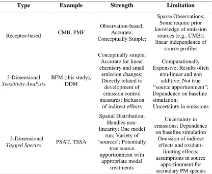
their own inherent strengths and limitations. Table 2.1 lists some of the major source

apportionment methods currently used along with their merits and limitations. Perhaps the

most widely-used source apportionment tools are receptor-oriented methods that aim to infer

contributions from different emission sources using measurements taken at a specific

receptor site. These methods have been well-documented in terms of their mathematical

formulation and development (Cooper and Watson, 1980; Waston, 1984; Hopke, 1991;

Henry, 1997; Watson et al., 2002; Hopke, 2003). More recent studies have implemented

3-dimensional air quality models (3-D AQMs) as a source-oriented method for apportioning

fine particle mass to potential sources. This thesis will compare two source apportionment

methods that utilize 3-D AQMs. An overview of the theoretical basis of two widely-used

receptor-oriented approaches as well as two classes of source-oriented methods for source

apportionment is given in section 2.1. Section 2.2 provides an overview of major sources of

fine particulate matter as resolved by other studies, with a particular emphasis on the sources

of PM2.5 over the eastern U.S. Also, the current status and major challenges with respect to

6

Table 2.1. Summary of existing source apportionment methods.

Type Example Strength Limitation

Receptor-based CMB, PMF

Observation-based; Accurate; Conceptually Simple;

Sparse Observations; Some require prior knowledge of emission

sources (e.g., CMB); linear independence of

source profiles

3-Dimensional

Sensitivity Analysis

BFM (this study), DDM

Conceptually simple; Accurate for linear chemistry and small

emission changes; Directly related to development of emission control measures; Inclusion

of indirect effects

Computationally Expensive; Results often

non-linear and non additive; Not true “source apportionment”; Dependence on baseline simulation;

Uncertainty in emissions

3-Dimensional

Tagged Species PSAT, TSSA

Spatial Distribution; Handles non-linearity; One model

run; Variety of „sources‟; Potentially true source apportionment with appropriate model treatments Uncertainty in emissions; Dependence

on baseline simulation Omission of indirect

effects and oxidant-limiting effects; assumptions in source

7

2.1 Theoretical Basis of Source Apportionment Methods

2.1.1 Receptor-Based Methods

Receptor-oriented source apportionment methods are widely-used tools throughout

the atmospheric science community that aim to resolve possible emission sources of a

particular PM2.5 sample based on its mass and chemical composition, which can then be

linked to the composition of possible emission sources. These receptor-based methods are

based on the conservation of mass of species, whose general form is given by:

1

,

ik kj ij

k

xij

g f

e

(2.1)

where xij is the ambient concentration of species j in sample i, fkj is the mass fraction of

species j in source k, gik is the source contribution of source k in sample i, and eij is the error

(Ke et al., 2008). Two of the most widely-used receptor models are positive matrix

factorization (PMF) and chemical mass balance (CMB), which will be discussed in the

following sections.

2.1.1.1Chemical Mass Balance

CMB uses a least-squares fitting method to minimize the difference between

measurements and modeled concentrations. CMB is a single sample receptor model to solve

equation 1, assuming that emission source profiles (fjk) are known. Similar to the object

8

2

2 2 2

1 1 1

2

[(

) / (

)]

jk

n N N

jk

ij xj f

j k k

x

f g

g

where xij is the ambient concentration of species j in sample i,fjk is the mass fraction of

species j in source k, gjkis the source contribution of source k in sample i, σxj is the

uncertainty of the ambient concentration of species j, and σfjk is the uncertainty in the fraction

of species j in the source profile k.

CMB is a powerful tool for solving the mass balance equation for source

apportionment, given that there is knowledge of all sources impacting a receptor. CMB has

been widely used and documented, making it widely available and fairly simple to

implement. CMB is also observation-based, and is thus generally believed to be accurate,

though sparse observational data can often limit the robustness of the dataset. However,

CMB models are based on assumptions (among others) that all sources with a potential for

significantly contributing to the receptor are included in the analysis, and also that the source

compositions are linearly independent of each other (U.S. EPA, 1998). This linear

independence of source profiles is one of the major assumptions that limit the ability of CMB

to accurately identify and apportion mass between sources that share relatively similar

profiles (Marmur et al., 2005). To help address this issue, Schauer et al. (1996) developed a

CMB receptor model based on the use of organic compounds as tracers. Organic markers

within CMB have been widely-used in PM2.5 source apportionment studies (Schauer et al.,

2000; Zheng et al., 2002; Robinson et al., 2006; Zheng et al., 2006; Ke et al., 2008). Marmur

9

particle ratios with the hypothesis that sources with fairly similar PM2.5 emissions may have

significantly different gaseous emissions. The extended CMB is useful in addressing the

problem of co-linearity between source profiles. In addition to issues with co-linearity, CMB

approaches do not typically account for species transformations from the source to the

receptor (Lee et al., 2009). CMB is also limited by the requirement of previous knowledge

of the composition of emission sources impacting a receptor site. Additionally, sparse

observations available for CMB analysis limit spatial coverage of source contributions that is

often desired, particularly in the case of exposure modeling.

2.1.1.2 Positive Matrix Factorization

PMF (Paatero, 1997) aims to iteratively solve the equation

1

ij ij ij ij ih hj

p

h

E

X

Y

X

G F

(2.3)

where G and F are the left and right factor matrices to be determined, and E is the difference

matrix between measurement Xij, and model, Yij (Rizzo and Scheff, 2007). The solution

provided by PMF minimizes an object function, Q (E), based on uncertainties for each

observation (Paatero, 1997; Polissar et al., 1998). This function is defined as (Kim et al.,

2004): 2 1 1

(

)

i j ij

E

Q E

(2.4)

With regards to equation (1), PMF is advantageous as it does not require prior

10

equation (2.1) (Maykut et al., 2003). Another major advantage of PMF is its ability to handle

missing and below detection limit data (Liu et al., 2005). However, because PMF does not

require prior knowledge of the composition of emission sources, a large number of samples

are required in order to resolve source factors (Lee et al., 2008). PMF is also limited by its

inability to link observed factors directly with actual sources due to the fact that PMF is

based on statistical patterns of correlations, rather than source profiles (Sarnat et al., 2008).

However, PMF has shown to be a valuable alternative to traditional receptor models, and has

been widely applied in source apportionment of PM2.5 (Kim et al., 2003; Kim et al., 2004;

Liu et al., 2005; Liu et al., 2006; Hwang et al., 2007; Jaeckels et al., 2007).

2.1.2 Source-Oriented Methods

A second group of source apportionment tools used is based on 3-D AQMs. These

emission-based models, as opposed to receptor-based models, use a processed emission

inventory as the starting point. The continuity equation, given as (Byun and Ching, 1999):

1 2

(

)

( /

( , ,..., , , )

( , )

i

i i i i n i

dc

Uc

D

c

R c c

c T t

S x t

dt

is then solved to simulate the fate and transport of pollutants. In equation (2.5), ci is the

concentration of species i, U is the wind velocity vector, Di is the molecular diffusivity of

species i, Ri is the rate of concentration change of species i by chemical reactions, Si(x,t) is

the source/sink of i at location x and time t, ρ is the air density, and n is the number of

11

the temporal variation in source impacts a specific receptor site, while emission-based

models may be more spatially representative. Two classes of source apportionment methods

using 3-D AQMs are discussed in the following sections.

2.1.2.1Sensitivity Analysis Methods

Sensitivity analysis methods measure the model output response to a change in input.

While these methods are a valuable tool for policy-makers in analyzing the effects of

emission reductions on the atmosphere, they will not provide true source apportionment if the

relationship between the model input and output is non linear (Yarwood et al., 2005), as is

often the case (Ansari and Pandis, 1998, 1999; Hakami et al., 2004; Cohan et al., 2005;

Dennis et al., 2008). Two widely-used sensitivity analysis methods within 3-D AQMs are

discussed in the following section.

2.1.2.1.1 The Brute-Force Method (BFM)

The brute-force method (BFM) is the most straight-forward sensitivity analysis

method, in which a baseline simulation is compared against a sensitivity simulation in which

emissions of a certain source category are eliminated. The difference in simulated PM2.5

between the baseline and sensitivity simulation can be attributed as the contribution of the

source to PM2.5 concentrations. A mathematical representation of this concept is:

,

i base sen i

S

C

C

,

100 *

pi

base

C

C

S

12

1 n

tot i

i

S

S

where Si is the absolute contribution of source i in the same unit as the concentration, Spi is

the percentage contribution of source i, Cbase is the PM2.5 concentration from the baseline

simulation, and Csen,i is the PM2.5 concentration from the sensitivity simulation in which the

emissions from source i are eliminated, and Stot is the total contribution from n number of

sources.

This method is simple and can be applied to any model, but is inefficient and

computationally expensive, as a complete model simulation is required for each source

category. This method is also rooted in the assumption that the emissions from all source

categories within the emission inventory are linear and additive; this assumption may not

hold in highly non-linear systems. However, BFM is advantageous in its ability to capture

the indirect effects that result from the interactions between secondary PM species due to

their thermodynamic relationships. Also, the smaller concentration changes between

simulations may be influenced more by numerical noise within the model than by the change

in emissions (Koo et al., 2009a).

2.1.2.1.2 The Decoupled Direct Method (DDM)

The decoupled direct method (DDM) (Dunker, 1981, 1984) is an efficient and accurate alternative to the BFM. In the DDM, the model‟s governing equations are

differentiated with respect to a particular sensitivity parameter. The resulting set of equations

13

advantage of DDM is that it decouples the sensitivity equations from the governing model

equations, thus enhancing computational efficiency (Koo et al., 2007). DDM has generally

been applied to calculate first-order sensitivities of gaseous species (Dunker et al., 2002a,

2002b). Its use has recently been extended to PM (Napelenok et al., 2006; Koo et al., 2007).

While DDM has been applied to solve higher order sensitivities for gaseous species (Hakami

et al., 2003, 2004; Cohan et al., 2005; Koo et al., 2008), its use for PM is currently limited to

first order sensitivities. Therefore, DDM is limited in its ability to represent higher order

sensitivities associated with the formation of secondary PM species. Yang et al. (1997)

developed a version of DDM known as DDM-3D that has been applied in 3-D AQMs

(Mendoza-Dominguez et al., 2000; Hakami et al., 2004). While DDM directly solves

sensitivity equations derived from the governing equations of the model while using the same

time steps as the chemistry routine, DDM-3D uses separate, less complex algorithms with

different time steps to solve the chemistry sensitivity equations (Koo et al., 2007, 2009a).

2.1.2.2 Reactive Tracers Method

More recent studies have implanted a reactive tracers (or tagged species) method for

source apportionment of PM2.5. These reactive tracers are extra species added to a 3-D AQM

that track contributions of pollutants from specific source categories. These tagged species

undergo the same processes (i.e., wet, dry deposition) within the model as the bulk chemical

species (Baker and Timin, 2008). For a pollutant with a total concentration of X with i

number of sources, a reactive tracer xi is assigned to each source such that the sum of the

reactive tracers will equal the total concentration of the species (X = ∑xi). The reactive

14

source apportionment (Yarwood et al., 2005). Two recently-developed tagged species source

apportionment methods implemented in two widely-used 3-D AQMs are described further in

the following sections.

2.1.2.2.1 The Particulate Source Apportionment Technology (PSAT)

The Particulate Source Apportionment Technology (PSAT) is a reactive tracers

algorithm that has been implemented in the Comprehensive Air Quality Model with

Extensions (CAMx) and is publicly available (Yarwood et al., 2004; Wagstrom et al., 2008).

PSAT calculates source apportionment using tagged species that undergo the same

atmospheric processes as the bulk chemical species within the main model, closely

resembling the methodology of the Ozone Source Apportionment Technology (OSAT)

(ENVIRON, 2009), also developed by ENVIRON. PSAT aims to conduct source

apportionment by solving the change in concentrations of the reactive tracers over each time

step. This is accomplished by solving for the production and destruction of the reactive

tracers due to different processes, as described in equations (2.9) and (2.10), respectively

(ENVIRON, 2009):

(

)

( )

i i

i

a

a t

t

a t

A

a

(

)

( )

i i

i

b

b t

t

b t

B

b

where ai is the reactive tracer for species A, biis the reactive tracer for species B, and t is the

15

PSAT is designed to apportion sulfate (SO42-), nitrate (NO3-), ammonium (NH4+),

mercury (Hg), secondary organic aerosol (SOA), and six primary PM species (e.g., elemental

carbon (EC), primary organic aerosol (POA), fine crustal particles, other fine particles,

coarse crustal particles, and other coarse particles. Yarwood et al. (2005) provide a complete

description of the reactive tracers added for each species for the source category of interest along with a detailed description of the algorithm‟s formulation. PSAT is an offline source

apportionment method that calculates source contributions with separate source

apportionment algorithms rather than by the host model routines (Baker and Timin, 2008).

PSAT is advantageous in that it is an efficient method in comparison to the sensitivity

methods, allowing for source apportionment for several different source categories in a single

model simulation. Additionally, it can handle the issues of non-linearity that often limit

sensitivity methods, and thus have the potential to provide true source apportionment.

However, a major challenge of PSAT is the development of a feasible manner to assign

concentration changes to the reactive tracers due to non-linear processes, as there is no

unique way to accomplish this. Additionally, because PSAT is designed to apportion each

PM species to its primary precursor, it is unable to capture the indirect effects and oxidant

limiting effects that result from interactions between secondary PM species and their gaseous

precursors. Wagstrom et al. (2008) developed an online particulate source apportionment

algorithm (OPSA) that was implemented into a 3-D aerosol chemical transport model

(PMCAMx) (Gaydos etal., 2007) and compared it with the offline PSAT implemented by

Yarwood et al. (2005). The offline PSAT algorithm uses the same equations as the on-line

16

of tracking the source specific species separately, the offline algorithm uses the

apportionment of the upwind grid cell to apportion each species after the transport

calculations (Wagstrom et al., 2008). Wagstrom et al. (2008) found that the offline version

of PSAT compared well to the more rigorous online algorithm and has the advantage of

being more computationally efficient and simpler to implement.

2.1.2.2.2 Tagged Species within CMAQ

Similar tagged species source apportionment algorithms have also been implemented

in CMAQ. The Particle and Precursor Tagging Methodology (PPTM) was initially

implemented into CMAQ with the capabilities of tagging sulfur, nitrogen, and mercury

(Myers et al., 2006; ICF International, 2007a, 2007b). Bhave et al. (2007) later implemented

tracking of primary organic and elemental carbon. The Tagged Species Source

Apportionment (TSSA) algorithm was subsequently developed and implemented into CMAQ

with the capability of tagging approximately 20 new species (Tonnesen et al., 2005; Wang et

al., 2009). Like PSAT, TSSA is advantageous in its efficiency and ability to handle

non-linearity. Wang et al. (2009) compared TSSA to PSAT and found that the two algorithms

produced similar results in terms of ranks of source contributions. They did, however, find

differences between the source apportionment results from the two algorithms that in many

cases can be attributed in large part to differences in underlying model formulation (e.g.

vertical advection scheme, vertical eddy diffusivity values) as opposed to differences in the

source apportionment methodologies. Baker and Timin (2008) also found that the two

17

2.1.2.2.3 Comparisons of Source Apportionment and Source Sensitivity

While comparisons of different sensitivity methods have been widely conducted

(Dunker et al., 2002a; Hakami et al., 2004; Cohan et al., 2005; Napelenok et al., 2006; Koo et

al., 2007), as well as a few attempts at comparing different source apportionment methods

(Baker and Timin, 2008; Wagstrom et al., 2008; Wang et al., 2009), there have been limited

studies comparing recent tagged species (or “source apportionment”) methods with source

sensitivity methods. Dunker et al. (2002b) compared source apportionment of ozone using

OSAT with first order DDM sensitivities in terms of emissions and initial and boundary

conditions. They found that OSAT and DDM agreed reasonably well on the most important

contributors to the highest ozone concentrations but disagreed on about 20% of the important

contributors. Zhang et al. (2005) also compared OSAT with DDM and Process Analysis

(PA). They found that the NOx versus VOC-sensitivity of ozone chemistry predicted by the

three probing tools was similar over most of the domain, except in a few areas where O3

formation was predicted to be VOC-sensitive by PA and DDM but NOx-limited by OSAT.

In terms of ranks of O3 contributors, they found that DDM and PSAT agreed well on the sets

of top 10 O3 contributors, but predicted different rankings among those sets of top 10

contributors to the highest 1- and 8- hour average O3 concentrations.

Baek et al. (2005) compared the brute force method with a tagged species algorithm

in CMAQ (CMAQ-TR) for predicted contributions of 5 source categories to primary organic

aerosols (POA). They found that predicted contributions to POA of the 5 source categories

agreed well between the two methods, as is expected due to the linear relationship between

18

comparisons of source apportionment and source sensitivity for PM. They compared PSAT

and DDM to brute-force predicted contributions of point source SO2 emissions, on-road

mobile source emissions, and anthropogenic NH3 and NOx emissions to PM2.5 contributions

within CAMx. PSAT and DDM were compared to the brute-force method for various

emission reductions of 20 and 100%. They found that PSAT agreed well with the brute-force

method in situations where the emissions-concentration relationship was linear (e.g., primary

aerosols). They also found that PSAT agreed well with the brute-force method in situations

where the emission-concentration relationship was highly non-linear but there were no

indirect effects. PSAT and BFM disagreed in situations where the emission-concentration

relationship is highly non-linear and there are significant indirect effects and oxidant-limiting

effects. For example, contributions of PSAT to sulfate formation near a large point source

of SO2 were found to be smaller than the brute-force predicted contributions. This is due to

more availability of oxidants when an emission source is completely removed (as is the case

for BFM); PSAT does not take this indirect effect into account (Koo et al., 2009b). This is

19

Table 2.2. Contributions of major sources of PM2.5 from previous studies in the southeastern U.S. in the winter months (expressed in percentage).

Type Site Sample

Date Method Species Dust Wood Smoke Diesel Vehicles Gasoline Vehicles Sec. Sulfate Sec.

Nitrate Industry

Meat Cooking

Vegetative Burning

Coal

Combustion Other Urban Atlanta,

GA8

Jan.

2002 PMF-1 PM2.5 2.0 31.9 9.6 11.6 16.0 17.3 3.0 1.7 6.9 Urban Atlanta,

GA8

Jan.

2002 PMF-2 PM2.5 1.2 23.8 19.5 15.2 7.0 3.2 4.9 Rural Centreville,

AL9

Jan.

2000 CMB PM2.5 1.4 19.3 10.1 3.4 23.8 10.9 5.1 0.8 24.8 Urban Birmingham

, AL9

Jan.

2000 CMB PM2.5 2.5 27.4 24.1 4.1 17.1 12.1 2.8 1.4 7.3

Rural Oak Grove, MS9

Jan.

2000 CMB PM2.5 3.4 32.5 12.8 28.6 8.0 5.0 1.6 8.4

Urban Gulfport, MS9

Jan.

2000 CMB PM2.5 19.7 17.0 20.7 5.1 2.3 2.1 33.9

Rural Yorkville, GA9

Jan.

2000 CMB PM2.5 23.1 13.5 29.8 14.7 5.6 3.8 12.0 Urban Atlanta, _GA9

Jan.

2000 CMB PM2.5 31.3 23.2 7.1 17.4 11.5 2.6 4.2 8.1 Rural Pensacola,

FL9

Jan.

2000 CMB PM2.5 19.5 19.4 23.5 5.0 3.8 11.4 23.1 Urban Pensacola,

FL9

Jan.

2000 CMB PM2.5 3.7 64.2 22.6 5.0 24.3 5.6 4.7 6.4 Urban Birmingham

, AL10

Dec. 2003

CMB-MM PM2.5 0.0 23.3 15.7 18.2 24.5 1.9 0.0 6.4 3.2 0.0 21.9 Urban Birmingham

, AL10

Jan. 2004

CMB-MM PM2.5 0.8 9.0 25.0 8.9 13.5 4.8 0.0 4.7 0.5 0.0 59.5 Rural Centreville,

AL10

Dec. 2003

CMB-MM PM2.5 2.4 5.8 6.6 1.0 34.6 0.6 0.0 3.8 1.0 0.0 47.8 Rural Centreville,

AL10

Jan. 2004

CMB-MM PM2.5 0.1 30.4 1.8 1.4 16.2 1.7 0.0 2.5 3.9 0.0 41.6 Urban Atlanta,

GA10

Dec. 2003

CMB-MM PM2.5 1.1 9.6 12.7 3.4 32.5 0.8 0.0 3.2 1.1 0.0 49.7 Urban Atlanta,

GA10

Jan. 2004

CMB-MM PM2.5 0.8 27.7 9.3 12.8 13.9 5.3 0.0 7.6 3.8 0.0 41.7 Urban Pensacola,

FL10

Dec. 2003

CMB-MM PM2.5 0.3 21.3 4.0 3.4 23.5 0.5 0.0 9.1 9.6 0.0 39.5 Urban Pensacola,

FL10

Jan. 2004

CMB-MM PM2.5 0.1 21.2 7.1 5.2 17.2 1.0 0.0 5.4 14.7 0.0 38.1

Urban Atlanta, GA15

Jan. 2002

20

Table 2.3. Contributions of major sources of PM2.5 from previous studies in the southeastern U.S. in the spring months (expressed in percentage).

Type Site Sample

Date Method Species Dust Wood Smoke Diesel Vehicles Gasoline Vehicles Sec. Sulfate Sec.

Nitrate Industry

Meat Cooking

Vegetative Burning

Coal

Combustion Other

Rural

Centreville, AL9

Apr.

1999 CMB PM2.5 4.3 9.7 12.2 3.6 38.0 2.1 6.3 1.4 22.1 Urban

Birmingha m, AL9

Apr.

1999 CMB PM2.5 2.9 16.3 25 5.8 29.6 4.0 2.4 1.4 11.4 Rural

Oak Grove, MS9

Apr.

1999 CMB PM2.5 2.6 20.7 11.4 37.9 2.5 2.7 1.0 21.4 Urban Gulfport,

MS9

Apr.

1999 CMB PM2.5 2.6 6.0 10.1 0.6 31.5 2.9 0.7 2.0 44.6 Rural Yorkville,

GA9

Apr.

1999 CMB PM2.5 6.7 15.2 34.1 4.7 3.0 0.9 32.9 Urban Atlanta,

GA9

Apr.

1999 CMB PM2.5 1.9 11.3 29.9 4.3 31.7 5.2 3.4 1.9 18.6 Urban Pensacola,

FL9

Apr.

1999 CMB PM2.5 3.0 2.1 13.1 44.1 2.5 1.3 0.5 33.4 Urban Pensacola,

FL9

Apr.

21

Table 2.4. Contributions of major sources of PM2.5 from previous studies in the southeastern U.S. in the summer months (expressed in percentage).

Type Site Sample

Date Method Species Dust Wood Smoke Diesel Vehicles Gasoline Vehicles Sec. Sulfate Sec.

Nitrate Industry Meat Cooking

Vegetative Burning

Coal

Combustion Other - 36-km domain7 Jul. 2001

PM-CAMx EC 0 11.7 77.7 4.7 8

- 36-km domain7 Jul. 2001

PM-CAMx OM 4 10.5 18.3 19 38.3

Urban Atlanta, GA8

Jul.

2001 PMF-1 PM2.5 5.1 9.7 11.6 1.3 41.3 2.9 3.7 1.5 22.9 Urban

Atlanta, GA8

Jul.

2001 PMF-2 PM2.5 3.2 4.6 51.9 2.5 5.8 2.9 19.8 Rural Centerville,

AL9

Jul.

1999 CMB PM2.5 3.1 1.7 7.5 25.7 0.7 0.2 61 Urban Birmingham,

AL9

Jul.

1999 CMB PM2.5 3.8 3.9 25.5 1.1 33.6 2.4 3.6 0.9 25.3 Rural Oak Grove,

MS9

Jul.

1999 CMB PM2.5 9.9 14.1 10.9 31.8 1.1 9.5 0.7 22.1 Urban

Gulfport, MS9

Jul.

1999 CMB PM2.5 8.4 5.8 11.3 0.8 30.9 1.4 3.0 1.0 38.2 Rural

Yorkville, GA9

Jul.

1999 CMB PM2.5 2.0 1.8 7.7 35.2 1.8 1.1 0.3 50.3 Urban

Atlanta, GA9

Jul.

1999 CMB PM2.5 3.1 2.7 13.7 0.4 35.3 2.8 1.1 41.4 Urban

Pensacola, FL9

Jul.

1999 CMB PM2.5 3.3 2.7 9.6 31.8 1.4 0.8 0.7 50.2 Urban

Pensacola, FL9

Jul.

1999 CMB PM2.5 5.6 5.1 13.9 0.6 29.8 1.2 4.7 2.2 38.4 Urban

Gulfport, MS14

Jul. 1999

CMAQ-BFM TC 5.4 20.0 22.3 6.9 3.1 3.8 0.8 36.9

Rural Oak Grove, MS14

Jul. 1999

CMAQ-BFM TC 1.6 20.3 8.9 2.4 12.2 1.6 0.8 51.2

Urban Birmingham, AL14

Jul. 1999

CMAQ-BFM TC 2.3 21.4 13.9 3.3 12.1 3.3 4.3 39.8

Rural Centreville, AL14

Jul. 1999

CMAQ-BFM TC 1.5 17.3 7.5 1.5 3.0 0.8 3.0 63.2

Urban

Atlanta, GA14

Jul. 1999

CMAQ-BFM TC 2.8 14.2 23.9 7.1 11.6 8.0 0.7 32.6

Rural Yorkville, GA14

Jul. 1999

CMAQ-BFM TC 2.4 22.6 12.2 2.7 8.1 2.4 1.7 48.3

Urban Pensacola, FL14

Jul. 1999

CMAQ-BFM TC 3.7 42.6 13.8 4.8 2.7 3.2 1.6 28.2

Urban

Atlanta, GA15

Jul. 2001