Systematic Exploration of Efficient Query Plans
For Automated Database Restructuring
Maxim Kormilitsin1, Rada Chirkova1, Yahya Fathi2, and Matthias Stallmann1 1 Computer Science Department
NC State University Raleigh, NC 27695 USA
[email protected] [email protected] matt [email protected] 2 Operations Research Program
NC State University Raleigh, NC 27695 USA
Abstract. We consider the problem of selecting views and indexes that minimize the evaluation costs of the frequent and important queries under a given upper bound on the available disk space. To solve the problem, we propose a novel end-to-end approach that focuses onsystematicexploration of (possibly view-and index-based)plansfor evaluating the input queries. Specifically, we propose a framework (architecture) and algorithms to select views and indexes that contribute tothe most efficientplans for the input queries, subject to the space bound. We present strong optimality guarantees on the proposed architecture. The algorithms we propose in this paper search for sets of competitive plans for queries expressed in the language of conjunctive queries with arithmetic comparisons. This language captures the full expressive power of SQL select-project-join queries, which are common in practical database systems. Our experimental results on synthetic and benchmark instances demonstrate the competitiveness and scalability of our approach.
1
Introduction
Selecting and precomputing indexes and materialized views, with the goal of improving query-processing per-formance, is an important part of database-performance tuning. The significant complexity of this view- and index-selection problem may result in high total cost of ownership for database systems. In recognition of this challenge, software tools have been deployed in commercial DBMS, including Microsoft SQL Server [1–4] and DB2 [5–7], for suggesting to the database administrator views and indexes that would benefit the evaluation efficiency of representative workloads of frequent and important queries.
In this paper we propose a novel end-to-end approach that addresses the above view- and index-selection problem. Our specific optimization problem, which we refer to asADR (for Automated Database Restructur-ing [8]), is as follows: Given a set of frequent and important queries, generate a set of evaluation plans that provides the lowest evaluation costs for the input queries on the given database. Each plan requires the materi-alization of a set of views and/or indexes, and cannot be executed unless all of the required views and indexes are materialized. The total size of the materialized views and indexes must not exceed a given space (disk) bound. This version of the view- and index-selection problem is NP-hard [9] and is difficult to solve optimally even when the set of indexes and views mentioned in the input query plans is small.
Our generic architecture has two stages: (1) A search for sets of competitive plans for the input queries, and (2) Selection of one efficient plan for each input query. The output (in the view/index sense3) is guaranteed to satisfy the input space bound. We present strong optimality guarantees on this architecture. Notably, the plans in the inputs to and outputs of the second stage are formulated as sets of IDs of views/indexes whose materialization would permit evaluation of the plans in the database. As such, stage one of our architecture encapsulatesallthe problem-specific details, such as the query language for the input queries or for the views/rewritings allowed for consideration in constructing a solution.
The specific algorithms we propose in this paper search for sets of competitive plans for queries expressed in the language of conjunctive queries with arithmetic comparisons (CQACs); this language captures the full expressive power of SQL select-project-join queries, which are common in practical database systems. Our algorithms generate CQAC query-evaluation plans that use CQAC views. Our experimental results demonstrate that (a) our approach outperforms that of [3] when we use our algorithms of Section 4; and (b) a CPLEX [10] implementation of stage two of our architecture is scaleable to very large problem inputs.
In the remainder of this section we discuss related work. In Section 2 we formally state problem ADR. Section 3 presents our architecture for enabling selection of views and indexes that contribute to the most efficient plans for the input queries, subject to the input space bound. Section 4 introduces our algorithms for searching for sets of competitive plans for CQAC queries. In Section 5 we present our experimental results. Finally, Section 6 summarizes our contributions and discusses generalizations of our approach.
Related Work
It is known that in selecting views or indexes that would improve query-processing performance, it is computa-tionally hard to produce solutions that would guarantee user-specified quality (in particular, globally optimum solutions) with respect to all potentially beneficial indexes and views. In general, reports on past approaches, including those for Microsoft SQL Server [1–4] and DB2 [5–7], concentrate on experimental demonstrations of the quality of their solutions.
A notable exception is the line of work in [11–13]. Unfortunately, in 1999 Karloff and colleagues [14] disproved the strong performance bounds of these algorithms, by showing that the underlying approach of [13] cannot provide the stated worst-case performance ratios unlessP=NP.Please see [15] for a detailed discussion of past work that centers on OLAP solutions, including [11, 13]. In this paper we focus on the problem of view and index selection for query, view, and index classes that are typical in a wide range of practical (either OLTP or OLAP) database systems, rather than limiting ourselves to just OLAP systems.
In 2000, [2] introduced an end-to-end framework for selection of views and indexes in relational database systems; the approach is based partly on the authors’ previous work on index selection [16]. We have shown [17] that it is possible to improve on the solution quality of the heuristic algorithm of [2]. In this paper we focus on experimental comparisons of the contributions of this current paper with the approach of [3], which builds on [2] while focusing on a different way of both defining and selecting indexes and views. Our methods can also be combined with the approaches of [4, 18], which consider the problem of evolving the current physical database design to meet new requirements.
Papers [19, 20] by Roy and colleagues report on projects in multiquery optimization. [20] introduced heuristic algorithms for improving query-execution costs in this context, by coming up with query-evaluation plans that reuse certain common subexpressions. [19] developed an heuristic approach to finding plans for maintenance of a set of given materialized views, by exploiting common subexpressions between different view-maintenance plans. The focus of [19] is on efficient maintenance of an existing configuration of views, while we construct optimal configurations of views and indexes to ensure efficient execution of the given queries, by systematic exploration of view- and index-based plans.
Bruno and colleagues [21] proposed an algorithm that continuously modifies the physical database design as a reaction to changes in the query workload. [22] introduced a language for specifying additional constraints on the database schema. The framework proposed in [22] allows a database administrator to incorporate the knowledge of the constraints into the tuning process. Other related work includes genetic algorithms, see [23–25] and references therein. If, for example, our problem replaced the space (disk) bound with a per-unit penalty on space required by each view/index, our problem would be equivalent to that discussed in [24]. With genetic algorithms, hard constraints on feasibility such as the space limit pose one of the following difficulties: (a) 3 To improve readability, in the remainder of the paper we focus on view selection. Extension to index selection is
random mutations of feasible solutions are not likely to be feasible; or (b) when the constraint is incorporated into the objective function, as is often done, the final optimal solution is probably not feasible and requires an additional heuristic to make it so. Other transformation-based meta-heuristics have similar difficulties, please see [26] for a general discussion. Our problem formulation has an additional feature making it more difficult to solve: the secondary effects of any simple transformation. That is, removal of a view/index eliminates all query plans that use them, and addition of views/indexes may or may not make additional plans possible. Thus, we posit that problems (such as our problem) in presence of hard constraints are not amenable to genetic-algorithm approaches.
2
Preliminaries
Recall that our optimization problem ADR(for Automated Database Restructuring [8]) is as follows: Given a set of frequent and important queries on a relational database, generate a set of evaluation plans that provides the lowest evaluation costs for the input queries on the given database. Each plan requires the materialization of a set of views, and cannot be executed unless all of the required views are materialized. The total size of materialized views must not exceed a given space (disk) bound.
Formally, an instance of the problem ADR is a tuple (Q, B,S,L1,L2) defined with respect to a databaseD. Here, Q is a workload ofn∈Ninput (frequent and important) queries, the natural number B represents the
input storage limit in bytes, andS represents statistical information aboutD.L1 is the language of views that can be considered in solving the instance, andL2 is the language of rewritings represented by the plans in the solution for this instance. More precisely, the problem output is a setP ={p1, . . . , pn} of nevaluation plans, one planpifor each queryqi inQ, such that each planpi (a) is associated with an equivalent rewriting ofqiin
query languageL2, and (b) can reference only stored relations ofD and views defined onD in query language
L1. Finally, (1) for the sumsof the sizes (in bytes) of the tables for all the views mentioned in the set of plans
P, it holds thats≤B, and (2) for the costsc(pi) of evaluating the planspi∈P, the sumΣn
i=1c(pi) is minimal among all sets of plans whose views satisfy condition (1).
We now provide the details on the database statisticsSin the problem input. Access to the database statistics is not handled directly by the algorithms in our architecture. Rather, the algorithms assume availability (and use the standard optimizer APIs) of a module for viewset simulation and evaluation-cost estimation for view-based query plans. That is, we assume the availability of a “what-if” optimizer similar to those used in the work (e.g., [2, 3]) on view/index selection for Microsoft SQL Server. Observe that the use of such ablack-boxmodule in our architecture guarantees that the plans in the ADR problem outputs are going to be considered by the actual (“target”) optimizer of the database system once the views mentioned in the plans are materialized. We assume that the target optimizer in question can perform query rewriting using views (see, e.g., [27, 28]) and that the what-if optimizer module used in our architecture uses the same algorithms as the target optimizer in the database system.
For the algorithms that we introduce in Section 4, in the above problem inputs we restrict the language of input queries, as well as each of languagesL1andL2, to express SQL queries that are single-block select-project-join expressions whoseWHERE clause consists of a conjunction of simple predicates. (This language corresponds to conjunctive queries with arithmetic comparisons, CQACs, see, e.g., [29].) Further, we make the common assumption (see, e.g., [30]) of no cross products in query- or view-evaluation plans. Finally, in the language of input queries and in the languageL1 we restrict all queries to be chain queries.
Definition 1. Chain queries are the queries whose tables can be arranged in a sequence, such that, the join conditions (e.g., conditions of the form T able1.attr1 = T able2.attr2) occur only between neighboring in the
chain tables.
SELECTattr1, . . . , attrk
FROM T1, . . . , Tn
WHERE
T1.jattr1=T2.jattr1 AND
. . .
Tn−1.jattrn−1=Tn.jattrn−1 AND
join conditions sattr1≤C1 AND
sattr2≥C2 AND
sattr3=C3 AND
. . .
selection conditions (or, constraints)
In our approach, we consider only chain views — views corresponding to answers to chain queries. Although, there are works (e.g., [30]) that show that for some special cases it might be beneficial to materialize a cross-product of tables, we do not consider such views, because in general they are less efficient. This is a standard assumption made by most modern commercial optimizers.
Example 1 clarifies the use of CQAC queries, views, and rewritings. Please see Section 6 for more general classes of the problem inputs that are covered by generalizations of the approach of Section 4.
Example 1. Suppose we are given a database with tablesA(a, b), B(b, c), C(c, d) and chain query
SELECTA.a, B.c
FROM A, B, C
WHERE
A.b=B.bAND
B.c=C.cAND
C.d≤100
Possible chain views for this query would be
CREATE TABLEV1 AS SELECTA.a, B.c
FROM A, B
WHERE
A.b=B.b
or
CREATE TABLE V2AS SELECTB.b, B.c
FROM B, C
WHERE
B.c=C.cAND
C.d≤100
Note how the views have attributes that either match outputs of the query or are used in theWHERE clause
of the query. Also note that we do not consider a view based on tables A andC, because the query does not
have a join condition between these two tables. We now provide plans that use the above views:
SELECTV1.a, V1.c
FROM V1, C
WHERE
V1.c=C.cAND
SELECTA.a, V2.c
FROM A, V2
WHERE
A.b=V2.b
In this paper we use the term “automated database restructuring” to point out the possibility of “inventing” new views (see [8]) in specific algorithms in stage one of our proposed architecture. This way, the algorithms could ensure completenessof the exploration of the search space of view-based plans. For our query-language restrictions on the algorithms of Section 4, our proposed algorithms (presented in that section)arecomplete in that sense.
3
The Architecture
As discussed in Section 1, the problem of view selection is hard for a number of reasons. Thus, mostview-selection approaches in the literature rely on heuristics with no guarantees of optimality or approximate optimality in the sense of [31].
Our problem statement ADR, see Section 2, emphasizesplansat the expense ofviews,and thus necessitates a different architecture from those proposed in the literature for theview-selection problem. Our architecture is natural for our problem statement, in that the architecture first forms a search space of plans, and then does selection of the best combination of plans in that space. An optimal combination of the given plans can be selected by a general Integer Linear Program (ILP) problem solver such as CPLEX [10], as will be discussed below.
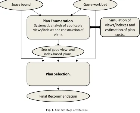
As shown in Figure 1, our architecture has two stages: (1) A search for sets of competitive plans for the input queries (“plan enumeration”), and (2) Selection of one efficient plan for each input query (“plan selection”). The first stage begins with a query workload and, optionally, a space bound. It produces a set of plans and corresponding views so that there is at least one plan for each query. The output of stage one, along with the original query workload and space bound, becomes the input to stage two. (The space bound is optional as input to stage one because different bounds can be introduced in stage two.)
All problem-specific details are encapsulated in stage one of our architecture. For example, we can restrict the nature of the queries allowed, the types of views, the operators, etc. The only output from stage one is a set ofIDsof plans and of the views used in the plans. In fact, nothing about the details of the plans or views needs to be conveyed to stage two other than (a) the set of plans for each query; (b) the set of IDs of views required by each plan; (c) the cost of each plan; (d) the space required by each view; and (e) the space bound. Stage two is then free to solve a generalized knapsack problem: find the lowest-cost plan for each query such that the total space used by the required views is no greater than the given bound. An ILP formulation of this problem is given in [17]. While a large variety of exact algorithms and heuristics can be employed in stage two (see [17] for one approach), the last 10-15 years have seen the emergence of sophisticated commercial solvers directed at general problems in mathematical programming, such as integer programming, quadratic program-ming, and constraint programming. These include Ilog CPLEX [10], COIN-OR [32], and SAS/OR [33]. Their superiority over problem-specific heuristics and algorithms has been demonstrated in various domains, including design automation [34]. Furthermore, these solvers are enhanced regularly with significant improvements that directly impact their use in application areas where they may not have been competitive a few years ago.4
Another major advantage of the general-purpose solvers is their ability to incorporate new constraints and problem-specific heuristics at runtime via callbacks. The solver can be configured so that, at any point during the search, the current state can be used to decide whether to (a) add a constraint, (b) invoke a heuristic, or (c) to bias the search in a particular direction.
Our work strives to exploit the performance of CPLEX and other ILP solvers by transforming ADP instances into ILP instances. The biggest challenge is that, for a given query workload, the number of potential views, indexes, and (by extension) plans grows exponentially or worse in the number of queries. This combinatorial
4 Our collective experience bears this out. The [34] paper, based on CPLEX 7.5, reports instances where an approach that
Plan Enumeration.
Systematic analysis of applicable
views/indexes and construction of
plans.
Plan Selection.
Query workload
Space bound
Final Recommendation
Simulation of
views/indexes and
estimation of plan
costs.
Sets of good view‐ and
index‐based plans.
explosion plagues all heuristics and algorithms for view (or index) selection, either directly, or in most cases indirectly (for example, when a heuristic is only able to explore a small portion of the solution space).
Our architecture demonstrates that (a) the difficulties can be isolated (in stage one) and, for special cases of practical interest, overcome; and (b) even large instances of the ILP formulation in stage two can be solved efficiently.
Given the fact that the input to stage two abstracts the details of the original ADP instance and reduces the problem to an ILP model, the following propositions hold with respect to any exact stage-two AlgorithmA.
Their correctness derives directly from the design of our architecture.
Proposition 1. If the set of plansP has a subset P" such that P" includes at least one optimal plan for each
query and the views and indexes required byP"satisfy the space limitB, then any solution produced by Algorithm
A using the subsetP" will be optimal with respect to the original query workload and B.
Proposition 2. If the set of plans P has a subset P" such that the total cost of plans in P" is within relative
error"of the optimum cost for the original query workload and the views and indexes required byP" satisfy the
space limitB, then any solution produced by AlgorithmA will be within relative error" of optimal with respect
to the original query workload and space B.
In other words, the quality of the output of stage one directly determines the quality of the solution produced by our architecture.
Most of the remainder of the paper is devoted to implementations of stage one of our architecture for variants of the CQAC problem (Section 4), and to experiments confirming the competitiveness of our approach (Sec-tion 5). Finally (Sec(Sec-tion 6), we discuss extensions of the CQAC problem that can be handled by straightforward generalizations of our algorithms of Section 4.
4
Efficient Evaluation Plans for CQAC Queries
We present two variations of a specific algorithm implementing stage one of our architecture of Section 3. The algorithm is applicable to conjunctive queries with arithmetic comparisons (CQAC queries) in the problem input, and considers views and rewritings in the language of CQACs. One variation that we propose is an optimal algorithm in the sense of Proposition 1. The other generates fewer plans, trading optimality for efficiency. As our experiments in Section 5 show, the solution quality of the second approach is still quite good, optimal or almost so for small instances, superior to those of [3] for larger ones (for which the optimum is not known). Please see Section 6 for a discussion of more general classes of problem inputs that are covered by generalizations of these algorithms.
The remainder of this section proceeds as follows. In Section 4.1 we illustrate the main idea via an algorithm that finds an optimal plan for a single CQAC query. This algorithm, while of no interest in this context to our architecture, introduces the framework for our proposed stage-one algorithms for multiple input queries. In Section 4.2 we deal with the complications arising with multiple queries, and show that our algorithms still maintain optimality. At the end of Section 4.2 we present twopruning rules that significantly reduce the overall number of plans under consideration. One of these maintains optimality in the sense of Proposition 1, the other drastically reduces the number of plans at the expense of the optimality guarantee, but still yields high-quality solutions, see Section 5.
4.1 Finding Efficient Plans for a Single CQAC Query
The standard System-R-style optimizer [35] uses dynamic programming(DP)to find best plans for all subqueries of a given query, in order of increasing sizes. For each subquery, it creates new plans that join plans for the component subqueries. After that, it chooses and saves the cheapest plan for each “interesting order” of tuples. We adapt this algorithm to ADR, with two important modifications:
1. In addition to the plans created by joins of subplans, we consider one more plan: a simulated covering view — a view that matches the subquery exactly (if not already in the database). This allows us to consider plans with a variety of combinations of simulated views.
2. We keep allrelevant5 plans for each subquery. This is important for feasibility: The views required by the plan for each of the subqueries may satisfy the space bound, but the total space bound of those views when the plans are joined may fail to do so.
5 Even when optimal plans are sought, it is not necessary to keep all plans. The number of plans can be pruned
We introduce our approach by way of Algorithm SingleQueryPlanGen in Figure 2. The algorithm (as
well as the algorithm of Section 4.2) finds allbushy plans of a query, thus ensuring optimality. Most modern optimizers limit themselves to the smaller (incomplete) search space of linear plans. We could do the same and obtain much more efficient algorithms.
Algorithm 1:SingleQueryPlanGen
Input: database statistics (see Section 2), CQAC queryQ, space boundB
Output: a set of all plans forQthat require at mostB additional space foreach subquery qof Qin the order of increasing length do
1
foreach split of qinto two smaller subqueriesq1 andq2do
2
foreach pair of plansp1 andp2 ofq1 andq2 do
3
if total space required by simulated views ofp1 andp2 is at mostB then
4
create planpby joiningp1 andp2;
5
savepinto the set of plans forq;
6
if the size of the answer toq is at mostBthen
7
simulate viewvq with the answer toq; 8
create planpbased onvq; 9
save planpinto the set of plans forq;
10
PrunePlans(q);
11
returnset of plans forQ 12
Fig. 2.Constructing (possibly view-based) evaluation plans for a single CQAC query.
In the algorithm above, each subquery is represented with a node that contains a list of plans. The nodes are organized into theDP lattice, with single-table subqueries at the bottom, followed by the subqueries based on two tables, etc., and with a single node corresponding to the whole query at the top.
The algorithm investigates the nodes of the lattice in the bottom-top manner and builds the plans using two technics: (1) joining of plans for smaller subqueries (lines 2-6); (2) creating plans that use only one view containing the answer to the subquery (lines 7-10).
We assume that the operations in lines 4-6 can be executed in constant time. Suppose, subquery q1 has length k1 and q2 has length k2. Then, in the worst case, in the for-loop in line 3, we consider joins of 2k1−1 plans forq1 with 2k2−1plans forq2, for a total of 2k−2 joins, wherek=k1+k2 is the length ofq. The for-loop in line 2 considers k−1 splits of subquery qof length kin two smaller subqueries. Thus, the total number of
join-based plans that we build for a subquery of sizek is (k−1)2k−2. After that, in lines 7-10, we create one more plan that is based on a view corresponding to the answer to subquery q. We assume that creating such
plan takes approximately the same amount of time as creating a join based plan. Note that we keep only 2k−1 plans for q, because some of the plans correspond to the same rewriting, and we keep only the best plan for
each rewriting.
Thus, the overall complexity of the algorithm is proportionate to
n %
k=1
(n−k+ 1)((k−1)2k−2+ 1)∼O(n32n),
wherenis the number of tables in the query.
Observe that for a given subquery, the total number of possible plans may be exponential in the number of tables, attributes, and so on. Thus, considering all of them may become prohibitive even for small-size queries. One of the contributions of this work is a set of pruning rules that allow us to avoid considering large parts of the space of the (possibly view-based) plans for the input queries.
Definition 2. Let p1 andp2 be two plans for the same subquery. Ifp1 andp2 return the same tuples in exactly the same order, such that cost(p2)≤cost(p1) and weight(p2)≤weight(p1)each hold, with at least one strict inequality, then planp2 dominates plan p1.
Procedure PrunePlansin Algorithm 2 removes planpfrom the list of plans for a subquery wheneverpis
dominated by another planp".
Example 2 illustrates the work of AlgorithmSingleQueryPlanGen.
Example 2. Consider the query
SELECTA.a, B.c
FROM A, B, C
WHERE
A.b=B.bAND
B.c=C.cAND
C.d≤100
from Example 1 and suppose the database is populated as in Figure 3.
A a b 1 2 2 4 3 4 3 5 4 6
B b c 2 2 2 5 3 4 4 5 4 3
C c d 2 50 3 100 4 150 5 200
Fig. 3.Sample database.
AlgorithmSingleQueryOpt starts by creating plans for the subqueriesA, B, andC based on sequential
scans of the corresponding tables: call thesepA,pB, andpC, respectively. A second alternative forCis to create
a view for C(c, d)d ≤100: call this planpC,2. The plan pC requires no additional space and has cost 4 while
pC,2requires space 2 and has cost 2.
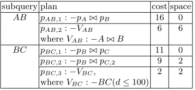
Figure 4 shows the plans for subqueries of length 2. In each case, the first is derived by joining scans of two base tables and the last from a view created specifically for the subquery. In the case of BC, the middle
alternative arises because there was a second plan for subquery C(d ≤100). Because of the pruning rule the
planpBC,2 is eliminated: it is more expensive thanpBC,3 and uses the same amount of space.
subquery plan cost space
AB pAB,1:−pA!" pB 16 0
pAB,2:−VAB 6 6
whereVAB:−A !" B
BC pBC,1:−pB!" pC 11 0
pBC,2:−pB!" pC,2 9 2
pBC,3:−VBC, 2 2
whereVBC:−BC(d≤100)
Fig. 4.Plans for the 2 subqueries of length 2.
plan id plan cost space
1 pA!" pBC,1 19 0
2 pA!" pBC,3 10 2
3 pAB,1!" pC 23 0
4 pAB,1!" pC,2 21 2
5 pAB,2!" pC 13 6
6 pAB,2!" pC,2 11 8
7 VAC(a, c) 3 3
whereVAC(a, c) :−A(a, b)B(b, c)C(c, d)d≤100
Fig. 5.All available plans for queryQwith unrestricted amount of the available disk space.
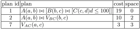
plan id plan cost space
1 A(a, b)!"[B(b, c)!"[C(c, d)d≤100]] 19 0
2 A(a, b)!" VBC(b, c) 10 2
7 VAC(a, c) 3 3
Fig. 6.Ranking of view-based plans for queryQ.
Theorem 1. Algorithm SingleQueryPlanGen returns all view-based plans that do not violate the input
space bound and are not dominated by other plans.
We prove, by induction on the length of the (sub)query q, that the list of plans forqin Algorithm Single-QueryOptincludes all plans that are within the space bound and are not dominated. This is clearly true for
queries on the original base tables.
Letpbe a plan for (sub)queryqand supposepobeys the space bound and is not dominated. Ifpis simply
the view representing q, then the algorithm adds it to the list in lines 8-10. Otherwisep is p1 #$ p2 possibly followed by some selections, wherep1 and p2 are plans for smaller subqueriesq1 and q2, respectively. Sincep satisfies the space bound, so dop1andp2. And neitherp1norp2is dominated. If, for instance,p1was dominated byp"
1, then planp"1#$ p2 would dominatep, contradicting the fact thatpis not dominated.
By induction we know thatpi is on the list forqi fori= 1,2 andpis considered in the loop in line 3 of the
algorithm.
!
4.2 Finding Efficient Plans for Multiple CQAC Queries
In this subsection we discuss how to adjust the algorithm of Section 4.1 to work for multiple CQAC queries. Our proposed algorithm is applicable tochained queries.
Definition 3. A set of queriesQis a set of chained queries, if there exists a sequence of base tablesL(possibly,
with several occurrences of the same tables), such that, for each query q of Q, its set of tables matches with a
subsequence ofL, and the joins in q occur only between neighboring tables inL.
We refer toLas theglobal chain. In this work, we do not address the question of constructingL. We assume
that the global chain can be easily deduced from the database schema. Note that the queries in the TPC-H benchmark [36] are chained queries on a chain of length 9, with possibly some additional queries that turn the chain into a cycle or follow a single branch away from the chain. The case of the branch can be incorporated into our approach (see Section 6), while the cycle is currently under investigation.
A naive approach to processing problem inputs with multiple chained queries would be to find plans for each input query separately using the algorithm of Section 4.1. This approach has several obvious problems:
1. One problem is with efficiency, especially when queries have common parts, as in this case we may end up doing some of the work repeatedly.
2. If we consider queries in isolation, we can miss some structures that are suboptimal for single queries, but are beneficial for groups of queries. For instance, if one query has an arithmetic comparison(AC)0≤B≤3,
whereB is an attribute name, and another has 1≤B≤4, then materializing a view with AC “0≤B≤4”
3. Finally, the pruning rule for the single-query algorithm might remove plans that are needed for an optimal solution. Example 3 describes such a situation.
Example 3. Consider two queriesQ1:-ABCandQ2:-BCD. We omit attributes, because they are not relevant here.
Suppose, in the node corresponding to subgoalsABC, we have two plansp1:-V1#$Candp2:-A#$V2, whereV1:-AB
andV2:-BC; and in nodeBCDwe have p3:-V2#$Dandp4:-B#$V3, whereV3:-CD. Let
cost(p1)< cost(p2)
cost(p4)< cost(p3). and
weight(V1)< weight(V2)
weight(V3)< weight(V2).
Following the single-query pruning rule, we would eliminate bothp2 andp3, because they are less efficient than
p1 andp4, respectively. If we consider the combination of plans (p2, p3) versus plans (p1, p4), then (p1, p4) has lower cost, but the relative weights of the plan pairs are unknown:
cost(p1) +cost(p4)< cost(p2) +cost(p3)
weight(V1) +weight(V3) ? weight(V2)
Ifweight(V1) +weight(V3)> weight(V2), then the combination (p2, p3) becomes a viable option. Thus, the single-query pruning rule is not valid for multiple queries.
In what follows we discuss the basic framework of a multi-query algorithm and two pruning rules for it, one that guarantees the presence of an optimal solution for each query, the other trading off optimality for efficiency. Chained Queries without ACs.For chained queries without arithmetic comparisons (ACs), our algorithm uses the same DP structure as the single-query case, with one important difference: some subchains of the combined chain are not subqueries of any query and do not require plans to be created for them.
Consider an illustration. Suppose we have two queries Q1 : −ABCD and Q2 : −CDE. (This format of defining the queries enumerates just the predicate names of all the relational subgoals of the queries.) Then the combined chain isABCDE. SubchainBCDE is not a part of either query, nor is ABCDE – we do not need
plans for either of them. The DP lattice for the case of multiple queries resembles a collection of mountain peaks as illustrated in Figure 7, which shows the lattice for three queries on a combined chain of length 8. In this diagram, circles represent subchains for which we need to construct plans. Examples of subchains for which we do not need to construct plans areD46, D25,andD36. (NotationDij, with i < j, refers to a chain of subgoals
i, i+ 1, . . . , j−1, j.)
Our pruning rule for the case of a single query may not be correct for the case of multiple queries. Suppose that in the multi-query case, we prunep1because its cost is higher than that ofp2, andp1uses at least as much space asp2. In the multi-query situation, if we replace all occurrences ofp1 withp2 then the overall cost of the solution will decrease but the total size of views used by the plan may actually increase, as the views used by
p1might be useful for evaluating other queries. Thus, removal ofp1 might actually eliminate feasible plans that take advantage of the space savings when views are used by plans for more than one query.
To avoid this problem, we propose the following definitions.
Definition 4. For a given set of queries Q, we say that a view v is exclusive if it can be used by exactly one
query inQ.
Definition 5. The exclusive weightof plan p,ew(p), is the total size of the exclusive views ofp.
Definition 6. Let p1 andp2 be two plans for the same subquery. Ifp1 andp2 return the same tuples in exactly the same order, such that cost(p2) ≤ cost(p1) and weight(p2) ≤ ew(p1) each hold, with at least one strict inequality, then planp2 globally dominatesplan p1.
In our algorithm MultiQueryPlanGen(Algorithm 2), procedurePrunePlans removes from the list of
plans for a subquery all plans psuch that pis globally dominated by another plan p" for the same subquery.
D1
D2
D3
D4
D6
D7
D8
D12
D67
D13
D45
D34
D23
D58
D68
D57
D35
D24
D14
D5
D78
D56
Q
1Q
2Q
3Fig. 7.Example of DP lattice for multiple chained queries. (Dij, withi < j, denotes a chain of subgoalsi, i+1, . . . , j−1, j.)
weight — sum of sizes of all used views — of each plan. Then we can executePrunePlanseither by comparing
each pair of plans or, more efficiently, by first sorting the plans by cost or by maintaining a search tree. Adding arithmetic comparisons. We now discuss what happens when we allow selection conditions in the WHERE clause of the input queries. For ease of exposition, we assume that all the selection conditions are range (i.e., inequality) arithmetic comparisons (ACs), although, as we explain later, most of the techniques that we discuss here apply to other types of selection conditions.
In presence of ACs, our algorithm needs several adjustments. First, each node of the lattice implied by our algorithm SingleQueryPlanGen (Algorithm 1) corresponds to a subset of tables (relational subgoals of a
query) and contains plans for the subqueries based on these tables. But when the problem input has multiple queries with different selection conditions, two plans built on the same set of tables might differ with respect to their selection conditions and not be usable for the same set of queries. As a result, the same node might contain plans for different subqueries. Therefore, for each plan, we need to keep a list of queries that can use this plan.
Second, we must take care of so-calledmerged views – views that are usable by more than one query. If we have two queries that use the same subset of tables but different sets of ACs, then it may benefit both to create a merged view whose set of ACs is the disjunction (i.e., OR) of the ACs of the queries.
It is easy to see that for the case where three queries overlap on the same set of subgoals, we may need to create one merged view for each pair of the queries, and one merged view for all three queries. Although in theory this means that the number of merged views that we need to create is exponential in the number of queries, in practice this number is much lower. Examples that follow illustrate that the actual number of merged views may not be that large in practice.
Suppose we haven >2 queries that overlap on the same larger chain (set of tables). Suppose queryQ1has ACs on attributes B1 and B2, queryQ2 has ACs onB2 andB3, etc. We can assume that the attributes that do not have ACs on them have ACs that match their whole domains. Then, when we merge views for Qi and Qj, such that |i−j| >1, for any attribute ak, the disjunction of constraints from Qi and Qj is a constraint
that covers the whole domain ofak, which means there is no AC onak. The same is true for any subset of the
queries containing more than two queries. Therefore, in this case, we have onlyn−1 possible merged views. For another possible scenario, suppose that one query has AC (B >100) on attributeB, and another query
has AC (B <200). In this case, the merged view for these two queries will have attributeB unbounded.
Our approach to generating efficient query plans for the CQAC version of problem ADR is encoded in algorithmMultiQueryPlanGen(Fig. 8). The algorithm uses two auxiliary structures:plans(q) is the list of
Algorithm 2:MultiQueryPlanGen
Input: database statistics (see Section 2), set of CQAC queriesQthat together form chainH, space boundB
Output: a set of plans for each query inQ, containing optimal solution to ADR foreach sub-chainq ofH in the order of increasing length do
1
foreach splitq into two smaller sub-chainsq1 andq2 do
2
foreach pair of plansp1∈plans(q1) andp2∈plans(q2)do
3
if queries(p1)∩queries(p2)%=∅AND total weight ofp1 andp2 is at mostB then
4
create planpby joiningp1 andp2;
5
queries(p) =queries(p1)∩queries(p2);
6
savepintoplans(q);
7
letQ! be the set of queries for whichqis the subset of tables;
8
foreachk⊆Q! do
9
simulate viewvwhich is the result of the join of tables inqwith the disjunction of the sets of constraints
10
of queries inkapplied to it; if the size ofvis at mostB then
11
create planpbased onv;
12
initialize queries(p) with indexes of queries ink;
13
save planpintoplans(q);
14
PrunePlans(q);
15
returnset of plans for each query in Q 16
Fig. 8.Constructing (view-based) evaluation plans for multiple CQAC queries.
Ifm queries overlap on a subchain of lengthn, the total number of view-based rewritings for this subchain
is proportional to O(2nm). The intuition behind this is the same as for the single-query case, but this time,
for a common for m queries subchain, in the worst case, we can create 2m different views. Thus, the overall
complexity of Algorithm 8 isO(n32nm).
Theorem 2. Algorithm MultiQueryPlanGen returns a set of view-based plans P such that there exists S⊆P whereS is an optimal set of plans.
Using the same technique as in the proof (by induction) of Theorem 1, we can prove that without function
PrunePlans the algorithm constructs all possible plans that use exclusive or merged views. The only thing
that remains to be proved is that our pruning function retains an optimal solution.
Suppose an optimal solutionSis not among the plans returned by AlgorithmMultiQueryOpt. This means
there exists planpfor queryq, wherepis in some optimal solution and not in the output of the algorithm. The
absence ofpmeans that, for some subplanpsofp, there is another subplanp"
sthat globally dominatesps. Note
that, by the definition of global domination, we can replace ps byp"
s inpwithout increase in the cost ofp. At
the same time, when we replace ps byp"
s, we reduce the total weight of the solution by at least the exclusive
weight of ps and increase it by at most the total weight of p"s. Thus, by the definition the global domination,
the total weight of the solution does not increase. Therefore, replacingpsbyp"sinp, we obtain a solution which
is at least as good asS; and, if we find in solutionS all such dominated subplans and replace them with their
dominating alternatives, we get a solution which is at least as good as S and is among the plans return by
AlgorithmMultiQueryOpt.
! Theorem 2 is a very important result. It means that AlgorithmMultiQueryPlanGenperforms a
system-atic investigation of the search space of view-based plans and returns a (reduced-size) list of plans that contains an optimal solution. Thus, the solution quality of the two-stage architecture that we presented in Section 3 depends only on the quality guarantees of the algorithm used in stage two of the architecture. Combined with Propositions 1 and 2, this result provides strong optimality guarantees for our overall architecture when applied to the CQAC class of problem inputs considered in this section.
More aggressive pruning. The strong point of Algorithm MultiQueryPlanGenis that it preserves
In Example 3, we demonstrate that the pruning rule that we used in our single-query algorithm (see Sec-tion 4.1) does not guarantee optimality if used for the multiple-query case, as it does not account for the views that are shared by multiple queries. At the same time, our experiments (Section 5) suggest that the single-query rule, even if applied to the case ofmultiple queries,does not significantly reduce the quality of the solution.
Although the “single-query” aggressive rule of the previous paragraph prunes many more plans than the conservative one, it is still instance dependent and does not guarantee convergence within the allocated time. In other words, we do not know a-priori how many plans the aggressive rule will prune for a given instance, and thus how fast the algorithm will find a solution. We might get really unlucky, in that the aggressive pruning might not prune any plans at all. In the worst case, we can still get exponential runtime complexity in the number of queries, tables, selection conditions, and attributes for each subproblem. To counter this problem, the idea of our second aggressive pruning rule is to limit the number of plans we keep for each subproblem: we keep onlykplans with the largestprof it∗queries/size, whereprof itis the decrease in cost offered by the plan
(over use of base tables),queries is the number of queries that can use the plan, andsize is the total size of
the views used by the plan.
5
Experimental Results
The experiments reported in this section address two questions: (a) How does our two-stage approach compete with a relaxation-based approach (RBA), such as that of [3]? (b) Can we safely assume that stage two is not the bottleneck when using CPLEX [10]? Our extensive and thorough investigation gives a positive response to each question.
We begin in Section 5.1 with a discussion of how we generate random problem instances with characteristics typical of those arising in practice. In Section 5.2 comparisons with the RBA are reported for a large number of instances. Scalability of the stage two computation using CPLEX is demonstrated in Section 5.3.
All of our experiments were done on an AMD Athlon(tm) 64 X2 Dual Core Processor 5200+, with 2 MB of L2 cache, and 4 GB memory, running Red Hat Enterprise Linux 5. The programs were implemented in C++ and compiled using gcc version 4.1.2. We called CPLEX version 11.0 directly from our software.
5.1 Instance Generation
Query instances derived from benchmarks such as TPC-H [36] tend to be small, making it difficult to test scalability, and that algorithms that work well for them may not perform as well in general. Random instances, on the other hand, have to be generated carefully to reflect what occurs in practice. We now give a detailed description of how the problem instances for stage one were generated. We do experiments on both types of instances. This section discusses the details of random instance generation.
Relationships among queries were determined by three structural parameters: M = the length (number of
tables) of the global chain, N = the number of queries, andL= the maximum length of the subchain for any
query. The choice of the values of the parameters has an impact on the degree to which queries overlap: if L
and/orN is large w.r.t.M, there is likely to be much overlap.
For each of theN queries we generate a random integerrin [1, L]; thisris the length of the subchain for that
query. The position of the query in the global chain is determined by choosing a random integersin [1, M−r]
to be the first table of the query. We used fixed values of M and L for increasing the number of queries. For N = 22, the choiceL= 8 reflects the nature of the TPC-H workload. Our choice ofM = 20 is somewhat larger
than the longest global chain in TPC-H, but is typical of databases with a large number of attributes.
We also used a collection ofnumerical parameters to determine the sizes of base tables and related quantities that affect cost and space usage.
– Wmin and Wmax are the minimum and maximum number of tuples, respectively, in a base table; we call
the number of tuples the size from here on6; these directly affect both space of a view and cost of a plan;
Wmax is also the upper limit on the number of values an attribute can take, its value counter (v.c.); We
used Wmin= 5,Wmax= 100 to avoid arithmetic overflows when computing sizes/costs with longer chains.
– B is the space bound – limit on the amount of available disk space in addition to that used by the base
tables; our experimental results depend on the choice of B: a problem instance is trivial if B is the total
size of all query results (just create a view for each query) and becomes harder asB decreases.
6 Size usually means number of bytes, but, in order to avoid introducing another variable to the instance generation,
The global chain ofM tables, numbered 1 toM, containsM + 1 attributes, numbered 0 toM. Attributes
1 toM −1 are join attributes; a join involving tablesi and i+ 1 uses join attribute i. First the v.c. of each
attribute and the size of each table is chosen to be a random integer in [Wmin, Wmax].
Further, for each table, with probability P = 0.8 we decide whether one of its two attributes is a key
attribute, and, if so, pick one. In practice joins are frequently done on key attributes – the value chosen here is based on the TPC-H workload. A potential conflict between table size and key attribute v.c. may arise at this point. When this is the case the table size is set to be the v.c. of the key attribute rather than the previous randomly chosen value.
Since the set of values taken on by an attribute, itsglobal domain, is independent of that taken on by other attributes, we can safely assume that all global domains are integer intervals [0, w], wherew is the v.c. of the
attribute.
When an attribute is not a key attribute, a table does not necessarily contain all of its values. For a given tablei and join attributej=i−1 ori, the local domain i, jis the set of values in tablei for attributej. The
v.c. of each local domain i, j is chosen to be a random integer that is no larger than either the size of table i
or the v.c. of attributej. Each local domain is a sub-interval of the corresponding global domain, also chosen
randomly depending on the v.c.
The last set of random choices is that ofconstraints on the attributes. In practice, some attributes, such as invoice date, are more likely to be subject to constraints, i.e., are more important than others, such as customer id. Hence we choose animportance for each attribute, a random real numberI from [0,1].
A queryqon tablesitojinvolves attributesi−1 toj. For each of these attributes we must decide whether
the attribute has a constraintfor that query; this is true with probabilityI, the importance of the attribute. If
there is a constraint, it is chosen to be a random sub-interval of the attribute’s global domain. Note that both the decision about whether to include a constraint and the actual interval are independent for each query.
5.2 Comparisons with RBA
The RBA algorithm we use for comparison purposes is the one described in [3]. It consists of two main stages: (a) choose a set of physical structures (i.e., views or indexes) that is guaranteed to result in an optimal con-figuration, but may take too much space; and (b) “shrink” it using transformations, such as view and index merging, index prefixing, etc., that reduce the total required space.
In the experiments comparing our two-stage approach with the RBA of [3] we examined the quality achieved by each approach within a specified time period. Our own implementation of [3] was used since we did not have access to the code for it.7 Any comparison using time as a measure may therefore not be representative of the actual relative performance of the two approaches. Thus we use a combinatorial measure, as follows.
In the physical database design literature it is a common practice to use the total number of query-optimization calls as a measure of time spent on query-optimization. We use a more fine-grained unit of time — size estimation. For each operator in a plan tree, the optimizer estimates the size of the results, the execution cost, and the order of tuples of the result. Thus, any query-optimization call consists of a series of size and statis-tics approximation calls. Although size estimations are not the only operations performed by the optimizer, they tend to dominate the runtime of query optimization.
We ran the RBA algorithm on each instance until it had done as many size estimations as our Multi-QueryPlanGen(Section 4) using the single-query pruning rule; we refer to this algorithm asAR,aggressive
(pruning) rule. We then compared the solution quality of the two algorithms.8 Fig. 9(a) shows that in almost all cases our algorithm achieves higher quality solutions.
In a few cases RBA failed to find a feasible solution at all. To make sure that the cutoff did not preclude solutions that were almost encountered by RBA, we also compared the performance with RBA allowed four times as many size estimations as our algorithm, see Fig. 9(b). Note that the RBA’s performance did not improve much vs. AR even when allowed four times as many size estimations. In fact in only three (out of 250) cases, RBA was able to improve its solution in comparison to AR.
In both experiments the results differ depending on the relationship between the space bound and the total size of the query results. What both parts of the figure show is that our approach gets better relative to RBA as
7 Microsoft Research is currently unable to distribute the research prototype externally due to IP considerations. 8 Stage two using CPLEX is also executed following our MultiQueryPlanGenof Section 4. This part took only a
AR is better than RBA
AR is the same as RBA
AR is worse than RBA
50
AR!is!better!than!RBA
AR!is!the!same!as!RBA
AR!is!worse!than!RBA
40
45
s.
35
40
a
n
ce
s
25
30
in
st
a
20
25
er
!
o
f
!
10
15
u
m
b
e
5
10
N
u
0
0.1
0.3
0.5
0.7
0.9
Space bound as fraction of total size of query answers
Space
!
bound
!
as
!
fraction
!
of
!
total
!
size
!
of
!
query
!
answers.
(a) RBA is allowed the same number of size estimations.
AR is better than RBA
AR is the same as RBA
AR is worse than RBA
45
50
AR
!
is
!
better
!
than
!
RBA
AR
!
is
!
the
!
same
!
as
!
RBA
AR
!
is
!
worse
!
than
!
RBA
40
45
35
40
ce
s.
25
30
n
st
a
n
c
20
25
o
f
!
in
10
15
m
b
er
!
5
10
N
u
m
0
0.1
0.3
0.5
0.7
0.9
Space bound as fraction of total size of query answers
Space
!
bound
!
as
!
fraction
!
of
!
total
!
size
!
of
!
query
!
answers.
(b) RBA is allowed four times as many size estimations.
Aggressive!pruning!rule!with!max.!number!of!plans!10
Aggressive!pruning!rule!with!max.!number!of!plans!20
A
i
i
l
i h
li i d
b
f l
160
Aggressive!pruning!rule!with!unlimited!number!of!plans
140
.
100
120
!
sec
.
80
100
im
e,
60
R
u
n
ti
40
R
0
20
0
50
55
60
65
70
75
80
Number!of!queries
Fig. 10.Scalability of aggressive pruning rules.
the problem gets harder, i.e., less space is available. In fact the difference becomes dramatic with only a slight increase in difficulty.
Recall that the runtime of AR is exponential in the worst case. Even in practice its runtime increases dramatically with increasing query length. To mitigate this, we experimented with a version of AR that sets a limit on the maximum number of plans kept for each subquery. The choice of plans is made heuristically using thek plans with largestprofit∗queries/size, whereprofit is the decrease in cost offered by the plan (over use
of base tables),queries is the number of queries that can use the plan, andsizeis the total size of the views in the plan.
Fig. 10 shows how the runtime increases with query workload for k = 10 and 20, i.e., AR10 and AR20,
versus the original AR. Here, the actual runtime can be used, because we compare three variations of the same algorithm. The much slower growth for AR10 and AR20 is evident. We still need to demonstrate that these algorithms are competitive when it comes to solution quality.
Fig. 11 shows the performance of AR20 vs. RBA using the same setting as that of Fig. 9. The superiority of AR20 w.r.t. solution quality is not as dramatic as with AR, but still clear. Whereas AR wins practically all the time with the space bound less than 100% of the total size of query answers, AR20 catches up gradually and attains superiority at 50%. After that, the relative results do not change significantly.
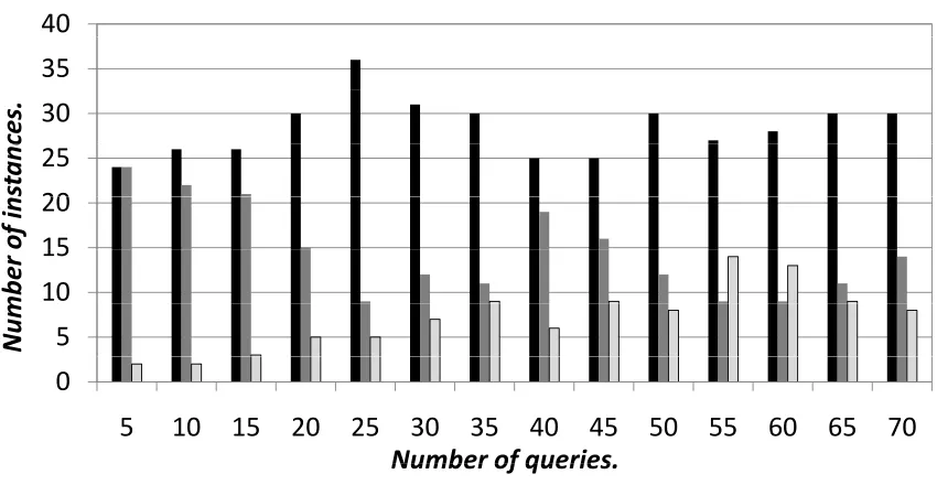
Another way to evaluate AR20 is how its performance vis a vis RBA scales with the number of queries. Since AR20 makes significantly fewer size-estimate calls than AR, we end up allowing fewer size estimates for RBA. When the space bound is 50% of the total size of query answers – Fig. 12 – the results are mixed; AR20’s advantage in “speed” is offset by poorer relative solution quality. However, when the space bound is 10% of the total size of query answers, the instances are much harder for RBA, while AR20 is still able to come up with significantly better solutions.
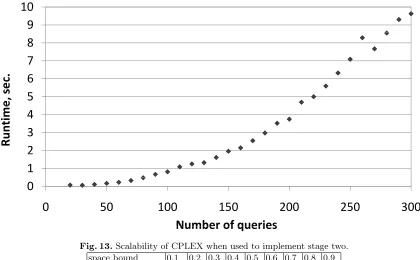
5.3 Scalability Results
One concern with our two-stage architecture is that the second stage, which solves a generic integer programming problem instead of using problem-specific techniques, might incur prohibitive runtime. Our experiments suggest otherwise.
AR20 is better than RBA
AR20 is the same as RBA
AR20 is worse than RBA
40
AR20
!
is
!
better
!
than
!
RBA
AR20
!
is
!
the
!
same
!
as
!
RBA
AR20
!
is
!
worse
!
than
!
RBA
35
25 30
ce
s.
20 25
n
st
a
n
c
15 20
o
f
!
in
10
m
b
er
!
5
N
u
m
0
0.1
0.3
0.5
0.7
0.9
Space bound as fraction of total size of query answers
Space
!
bound
!
as
!
fraction
!
of
!
total
!
size
!
of
!
query
!
answers.
Fig. 11.AR20 versus RBA for different space bounds.
queries can be solved in a few seconds.9The largest instance that we were able to solve within 10 minutes using CPLEX had 800 queries, 1074 plans per query, and 6886 views.
5.4 Comparison on TPC-H workload
In this section we present results of the comparison of AR and RBA on TPC-H-shaped instances. As we said earlier, our experimental framework can deal only with singe-block chain queries with range constraints. Thus, we preprocessed all queries of the TPC-H workload to match them with our template. One interesting fact is that almost all queries of TPC-H are chain queries, and they can be combined into a global chain consisting of 9 table:
region−nation−supplier−partsupp−lineitem−orders−customer−nation−region
Note that this chain has two occurrences of tables regionand nation. For our model, it is not important,
because we treat them as different tables.
The TPC-H specification gives guidelines for creating queries and allows small variations in the choice of the constraints. Following these instructions, we implemented a query generator with small randomness in the choice of the constraints. Such module can create many similar TPC-H-shaped instances with small variations in constraints.
TPC-H workload consists of 22 queries. As we showed in the sections above, such instances are relatively small for our proposed algorithm. Therefore, we were able to run an experiment on 1000 TPC-H-shaped instances. The average runtime of our algorithm was 3.4 seconds. We allowed RBA to do the same number of size estimations and recorded the solution values returned by the two algorithms. As before, the results differ depending on the relationship between the space bound and the total size of the query results. Figure 14 shows some statistics about the distribution of the relative difference of RBA and AR solution values for various choices of the space bound. Here, we set the space bound as a fraction of the total size of the query answers.
From the results in Figure 14, we can see that the cost of the solution returned by AR is on average 20% to 40% lower than that of RBA. Out of the total of 9000 runs, only in 2 cases RBA returned a better solution than that of AR, and in 25 cases RBA and AR returned the same solution.
9 The jag in the curve appears to be related to the fact that CPLEX 11.0 employs a more aggressive preprocessor when
AR20 is better than RBA
AR20 is the same as RBA
AR20 is worse than RBA
40
AR20
!
is
!
better
!
than
!
RBA
AR20
!
is
!
the
!
same
!
as
!
RBA
AR20
!
is
!
worse
!
than
!
RBA
35
30
ces.
20
25
st
a
n
c
15
20
o
f
!
in
10
15
m
b
er
!
5
N
u
m
0
5
10
15
20
25
30
35
40
45
50
55
60
65
70
Number of queries
Number
!
of
!
queries.
(a) Space bound is 0.5 times total size of query answers.


![Fig. 9. Comparing solution quality of our AR (Section 4) versus the RBA of [3].](https://thumb-us.123doks.com/thumbv2/123dok_us/1743726.1223218/16.612.101.525.127.360/fig-comparing-solution-quality-ar-section-versus-rba.webp)