Statistical Inference for Model Selection.

(1)

ABSTRACT

HU, WENHAO. Statistical Inference for Model Selection. (Under the direction of Eric Laber and Leonard Stefanski.)

Penalized regression methods that perform simultaneous model selection and estimation are

ubiquitous in statistical modeling. The use of such methods is often unavoidable as manual

in-spection of all possible models quickly becomes intractable when there are more than a handful

of predictors. However, such automated methods may fail to incorporate domain-knowledge,

exploratory analyses, or other factors that might guide a more interactive model-building

ap-proach. A hybrid approach is to use penalized regression to identify a set of candidate models

and then to use interactive model-building to examine this candidate set more closely.

In Chapter 1, to identify a set of candidate models, we derive point and interval

estima-tors of the probability that each model along the solution path will minimize a given model

selection criterion, e.g,. AIC, BIC, etc., conditional on the observed solution path. Then models

with a high probability of selection are considered for further examination. Thus, the proposed

methodology attempts to strike a balance between algorithmic modeling approaches that are

computationally efficient but fail to incorporate expert knowledge, and interactive modeling

ap-proaches that are labor intensive but informed by experience, intuition, and domain knowledge.

We envision this approach as being useful in at least two ways: (i) it facilitates interactive,

expert-knowledge driven exploration of high-quality candidate models even when the initial

pool of models is large; and (ii) it provides valid conditional prediction sets for a data-driven

tuning parameter given the observed design matrix and solution path, that is applicable for a

large class of tuning parameter selection methods.

In Chapter 2, we derive an estimator of the false selection rate for each model along the

solution path using a novel variable addition method. The proposed estimator applies to both

(2)

facil-itate interactive model exploration. We characterize the asymptotic behavior of the proposed

estimator in the case of a linear model under a fixed design; however, simulation experiments

show that the proposed estimator provides consistently more accurate estimates of the false

selection rate than competing methods across a wide range of models. With estimated false

selection rates, one may be able to label the solution path with operating characteristics that

are meaningful in a domain context.

In Chapter 3, we describe the developed R package and shiny app. The developed R package

IntVSimplemented the described pseudo-variable methods and built a interactive solution path

using shiny. It allows users interact with solution path of penalized models and observe model

information, e.g., coefficient estimates, false selection rates, AIC and BIC. Besides of the R

package, a shiny website is also built for broader usage. Using the website, users may upload

(3)

(4)

Statistical Inference for Model Selection

by Wenhao Hu

A dissertation submitted to the Graduate Faculty of North Carolina State University

in partial fulfillment of the requirements for the Degree of

Doctor of Philosophy

Statistics

Raleigh, North Carolina

2018

APPROVED BY:

Yichao Wu Arnab Maity

Eric Laber

Co-chair of Advisory Committee

Leonard Stefanski

(5)

DEDICATION

(6)

BIOGRAPHY

The author was born in Yueyang, Hunan, China in September 1991. In 2009, he was admitted

to Sun Yat-sen University (SYSU), where he spent four years on studying Mathematics and

Statistics. In 2010, he met his wife Qian Guan, who was his classmate. After receiving Bachelor’s

degree of Statistics from SYSU in 2013, he attended North Carolina State University for a Ph.D.

in Statistics. Under the direction of Dr. Eric Laber and Dr. Leonard Stefanski, he will complete

(7)

ACKNOWLEDGEMENTS

First of all, I would like to express my deepest gratitude to my advisors Dr. Eric Laber and Dr.

Leonard Stefanski for their continued support and great mentoring. Without their inspiration

and help, this thesis would not be possible. Their passion to research and science set good

examples for me. It is a great experience with them.

I would also like to thanks my committee members Dr. Yichao Wu and Dr. Arnab Maity

for their thoughtful comments. I also thanks Dr. David Skaar for kindly serving as graduate

school representative in my committee.

I would also like to extend my appreciation to all professors in Department of Statistics

at NC State. Dr. Howard Bondell, who was the DGP, served as committee member in my

Oral Preliminary Exam. Dr. Jung-Ying Tzeng, my academic advisor during my first year of

study, provided me valuable guidance. Dr. Wenbin Lu who served as current DGP provide me

tremendous help on graduate studies. I also thank all the great staff in the department.

I would like to thanks all mentors during my internships. At Merck, Dr. Shuyan Wan and

Dr. Frank Liu guided me the research on missing data imputation. At QuantLab, Dr. Areez

Moody taught me how to develop quantitative strategies for trading and understand financial

market. And at SAS, Arin Chaudhuri and Gul Ege provided me suggestions on coding, research

and presentation. Those experiences are invaluable to me.

Thank all my friends and fellow students at NC State and Laber Labs. Thank you!

Last but not least, I could not come this far without the support of my family. My Mom

and Dad are always supportive with their whole hearts. My wife, Qian Guan, have always been

(8)

TABLE OF CONTENTS

LIST OF TABLES . . . vii

LIST OF FIGURES . . . .viii

Chapter 1 Assessing Tuning Parameter Selection Variability in Penalized Re-gression . . . 1

1.1 Introduction . . . 1

1.2 Penalized linear regression . . . 3

1.3 Estimating the conditional distribution of ˆλGIC . . . 4

1.3.1 Conditioning on the solution path . . . 4

1.3.2 Exact distribution of ˆλGIC|(S,b X) . . . 5

1.3.3 Limiting conditional distribution of_bσ2₀ . . . 7

1.3.4 Bootstrap approximation to the distribution of ˆλGIC|(S,b X) . . . 9

1.4 Simulation Studies . . . 9

1.5 Illustrative data examples . . . 13

1.5.1 Pollution and mortality . . . 13

1.5.2 ATV drug resistance . . . 14

1.6 Conclusion . . . 19

1.7 Proof and Technical Details . . . 20

1.7.1 Theoretical results for high dimensions . . . 27

Chapter 2 Variable selection using pseudo-variables . . . 30

2.2 Methods . . . 33

2.2.1 Setup and notation . . . 33

2.2.2 Estimating the false selection rate . . . 34

2.2.3 Computation of pseudo-variables . . . 36

2.3 Simulations . . . 37

2.4 Illustrative examples . . . 39

2.4.1 Prostate cancer data . . . 39

2.4.2 Leukemia cancer gene expression data . . . 42

2.6 Proof and Technical Details . . . 45

2.6.1 Proof of error rate estimation with permutation added . . . 47

Chapter 3 IntVS: An R package for estimating false selection rates in penal-ized regression and interactive variable selection . . . 49

3.2 Methods . . . 50

3.3 The R packageIntVS . . . 51

(9)

3.3.3 Example 3: Estimate False selection rates in SCAD . . . 53

3.4 The shiny website . . . 54

3.4.1 De-biased estimator for Lasso . . . 56

3.4.2 Selective inference . . . 56

BIBLIOGRAPHY . . . 59

Appendices . . . 64

Appendix A Appendix for chapter 1 . . . 65

A.1 Simulation results . . . 65

A.2 Additional results for real-data . . . 67

Appendix B Appendix for chapter 2 . . . 68

B.1 Simulation results forα= 0.1,0.3 . . . 69

B.2 Simulation results without adding permutation . . . 73

B.3 Simulation results for logistic model . . . 75

B.4 Simulation results for Cox model . . . 78

B.5 Pseudo-variables algorithm for screening . . . 81

B.5.1 Theoretical properties . . . 82

(10)

LIST OF TABLES

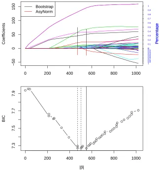
Table 1.1 Discovery rate for p= 20, n= 50 . . . 11

Table 1.2 Discovery rate for p= 100, n= 200 . . . 12

Table 1.3 Coverage Probability. Results are based on 10,000 replicated data sets . . . . 12

Table 1.4 Estimated conditional distribution of the tuning parameter for the mortality rates data. Both the asymptotic normal approximation and the bootstrap had only two support points,{124.21,288.20}. . . 14

Table 1.5 Estimated conditional distribution of the tuning parameter for ATV drug resistance data. . . 17

Table 3.1 Main functions in the R package IntVS . . . 51

Table A.1 Discovery rate for p= 20, n= 50; τ = 0.1 . . . 65

(11)

LIST OF FIGURES

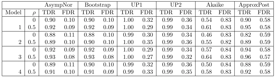
Figure 1.1 The top figure shows LASSO solution path of mortality rates data; The vertical lines above and below x-axis correspond to the distribution estimated by bootstrap and asymptotic normal approximation respectively. The bottom figure shows BIC values for candidate models along solution path. The solid vertical line corresponds to the model with six variables and smallest BIC value. The dashed vertical line corresponds to a model with eight variables. . 15 Figure 1.2 The top figure shows forward stepwise regression solution path of mortality

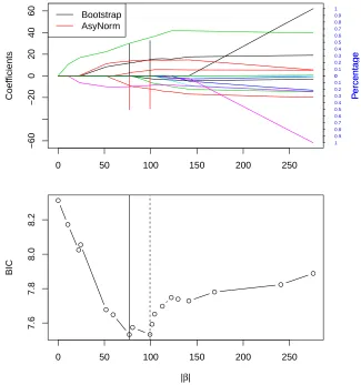
rates data; The vertical line corresponds to the model which minimizes BIC. The bottom figures shows BIC values for candidate models along solution path. The solid vertical line corresponds to the smallest BIC value. . . 16 Figure 1.3 The top figure shows LASSO solution path of ATV drug resistance data;

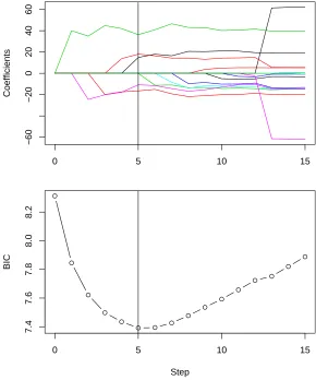
The vertical lines above and below x-axis correspond to the distribution estimated by bootstrap and asymptotic normal approximation respectively. The bottom figure shows BIC values for candidate models along solution path. The solid vertical line corresponds to the model with fifteen variables and smallest BIC value. The dashed vertical lines correspond to model with twelve and ten variables. . . 18

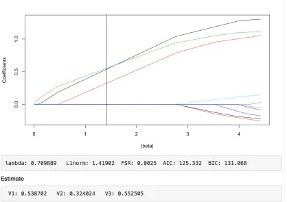
Figure 2.1 Lasso solution path for prostate cancer data. FSR and coefficient estimates are designed to be shown interactively. . . 32 Figure 2.2 Performances under different dimensions at α = 0.2. Left and right figure

shows the average FSR and TSR respectively. The Knockff and Knockoff methods requiren > p and the Wu’s pseudo-variable method requiresn >2p. 40 Figure 2.3 Performances under different correlations at α = 0.2. Left and right figure

shows the average FSR and TSR respectively. . . 40 Figure 2.4 Performances under different coefficient amplitude atα= 0.2. Left and right

figure shows the average FSR and TSR respectively. . . 41 Figure 2.5 Performances under different number of nonzero coefficients at α= 0.2. Left

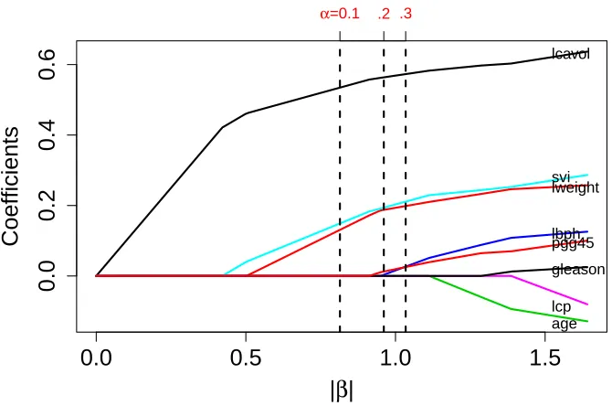
and right figure shows the average FSR and TSR respectively. . . 41 Figure 2.6 Lasso solution path for prostate cancer data. Vertical lines from left to right

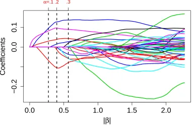
correspond to estimated FSRs ofα= 0.1, α= 0.2, andα= 0.3. . . 42 Figure 2.7 Lasso solution path for leukemia cancer gene expression data. Vertical lines

from left to right correspond to estimated FSRs of α = 0.1, α = 0.2, and α= 0.3. . . 44 Figure 3.1 Interactive plot of solution path; It shows model information including FSR,

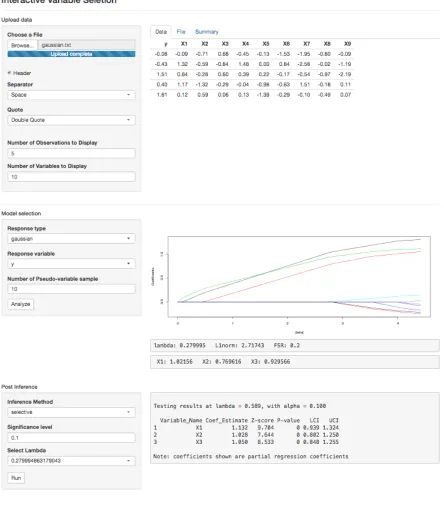
AIC, BIC, and coefficient estimates. . . 55 Figure 3.2 Screen-shot for Shiny Web Application; This application allows users to

up-load dataset, run penalized models, explore solution path interactively and do inference after model selection. . . 58

(12)

Figure B.2 Penalized regression; Performances under different correlations atα= 0.1. . . 69 Figure B.3 Penalized regression; Performances under different coefficient amplitude at

α= 0.1. . . 70 Figure B.4 Penalized regression; Performances under different number of nonzero

coef-ficients atα= 0.1. . . 70 Figure B.5 Penalized regression; Performances under different dimensions at α= 0.3. . . 71 Figure B.6 Penalized regression; Performances under different correlations atα= 0.3. . . 71 Figure B.7 Penalized regression; Performances under different coefficient amplitude at

α= 0.3. . . 72 Figure B.8 Penalized regression; Performances under different number of nonzero

coef-ficients atα= 0.3. . . 72 Figure B.9 Results without permutation added; Performances under different dimensions

atα= 0.2 . . . 73 Figure B.10 Results without permutation added; Performances under different

correla-tions atα= 0.2 . . . 73 Figure B.11 Results without permutation added; Performances under different coefficient

amplitude atα= 0.2 . . . 74 Figure B.12 Results without permutation added; Performances under different number of

nonzero coefficients at α= 0.2 . . . 74 Figure B.13 Logistic model; Performances under different dimensions atα= 0.2. Knockff

and Knockoff+ method only work if n >2p. . . 76 Figure B.14 Logistic model; Performances under different correlations atα= 0.2. . . 76 Figure B.15 Logistic model; Performances under different coefficient amplitude atα= 0.2. 77 Figure B.16 Logistic model; Performances under different number of nonzero coefficients

atα= 0.2. . . 77 Figure B.17 Cox model; Performances under different dimensions atα= 0.2. Knockff and

Knockoff+ method only work if n >2p. . . 79 Figure B.18 Cox model; Performances under different correlations atα = 0.2. . . 79 Figure B.19 Cox model; Performances under different coefficient amplitude at α= 0.2. . . 80 Figure B.20 Cox model; Performances under different number of nonzero coefficients at

(13)

Chapter 1

Assessing Tuning Parameter

Selection Variability in Penalized

Regression

1.1 Introduction

Penalized estimation is a popular means of regression model fitting that is quickly becoming

a standard tool among quantitative researchers working across nearly all areas of science.

Ex-amples include the Lasso (Tibshirani, 1996), SCAD (Fan and Li, 2001), Elastic Net (Zou and

Hastie, 2005), and the adaptive Lasso (Zou, 2006). One appealing feature of these methods

is that they perform simultaneous model selection and estimation, thereby automating

model-building at least partially. This is especially beneficial in settings where the number of predictors

is large, precluding manual inspection of all possible models. However, a consequence is that

the analyst becomes increasingly dependent on an estimation algorithm that has neither the

subject-matter knowledge nor the intuition that might guide a less automated and more

inter-active model-building process (Henderson and Velleman, 1981; Cox, 2001). A hybrid approach

(14)

occurring on a solution path, and then to apply interactive model-building techniques to choose

a model from among these. We develop and advocate such a hybrid approach wherein a set

of candidate models are identified using the solution path, and then models along this path

are prioritized using their conditional probability of selection according to one or more tuning

parameter selection methods. We envision this approach as being useful in at least two ways: (i)

it facilitates interactive, expert-knowledge driven exploration of high-quality candidate models

even when the initial pool of models is large; and (ii) it provides valid conditional prediction

sets for a data-driven tuning parameter given the observed design matrix and solution path,

that is applicable for a large class of tuning parameter selection methods.

There is a vast literature on tuning parameter selection methods. Classical methods include

Mallow’s Cp (Mallows, 1973), AIC (Akaike, 1974), BIC (Schwarz, 1978), cross-validation, and generalized cross-validation (Golub et al., 1979). More recent work on tuning parameter

selec-tion, driven by interest in high-dimensional data, includes new information-theoretic selection

methods (Chen and Chen, 2008; Wang et al., 2009; Zhang et al., 2010; Wang and Zhu, 2011;

Kim et al., 2012; Fan and Tang, 2013; Hui et al., 2015) as well as resampling-based approaches

(Hall et al., 2009; Meinshausen and B¨uhlmann, 2010; Feng and Yu, 2013; Sun et al., 2013;

Shah and Samworth, 2013). The foregoing methods select a single tuning parameter and hence

a single fitted model. Our goal is to quantify the stability of these methods by constructing

conditional prediction sets for data-driven tuning parameters and to use these prediction sets

to prioritize models for further, expert-guided exploration. Given one or more tuning parameter

selection methods, we identify all models with sufficiently large conditional probability of being

selected given the design matrix and observed solution path.

In Section 1.2, we review penalized linear regression. In Section 1.3, we derive exact and

asymptotic estimators of the sampling distribution of a data-driven tuning parameter. We

examine the performance of the proposed methods through simulation studies in Section 1.4.

In Section 1.5, we illustrate the proposed methods using two data examples. A concluding

(15)

1.2 Penalized linear regression

We assume that the data are generated according to the linear model Yi = X|iβ0 +i, for

i = 1, . . . , n, where 1, . . . , n are independent, identically distributed errors with expectation zero, β₀ = (β01, . . . , β0p)|, and X1, . . . ,Xn are predictors that can be regarded as either fixed or random. Let Y = (Y1, Y2, . . . , Yn)| be the vector of responses and X = (X1,X2, . . . ,Xn)| the design matrix with the first column equal to1n×1. LetPndenote the empirical distribution.

We consider penalized least squares estimators

b

β(λ) = argmin

β∈_Rp

   1

2||Y−Xβ||

2₊_λ p

X

j=2

fj(βj;Pn)

   ,

where fj(·), j = 2, . . . , p are penalty functions. For example, fj(βj;Pn) = |βj| corresponds to the Lasso, and fj(βj;Pn) =|βj||βb_ols_,j|−γ corresponds to the adaptive Lasso, where βb_ols_,j is the ordinary least squares estimator and γ >0 is a constant.

For any Λ ⊆ [0,∞) define the solution path along Λ as Sb(Λ) ={bβ(λ) :λ ∈Λ}; we write b

S to denote Sb{[0,∞)}. While the solution path along Λ may contain a continuum of coeffi-cient vectors, it is commonly viewed as containing a finite set of unique models corresponding

to each unique combination of non-zero elements of coefficients in Sb(Λ), i.e., the set of mod-els MnSb(Λ)

o

= M∈

0,1 p : M = 1b_β₍_λ₎6=0, for someλ ∈ Λ . The number of models in MnSb

o

is typically much smaller, e.g.,Op{min(n, p)}, than the set of all of 2p possible models. Thus, the set of models along the solution path are a natural and computationally manageable

subset of models for further investigation. Standard practice is to chose a single value of the

tuning parameter, saybλ, that optimizes some pre-specified criterion and subsequently a single model MhSb

n b

λoi. However, the selected tuning parameter is a random variable and there may be multiple models along the solution path where the support of the selected tuning

pa-rameter is large; e.g.,MnSb(L_τ) o

(16)

expert judgment and other factors not captured in the estimation algorithm. Also, unlikely

models can be ruled out. To formalize this procedure, we consider selection methods within the

framework of generalized information criterion.

Define the generalized information criterion as

GICλ = log(σb

2

λ) +wndfb_λ, (1.1)

whereσb

2 λ =n

−1Pn

i=1

n

Yi−Xi|βb(λ) o2

,dfb_λ = Pp

j=11|βbj(λ)|>0, andwnis a sequence of positive

constants, with wn = log(n)/n and wn= 2/nyielding BIC and AIC respectively. We consider data-driven tuning parameters of the formbλ_GIC= argmin_λ

n log(σ_b2

λ) +wndfb_λ o

. We focus on the

setting wheren > pas the GIC is not well-defined ifp≥n. However, we provide an illustrative example in Section 5 wherep > nwherein our method is applied after an initial screening step; this two-stage procedure is in line with our vision for using automated methods to identify a

small set of candidate models for further consideration.

1.3 Estimating the conditional distribution of

λGIC

ˆ

In this section, we characterize and derive estimators of the conditional distribution of bλ_GIC given Sb and X. We first show that conditioning on Sb and X is equivalent to conditioning on

X|Y andX. We then show that ˆλGIC is a non-decreasing function of the sum of squares error

of the full modelσ_b2₀ =n−1Pn

i=1(Yi−X |

iβb_ols)2. Therefore, the conditional distribution ofbλ_GIC is completely determined by the conditional distribution of _bσ2₀.

1.3.1 Conditioning on the solution path

We assume that fj(βj,Pn), j = 2, . . . , p depends on the observed data only through X|Y and X|X; this assumption is natural as X|X and X|Y are sufficient statistics for the

condi-tional mean of Y given X under the assumed linear model. Under this assumption, βb(λ) = argmin

n

1_β|_X|_X_β₋_Y|_X_β₊_λPp

f (β ; ) o

(17)

(X|X)−1X|Y =X|Y. Therefore, conditioning on

solution path and design matrix is equivalent to conditioning onX|Y andX(see Lemma 1.7.1

in the Appendix).

In the case of adaptive Lasso, we assume that X is of full column rank so that fj(βj;Pn), which depends on βb_ols_,j, is well-defined. It can be seen that if X is full column rank then the entire solution path is determined by X|_X _and _β_b

ols. Conditioning on the solution path is also

practically relevant because it is consistent with the common practice wherein an analyst is

presented with a full solution path and then proceeds to identify a model as a point along this

path.

1.3.2 Exact distribution of λˆGIC |(S,b X)

We assume that the models along the solution path are determined by the sequence of tuning

parameters ˆλ(1) <λˆ(2)<· · ·<ˆλ(mb), so thatmb is the total number of tuning parameters. The

following lemma characterizes the conditional distribution ofλb_GIC.

Lemma 1.3.1 The selected tuning parameter, bλ_GIC, is completely determined by (S,b X,_bσ₀2).

Furthermore, assume||Y−X ˆβ(λ)||2_{is a non-decreasing function of}_λ_{, write}

b

λGIC=λ(S,b X,_bσ₀2),

then for each fixed Sb=sand X=x, the map σ2 7→λ(s,x, σ2) is non-decreasing.

Remark If the error is normally distributed, then (n_bσ₀2)/σ2₀is independent of (S,b X) and follows a chi-square distribution with n−p degrees of freedom. Therefore, the preceding lemma shows that, under normal errors, the conditional distribution of ˆλGICgiven (S,b X) is a non-decreasing transformation of a chi-square random variable.

Define Db_λ = {βb_ols−βb(λ)}|X|X{βb_ols−βb(λ)}. For k = 1, . . . ,m,_b define Ab_k = {i : dfb_ˆ_λ

(i) <

b dfˆ_λ

(k)},Bbk={i:dfbλˆ(i) >dfbλˆ(k)},Cbk={i:i6=k, and dfbλˆ(i) =dfbλˆ(k)}, and

b `i,k =

b D_λˆ

(k)exp

wn dfb_λ_ˆ

(k) −dfbλˆ(i) −Dbˆλ(i)

1−expwn dfb_ˆ

λ(k)−dfbλˆ(i)

(18)

wherewn is from Eq. (1.1). The quantities in the foregoing definitions are all measurable with respectX and Sband thus, for probability statements conditional X and Sb, they are regarded as constants.

The following proposition gives the exact conditional distribution of bλ_GIC given Sband X.

Proposition 1.3.2 Define Ib_k = 1

b Dˆ_λ

(k) <Dbˆλ(i), for all i∈Cbk

with the convention that

b

Ik= 1 if Cb_k is empty, and p_k=P max_i_∈

b

Bkb`i,k ≤nbσ

2

0 ≤mini∈Abk`bi,k

bS,X

. Then,

Pbλ_GIC=λb₍_k₎ bS,X

= min(pk,Ib_k).

Provided that the conditional distribution of_bσ₀2given (S,b X) is known or can be consistently esti-mated, the preceding proposition can be used to construct conditional prediction sets forλb_GIC. A (1−α)×100% conditional prediction set is{λˆ(i):i∈Γ}, where

P

i∈ΓP

ˆ

λGIC= ˆλ(i)|S,b X

≥

1−α. Alternatively, as discussed previously, one can construct the τ upper level set Lτ =

n ˆ

λ₍_i₎:PλˆGIC= ˆλ(i)|S,b X

> τo, for anyτ ∈(0,1).

Define ˆak= min_i_∈Ab_k`bi,k and ˆbk= maxi∈Bb_k`bi,k. If the errors are normally distributed then

pk =Fχ2n−p

ˆ ak

σ₀2

−F_χ2

n−p

ˆ bk

σ2₀ !

, for ˆak≥ˆbk. (1.2)

Pluggingσ_b2₀ into this expression yields an estimator ˆpk forpk. Define gk(t) = Fχ2

n−p(ˆak/t)−Fχ2n−p

ˆ bk/t

.Then a (1−α)×100% projection confidence interval (Berger and Boos, 1994) forpk (Eq. 1.2) is

inf

t∈Cgk(t), sup_t_∈C gk(t)

, (1.3)

(19)

Thus, an estimator ofL_τ is

ˆ Lτ =

ˆ

λ(k): sup t∈C

gk(t)> τ

. (1.4)

Remark The assumption that Xis full rank is not necessary for Proposition 1.3.2. Note that

the conclusions depend only on the quantitiesXβb_ols,Xβb(λ) and ˆσ₀2, which are computable even when Xis not full rank.

1.3.3 Limiting conditional distribution of _bσ2 0

As discussed above, if the errors are assumed to be normally distributed then exact distribution

theory for bλ_GIC is possible using a transformed chi-square random variable. Here, we consider asymptotic approximations that apply more generally.

Denote the third and fourth moment of asµ3, and µ4, respectively. Define

Σ =   

σ2₀C−1 µxµ3,

µ|xµ3, µ4,−σ04

  ,

where C = limn→∞n−1Pn_i₌₁XiX|_i. And write Φp+1(t) to denote the cumulative distribution

function of a standard (p+ 1)-dimensional multivariate normal distribution evaluated att. For

u,v∈Rp+1 writeu≤vto mean component-wise inequality. The following are standard results

from ordinary linear regression under common regularity conditions summarized in Section 1.7

in the Appendix (see the proof of Proposition 1.3.3).

Proposition 1.3.3 The asymptotic joint distribution ofβb_ols−β₀ and _bσ2₀−σ₀2 is multivariate

normal with mean zero and covariance Σ, i.e.,

sup t∈_Rp+1

P

    

√ nΣ−1/2

  

b

β_ols−β₀

b σ₀2−σ₀2

  ≤t

    

−Φp+1(t)

→0.

(20)

condition-ing on (βb_ols,X) (in the sense that they generate the sameσ-algebra). Therefore to approximate the conditional distribution of_bσ₀2given (S,b X), we construct an estimator of Σ, sayΣ, and thenb use the above proposition to form a plug-in estimator of the distribution of _bσ₀2 given (βb_ols,X). Define

ˆ

ei =Yi−X|_iβb_ols, i= 1,2, . . . , n, (1.5)

and subsequentlyσ_b2₀ =n−1Pn

i=1eˆ2i,µb3,=n

−1Pn

i=1eˆ3i,µb4,=n

−1Pn

i=1ˆe4i, ˆµx=n−1Pni=1Xi, and Cb=n−1

Pn

i=1XiX|i. The estimated conditional distribution of bσ

2 0 is

N "

b σ₀2,1

n (

(µb4,−σb

4 0)−

ˆ µ2₃_,

ˆ σ2

0

ˆ µ|_xCbµˆ_x

)#

. (1.6)

This approximation, coupled with Proposition 1.3.2, can be used to approximate the conditional

distribution of bλ_GIC when a chi-squared approximation is not feasible.

Henceforth, we assume that the errors are symmetric about zero, in which case the third

moment of i,µ3,, is zero, which implies ˆσ02 is asymptotically independent of ˆβols. Therefore,

pk=P ˆbk≤nσb

2 0 ≤aˆk

bS,X

= Φ √

n(ˆak/n−σ02)

p

µ4,−σ4₀

! −Φ

√

n(ˆbk/n−σ02)

p

µ4,−σ₀4

!

+op(1), for ˆak≥ˆbk,

(1.7)

whereµ4,is the fourth moment ofi. Define

hk(t1, t2) = Φ

√

n(ˆak_√/n−t1)

t2

−Φ

√

n(ˆbk_√/n−t1)

t2

! .

Suppose that Ey is a (1−α)×100% asymptotic confidence region forµ4,−σ40 and σ02, then

" inf

(t1,t2)∈Ey

hk(t1, t2), sup (t1,t2)∈Ey

hk(t1, t2)

#

, (1.8)

(21)

We construct the confidence set E_y using Wald confidence region:

Ey =

    

(t1, t2) :

  

t1−σˆ02

t2−µˆ4,+ ˆσ04

  

|

ˆ V−1

  

t1−σˆ20

t2−µˆ4,+ ˆσ04

  ≤χ

2 1−α,2

     ,

where ˆV is the estimated covariance matrix of (ˆσ₀2, µˆ4,−ˆσ04)|. Then the optimization problem

in Eq. (1.8) is solved using an augmented Lagrangian method (Bertsekas, 2014). An estimator

of Lτ is

ˆ Lτ =

( ˆ

λ(k): sup (t1,t2)∈Ey

hk(t1, t2)> τ

)

. (1.9)

1.3.4 Bootstrap approximation to the distribution of ˆλGIC|(S,b X)

In small samples, it may be preferable to estimate the conditional distribution of _bσ2

0 using the

bootstrap. Let γ(b) = (γ₁(b), . . . , γn(b))| be a sample drawn with replacement from {eˆ1, . . . ,eˆn}. Define Y(b) =Xβb_ols+ (I−P_x)γ(b),whereP_x=X(X|X)−X|. This bootstrap method differs from the usual residual bootstrap in ordinary linear regression because our goal is to

esti-mate the conditional distribution of ˆσ₀2. We accomplish this by multiplying the error vector by (I−Px), which ensures that βb

(b)

ols = (X|X)−1X|Y(b) = βb_ols so that Y(b) produces the same solution path as the original sampleY. The conditional distribution of the tuning parameter is

estimated by generatingb= 1, . . . , Bbootstrap samples and calculating the corresponding tun-ing parameter for each bootstrap sample. See Proposition 1.7.8 in Section 1.7 of the Appendix

for a statement of the asymptotic equivalence between the proposed bootstrap method an the

normal approximation given in Eq. (1.6).

1.4 Simulation Studies

In this section, we investigate the finite-sample performance of the proposed methods using a

(22)

are generated from the modelYi =X|iβ0+i,wherei, i= 1, . . . , nare generated independently from a standard normal distribution and Xi, i = 1, . . . , n are generated independently from a multivariate normal distribution with mean zero and autoregressive covariance structure,

Cj,k =ρ|j−k|, withρ= 0 or 0.5 and 1≤j, k≤20, or 200. For the regression coefficientsβ0, we

consider the following four settings:

Model 1:β₀=c1×(1,1,1,1,0,0,0,0,· · ·,0)|;

Model 2:β₀=c2×(1,1,1,1,0,0,0,0,1,1,1,1,· · ·,0)|;

Model 3:β₀=c3×(3,2,1,0,0,0,0,· · · ,0)|;

Model 4:β₀=c4×(3,2,1,0,0,0,0,0,3,2,1,0,· · ·,0)|;

wherec1, . . . , c4 are constants chosen so that the population R2 of each model is 0.5 under the

definitionR2 = 1−Var(Y|X)/Var(Y).For each combination of parameter settings, 10,000 data sets were generated; the bootstrap estimator was constructed using 5,000 bootstrap replications.

For estimating the τ upper level set,Lτ =

n λ : P

b

λGIC=λ

bS,X

> τ

o

, we consider

1. (AsympNor) the plug-in estimator based on the normal approximation to the distribution

of pk;

2. (Bootstrap) the estimator based on the bootstrap approximation to the sampling

distri-bution ofpk as described in Section 3.4;

3. (UP1) the estimator based on a 90% projection confidence set as in Eq. (1.4);

4. (UP2) the estimator based on a 90% projection confidence set as in Eq. (1.9);

5. (Akaike) the estimator based on Akaike weights: ˆLτ =

λi :

exp(−0.5nGIC_λi)

Pmˆ

i=1exp(−0.5nGICλi)

> τ

,

withwn= 2/n (Burnham and Anderson, 2003);

6. (ApproxPost) the estimator based on approximate posterior distribution: ˆLτ =

λi :

exp(−0.5nGIC_λi)

Pmˆ

i=1exp(−0.5nGICλi) > τ

(23)

We define the performance of these estimators in terms of their true and false discovery rates.

Provided that Lτ is non-empty, define the true discovery rate of an estimator Lbτ as

TDR(Lb_τ) =E  

#nLb_τ∩ L_τ o #L_τ

 ,

where # denotes the number of elements in a set. Provided Lb_τ is non-empty with probability one, define the false discovery rate of an estimator Lb_τ as

FDR(Lb_τ) = 1−E  

#nLb_τ∩ L_τ o

#Lb_τ  .

Here, we present results for τ = 0.05; results for τ = 0.1 and τ = 0.2 are presented in the Supplemental Materials. The results for p = 20, n = 50 and p = 100, n = 200 are presented in Table 1.1 and 1.2 respectively. AsympNor and the bootstrap perform similarly with a TDR

above 0.9 and an FDR below 0.10. As expected, methods based on upper bound of confidence

interval achieve higher TDR but at the price of higher FDR. Methods based on Akaike weights

and approximate posterior have the worst performances in terms of discovery rate ofLτ. The

poor performance is not surprising as these methods were not designed for conditional inference.

Table 1.1: Discovery rate forp= 20, n= 50

AsympNor Bootstrap UP1 UP2 Akaike ApproxPost

Model ρ TDR FDR TDR FDR TDR FDR TDR FDR TDR FDR TDR FDR

0 0.90 0.10 0.90 0.10 1.00 0.32 0.99 0.36 0.54 0.83 0.90 0.58

1 0.5 0.92 0.09 0.92 0.09 1.00 0.29 0.99 0.34 0.61 0.83 0.95 0.58

0 0.88 0.11 0.88 0.10 0.99 0.30 0.99 0.34 0.46 0.83 0.82 0.59

2 0.5 0.89 0.10 0.90 0.10 1.00 0.35 0.99 0.36 0.55 0.82 0.89 0.59

0 0.92 0.09 0.92 0.09 1.00 0.29 0.99 0.34 0.57 0.84 0.94 0.58

3 0.5 0.93 0.08 0.93 0.08 1.00 0.27 0.99 0.32 0.64 0.83 0.96 0.57

0 0.89 0.11 0.90 0.10 0.99 0.32 0.99 0.36 0.50 0.84 0.88 0.59

4 0.5 0.91 0.10 0.91 0.09 0.99 0.33 0.99 0.35 0.58 0.83 0.92 0.58

(24)

Table 1.2: Discovery rate for p= 100, n= 200

AsympNor Bootstrap UP1 UP2 Akaike ApproxPost

Model ρ TDR FDR TDR FDR TDR FDR TDR FDR TDR FDR TDR FDR

0 0.97 0.03 0.97 0.03 1.00 0.12 1.00 0.13 0.11 0.98 1.00 0.58

1 0.5 0.98 0.03 0.98 0.02 1.00 0.09 1.00 0.10 0.24 0.95 1.00 0.56

0 0.95 0.04 0.95 0.04 1.00 0.17 1.00 0.18 0.05 0.99 0.98 0.59

2 0.5 0.96 0.03 0.96 0.03 1.00 0.14 1.00 0.15 0.12 0.97 0.99 0.58

0 0.97 0.03 0.97 0.03 1.00 0.12 1.00 0.13 0.16 0.97 1.00 0.57

3 0.5 0.98 0.02 0.98 0.02 1.00 0.09 1.00 0.10 0.28 0.94 1.00 0.56

0 0.96 0.04 0.96 0.04 1.00 0.14 1.00 0.16 0.07 0.98 0.99 0.59

4 0.5 0.97 0.03 0.97 0.03 1.00 0.12 1.00 0.13 0.16 0.97 1.00 0.57

normality assumption as well as the asymptotic approximation. In calculating the coverage

probabilities, we restricted calculations to the set {λ : 0.9999> P(ˆλGIC =λ|S,ˆ X)>0.0001}.

Nominal coverage is set at 0.90. The results are presented in Table 1.3. The confidence intervals based on normality (Eq. 1.3) achieves nominal coverage in all cases. The confidence intervals

based on an asymptotic approximation undercover slightly, though coverage approaches nominal

levels as nincreases.

Table 1.3: Coverage Probability. Results are based on 10,000 replicated data sets Approximate Normality

ρ 0 0.5 0 0.5

(25)

1.5 Illustrative data examples

In this section, we apply the proposed methods to two datasets. The first data set informs the

relationship of pollution and other factors related to urban-living, and to age-adjusted

mortal-ity (McDonald and Schwing, 1973; Luo et al., 2006); and the second regards the relationship

between gene mutations and drug resistance level (Rhee et al., 2006). We demonstrate that

reporting a single model may not be appropriate in these two examples and that the proposed

methods have the potential to identify interesting models warranting further examination. As

in the simulation experiments, we consider the Lasso estimator tuned using BIC.

1.5.1 Pollution and mortality

As our first illustrative example we consider data on mortality rates recorded in 60 metropolitan

areas. Prior analyses of these data focused on the regression of age-adjusted mortality on 15

predictors that are grouped into three broad categories: weather, socioeconomic factors, and

pollution. A copy of the data set and a detailed description of each predictor are provided in

the Supplemental Materials.

Ignoring uncertainty in the tuning parameter selection, the LASSO estimator tuned

us-ing BIC leads to a model with six variables, Percent Non-White, Education, SO2 Pollution

Potential, Precipitation, Mean January Temperature, and Population Per Mile. However, the

estimated conditional sampling distribution of the tuning parameter indicates that a larger

model with eight predictors is approximately equally probable. Figure 1.1 displays the solution

path with the estimated selection probabilities using both the asymptotic normal and bootstrap

approximations. The estimated conditional distribution of the tuning parameter is displayed

in Table 1.4; 90% confidence intervals based on Eq. (1.3) and (1.8) are presented. The LASSO

coefficient estimates are presented in Table A.5 of the Appendix.

We further investigate the model with eight predictors. The eighth predictor added to the

model isMean July Temperature. Fitting a simple linear regression of mortality on Mean July

(26)

mortality on Mean January Temperature. This is in line with Katsouyanni et al. (1993) which

concluded that high temperatures are related to the mortality rate. It can be seen that in this

case, reporting a single model may not be appropriate. Rather, it may be more informative to

report the two models which contain essentially all of the mass of the conditional distribution

of the tuning parameter.

For comparison, results from forward stepwise regression are presented in Figure 1.2. The

smallest BIC value corresponds to Step 5 of the procedure which corresponds to a model with

the five predictors:Percent Non-White, Education, Mean January Temperature, SO2 Pollution

Potential, and Precipitation. This model is smaller than the model selected by LASSO tuned

using BIC. This may be because forward stepwise regression is greedy in that at each step it

seeks a variable that captures maximum variation in the residuals. Thus, if a candidate variable

is correlated with those selected in previous steps, it may be difficult to see the improvement

in the fitted model. In such cases, it might be preferable to use the solution path to generate a

candidate set of models.

Table 1.4: Estimated conditional distribution of the tuning parameter for the mortality rates data. Both the asymptotic normal approximation and the bootstrap had only two support points, {124.21,288.20}.

λ 288.20 124.21

Model size 6 8

Probability mass normal 0.51 0.49

Probability mass bootstrap 0.48 0.52

90% CI based on normality (0.052, 0.950) (0.048, 0.948) 90% Approximate CI (0.009, 0.848) (0.154, 1.000)

1.5.2 ATV drug resistance

Our second example considers mutations that affect resistance to Atazanavir (ATV), a protease

(27)

0 50 100 150 200 250

−60

−20

0

20

40

60

Coefficients

0 0.1 0.2 0.3 0.4 0.5 0.6 0.7 0.8 0.9 1

P

ercentage

1 0.9 0.8 0.7 0.6 0.5 0.4 0.3 0.2 0.1 0

P

ercentage

Bootstrap AsyNorm

●

●●

● ●

●

● ● ● ●

●

● ●

0 50 100 150 200 250

7.6

7.8

8.0

8.2

|β|

BIC

(28)

0 5 10 15

−60

−20

0

20

40

60

Coefficients

●

● ●

● ● ●

● ●

0 5 10 15

7.4

7.6

7.8

8.0

8.2

Step

BIC

(29)

contains 328 observations and 361 predictors of gene mutations. The response is a measure of

drug resistance for ATV. Becausep > nin this example, we use 100 observations for screening 50 important predictors, ranked by Pearson correlation with response. We then fit a linear model

using the Lasso applied to the remaining 228 observations with the 50 important predictors

selected at screening.

The estimated conditional distribution of the tuning parameter and 90% confidence intervals

are presented in Table 1.5; the estimated distribution is overlaid on the solution path in Figure

1.3. It can be seen that the estimated distribution of the tuning parameter mainly favors two

models.

Similar to Barber et al. (2015), we evaluate candidate models based on treatment selected

mutations (TSM) panels, which provide a surrogate for the true important mutations. The

model minimizing BIC contains fifteen variables, while two of them correspond to the same

mutation. This leads to fourteen unique mutation locations, and four locations are potential

false discoveries (as assessed by TSM); see Table 1.5. Therefore, the surrogate-based estimated

false discovery rate is 4/14≈0.29. For tuning parameterλ= 1101.71, eleven unique positions are identified, and two locations are potential false discoveries. Tuning parameterλ= 1347.92 leads to nine unique locations with one potential false discovery. The corresponding

surrogate-based estimated false discovery rate is 1/9≈0.11, a decrease of twenty percent compared with the model minimizing BIC. Thus, in this case it might not be appropriate to report the single

model selected by BIC.

Table 1.5: Estimated conditional distribution of the tuning parameter for ATV drug resistance data.

λ 1347.92 1101.71 805.53

Model size 10 12 15

Probability mass normal 0.443 0.045 0.472

Probability mass bootstrap 0.494 0.047 0.454

(30)

0 200 400 600 800 1000

−50

0

50

100

150

Coefficients

0 0.1 0.2 0.3 0.4 0.5 0.6 0.7 0.8 0.9 1

P

ercentage

1 0.9 0.8 0.7 0.6 0.5 0.4 0.3 0.2 0.1 0

P

ercentage

Bootstrap AsyNorm

●●●

●●

●

● ●

●●● ●●●

● ●●

●● ●

● ●●

●●

●

● ●

0 200 400 600 800 1000

7.3

7.5

7.7

7.9

|β|

BIC

(31)

1.6 Conclusion

We proposed two simple procedures for estimating the conditional distribution of a data-driven

tuning parameter in penalized regression given the observed solution path and design matrix.

Our objective is to quantify the stability of the selected model and thereby identify a set of

potential models for consideration by domain experts. A plot of the solution path with the

estimated selection probabilities or upper confidence bounds overlaid, e.g., Figures 1.1 and 1.3,

is one means of easily conveying uncertainty in the tuning parameter and identifying models

that warrant additional investigation. It is noteworthy that in both examples the identified sets

of likely models are not contiguous in size. Thus our methods provide a theoretically motivated,

confidence-set-based alternative to the practice of considering models near in size to the

(32)

1.7 Proof and Technical Details

Lemma 1.7.1 If the penalty function fj(βj;Pn) depends on the data only through X|Y and X, then the distribution of λˆGIC conditional on Sb and X is equal to the distribution of λˆ_GIC

conditional onX|Y andX.

Proof βb(λ) = argmin_β n

1

2β|X|Xβ−Y|Xβ+λ

Pp

j=2fj(βj;Pn)

o

, from which it can be seen

that the solution path is completely determined by X|X and X|Y. On the other hand, given

b

S and X, we can recover X|Y using X|Xβb(0) =X|X

(X|X)−1X|Y =X|Y.

Lemma 1.7.2 Suppose that b(·) and c(·) are non-negative valued functions defined on [0,∞]

such that b(λ) is a non-decreasing forλ≥0 withb(0) = 0. For x≥0, define

H(x, λ) = log{x+b(λ)}+c(λ)

and

λ(x) = argmin λ

H(x, λ).

Then λ(x) is non-decreasing in x≥0.

Proof of Lemma 1.7.2 Supposedx1 ≤x2, we need to show thatλ(x1)≤λ(x2). First, consider

the difference ofH(x2, λ) andH(x1, λ)

H(x2, λ)−H(x1, λ) = log{x2+b(λ)} −log{x1+b(λ)}

= log

1 + x2−x1 x1+b(λ)

,

(33)

it follows that

λ(x2) = argmin λ

H(x2, λ),

= argmin λ

H(x1, λ) + log

1 + x2−x1 x1+b(λ)

≥λ(x1).

The last inequality follows from that log{1 + (x2−x1)/(x1+b(λ))} is negative and

non-increasing with respect to λ.

Proof of Lemma 1.3.1 Recall that the information criterion can also be expressed as

GICλ= log

||Y−Xβb(λ)||2 n

!

+wndfb_λ

= log ||Y−Xβbols+Xβbols−Xβb(λ)||

2

n

!

+wndfb_λ

= log

ˆ

σ2₀+Dλ n

+wndfb_λ,

whereDλ ={bβols−βb(λ)}|X|X{bβ_ols−βb(λ)}.

Because Dλ is a deterministic function of λ conditional on the solution path and design matrix, the only variability inbλ_GIC is due to ˆσ₀2. Therefore,bλ_GIC|(βb_ols,X) is a function of ˆσ2₀. Then monotonicity comes immediately by observing that Dλ is a non-decreasing function

forλ≥0 with D(0) = 0 and invoking Lemma 1.7.2.

Lemma 1.7.3 Let Sband X be fixed. If dfb_ˆ

λ(k) <dfbλˆ(i), then GICλˆ(i) ≤GICλˆ(k) iff nσb

2

0 ≤b`_i,k;

and if dfb_λ_ˆ

(k) >dfbλˆ(i), then GICλˆ(i) ≤GICˆλ(k) iff nbσ

(34)

Proof of Lemma 1.7.3 Consider the casedfb_ˆ

λ(k) <

b dfˆ_λ

(i),

P(GICˆ_λ₍_i₎ ≤GICˆ_λ₍_k₎ |S,ˆ X)

=P "

log (

ˆ σ2₀+

Dˆ_λ

(i)

n )

+wndfb_λ_ˆ

(i) ≤log

( ˆ σ2₀+

Dˆ_λ

(k)

n )

+wndfb_λ_ˆ

(k) |

ˆ S,X # =P " log ( ˆ σ2₀+

Dˆ_λ

(i)

n )

−log (

ˆ σ2₀+

Dˆ_λ

(k)

n )

≤wn

n b df_λˆ

(k) −dfbˆλ(i)

o |S,ˆ X

#

=P "_n_σ_ˆ2

0 +Dˆ_λ

(i)

nσˆ₀2+Dˆ_λ₍_k₎

≤exp{w_n(dfb_λ_ˆ

(k)−dfbλˆ(i))} |

ˆ S,X

#

=P  nσˆ₀2≤

D_λˆ

(k)exp{wn(

b dfˆ_λ

(k)−

b df_λˆ

(i))} −Dˆλ(i)

1−exp{w_n(dfb_λ_ˆ

(k) −dfbˆλ(i))}

|S,ˆ X

 .

The casedfb_ˆ

λ(k) >dfbˆλ(i) follows by a similar argument.

Proof of Proposition 1.3.2 The proof follows from the fact that

GIC_λˆ

(k) <GICλˆ(i) for all i∈Ak∪Bk if and only if max_i_∈_B_ˆ

k

ˆ

`i,k ≤nσˆ20 ≤max i∈_Aˆ_k

ˆ `i,k.

To prove Proposition 1.3.3, we assume:

(A1F): under a fixed design limn→∞n−1P_in₌₁XiX|_i = C, limn→∞n−1Pn_i₌₁Xi = µx, where

C∈Rp×p is nonnegative definite and µx∈Rp;

(A1R): under a random design, with probability one, limn→∞n−1Pn_i₌₁XiX|_i =C, and limn→∞n−1Pn_i₌₁Xi =µx,whereC ∈Rp×p is nonnegative definite andµx∈Rp;

(A2): E4i <∞.

Under assumptions (A1F) and (A2), we have the following well-known results, which facilitate

(35)

Lemma 1.7.4

b

β_ols−→as β₀;

√

n(βb_ols−β₀)

d

−

→N(0p×1, C−1).

Proof of Proposition 1.3.3 First consider the fixed design model. Let

ψ(Yi,Xi,β, σ2) =

  

(Yi−X|iβ)Xi (Yi−X|iβ)2−σ2

  .

Then (βb_ols| , σ_b2)|is a solution to the equation

n

X

i=1

ψ(Yi,Xi,β, σ2) = 0.

A Taylor series expansion around the true value (β₀, σ₀2) results in

n

X

i=1

ψ(Yi,Xi,βb_ols, b σ2) =

n

X

i=1

ψ(Yi,Xi, β0, σ20) + n

X

i=1

ψ0(Yi,Xi,β0, σ02)

  

b

β_ols−β₀

b σ2−σ2₀

  +Rn,

whereψ0 is the derivative of ψand

Rn= n X i=1   

0p×1

(βb_ols−β₀)|X_iX|_i(βb_ols−β₀)   

.

Rearranging it leads to

( −1 n n X i=1

ψ0(Yi,Xi,β0, σ02)

) √ n    b

β_ols−β₀

b σ2−σ2₀

  = ( 1 √ n n X i=1

ψ(Yi,Xi,β0, σ20)

) +Rn/

(36)

Because −ψ0₍_Y

i,Xi,β0, σ02) =

  

XiX|i 0p×1

2X|_i(Yi−X|iβ0) 1  

, it follows that

−1 n

n

X

i=1

ψ0(Yi,Xi,β0, σ02) p − →   

C 0p×1 01×p 1

  

by consistency ofβb_ols.

Then by the multivariate Lindberg-Feller CLT,

1 √ n n X i=1

ψ(Yi,Xi,β0, σ20) d − →N      

0p×1

0   ,   

σ₀2C µxµ3,

µ|xµ3, µ4,−σ04

     .

Finally, Rn/

√

nisop(1) as of

1 √ n n X i=1

(βb_ols−β₀)|X_iX|_i(βb_ols−β₀) = √

n(βb_ols−β₀)| ( 1 n n X i=1 XiX|i

)

(βb_ols−β₀).

Therefore by Slutsky’s theorem,

√ n    b

β_ols−β₀

ˆ σ2₀−σ2₀

   d − →N      

0p×1

0   ,   

σ₀2C−1 µxµ3,

µ|xµ3, µ4,−σ40

    

. (1.10)

Then, for the random design, because limn→∞n−1Pn_i₌₁XiX|i =C and limn→∞n−1Pn_i₌₁Xi =

µx almost surely, assumption A1F holds for almost every sequencex1,x2, . . .. Therefore

equa-tion 1.10 holds for almost every sequence x1,x2, . . ..

Proposition 1.7.5 Assume the distribution of i, i= 1, . . . , n are symmetric about zero, then for any >0,

P

inf

(t1,t2)∈Ey

|pk−hk(t1, t2)|>

≤α+o(1), (1.11)

(37)

Proof Denote the event that (σ2₀, µ4,−σ40)∈ Gy as A,

P inf

(t1,t2)∈Ey

|pk−hk(t1, t2)|>

≤P inf

(t1,t2)∈Ey

|p_k−hk(t1, t2)|> |A

P(A) +P(Ac)

≤0(1−α) +α+o(1) =α+o(1).

Lemma 1.7.6 For anys≥1, assume n−1Pn

i=1||Xi||s=O(1), then

n−1

n

X

i=1

|eˆi|s as−→ms,

where ms=E|1|s. Proof of Lemma 1.7.6

  

n−1

n

X

i=1

|eˆi|s

!1/s

− n−1

n

X

i=1

|i|s

!1/s  

s

≤n−1

n

X

i=1

|eˆi−i|s

=n−1

n X i=1 X |

i(βˆols−β0)

s

≤n−1

n

X

i=1

||Xi||s||βˆols−β0||s.

Butβˆols

as

−→β0andn−1Pni=1||Xi||s=O(1), so that n−1Pni=1|ˆei|s

1/s

− n−1Pn

i=1|i|s

1/s as −→

0. Then by Strong Law of Large Numbers,n−1Pn

i=1|i|s as−→E|1|s. And thusn

−1Pn

i=1|eˆi|s as−→

E|1|s.

Lemma 1.7.7 Assume (A1F) and (A2), then

1 √

nγ

(b)|_P

xγ(b)

p

(38)

conditionally almost surely.

Proof of Lemma 1.7.7 Denote ˆβ∗_ols = (X|X)−1X|(Xβˆ_ols+γ(b)), then we have

1 √

nγ

(b)|_P

xγ(b)= √

n( ˆβ∗_ols−βˆ_ols)|(1 nX

|_X_{)( ˆ}_β∗

ols−βˆols).

Then by noting √n( ˆβ∗_ols −βˆ_ols) −→d N(0, C−1) conditionally almost surely (Theorem 2.2 of (Freedman, 1981)), √1

nγ (b)|_P

xγ(b) isop(1) conditionally almost surely.

Proposition 1.7.8 Under the assumptions (A1F) and (A2), and further assuming thatE|_i|4+δ _<

∞andn−1Pn

i=1||Xi||4+δ<∞for anyδ >0, then

√

n(ˆσ_∗2−σˆ₀2)→−d N(0, µ4,−σ40)conditionally

almost surely.

Proof of Proposition 1.7.8 Recall

ˆ σ_∗2= 1

nγ

(b)|₍_I₋_P

x)γ(b)

= 1 nγ

(b)|_γ(b)₋ 1

nγ

(b)|_P

xγ(b).

Because n−1/2γ(b)|Pxγ(b)

p

−

→ 0 almost surely by Lemma 1.7.7, ˆσ∗2 has the same asymptotic

distribution as n−1γ(b)|γ(b). Then because the γ₁(b), γ₂(b), . . . , γn(b) are sampled from different distribution for every n, the Lindberg central limit theorem is used to obtain the asymptotic distribution. The conditional mean of (γ_i(b))2 _is

E({r₁(b)}2|Y) = 1 n

n

X

i=1

(ˆei)2= ˆσ02.

The conditional variance is

V ar({r(₁b)}2|Y) = 1 n

n

X

i=1

(ˆei)4−

( 1 n

n

X

i=1

(ˆei)2

(39)

variance converges toµ4,−σ04 almost surely.

Then to verify the Lyapunov Condition,

1

n

V ar({r(₁b)}2_|_Y₎o2+δ n

X

i=1

En|(r(₁b))2/√n|2+δ |Yo

= 1

n

V ar({r(₁b)}2_|_Y₎o2+δ

1 nδ/2E

n

|r₁(b)|4+2δ|Y

o

= 1

n

V ar({r(₁b)}2_|_Y₎o2+δ

1 n1+δ/2

n

X

i=1

|ˆei|4+2δ,

which is o(1) almost surely by invoking Lemma 1.7.6. And thus√n(ˆσ2∗−σˆ02) d

−

→N(0, µ4,−σ04)

conditionally almost surely.

1.7.1 Theoretical results for high dimensions

Proposition 1.7.9 If p=o n1/2, then

√

n(σ_b2₀−σ2₀)→−d N(0, µ4,−σ40).

Proof of Proposition 1.7.9 We know _bσ₀2 = n−1|+n−1|Px, where

√

n(n−1|−σ₀2) con-verges toN(0, µ4,−σ04) in distribution. It remains to prove n−1/2|Px

p

− →0.

By expectation of quadratic form, we have n−1/2E(|Px) = n−1/2tr(Px×I) ≤ n−1/2p =

o(1). Therefore, n−1/2|Px p

−

→0. This completes the proof.

Now we study the distribution of variance estimator after screening. First, we restate

The-orem 1 from (Fan and Lv, 2008) with slight modification. Denote A0 to be the true index of

nonzero regression coefficients, and S to be the screened subset. Assume Conditions 1-4 in (Fan

(40)

Theorem 1.7.10 (Accuracy of SIS) Under Conditions 1-4 in (Fan and Lv, 2008), if 2κ+ τ <1/2, there exists θ >1/2, we have

P(A0 ∈S) = 1−O exp −Cn1−2κ/logn

,

where C is a positive constant, and the size of S isO(n1−θ).

From above result, we have a screening approach to reduce number of predictors from huge

scale, O(exp(nc)), to a smaller scale, o(√n). Denote X =

X(1)|,X(2)|

|

, where X(1),X(2)

are corresponding to the first and second half of design matrix respectively. Similarly, define

Y(1)_,_Y(2)_{. Then the variance estimator is defined as}

b

σ2₀ = 1/m n

Y(2)

o|

I−P_X(2)

S

Y(2),

where m = n/2, and P

X(2)_S is the projection matrix constructed from screened subset S and second half of design matrix, X(2).

Proposition 1.7.11 Under Conditions 1-4 in (Fan and Lv, 2008), if 2κ+τ <1/2, then

√ m(bσ

2 0−σ02)

d

−

→N(0, µ4,−σ04).

Proof of Proposition 1.7.11

√ mbσ

2 0 =1/

√ m

n

Y(2)

o|

I−P_X(2)

S

Y(2)

=1/√mnX(2)β0+(2) o|

I−P X(2)_S

n

X(2)β0+(2) o

=1/√m n

(2)

o|

(2)−1/√m n

(2)

o| P_X(2)

S

(2)

+ 1/√mnX(2)β0 o|

I−P X(2)_S

n

X(2)β0 o

+ 2/√mnX(2)β0 o|

I−P X(2)_S

n

(2)o

For the first term, we know √m

1/m(2) |(2)−σ2

(41)

remains to prove the remaining term areop(1). For the second term, we know

E(1/√m n

(2)

o| P_X(2)

S

(2)) = 1/√mE(P_X(2)

S

) = 1/√m×o(√n).

Therefore it isop(1). For the third term,

1/√mE n

X(2)β0 o|

I −P_X(2)

S

n

X(2)β0 o

=1/√mEnX(2)β0 o|

I −P X(2)_S

n

X(2)β0 o

|A0 ∈S

P(A0 ∈S)+

1/√mE n

X(2)β0 o|

I −P_X(2)

S

n

X(2)β0 o

|A0 6∈S

P(A0 6∈S)

=0 + 1/√mEnX(2)β0 o|

I−P X(2)_S

n

X(2)β0 o

|A06∈S

P(A06∈S)

≤1/√mE n

X(2)β0 o|n

X(2)β0 o

P(A0 6∈S)

=√mβ0|Cβ0P(A0 6∈S)

≤√mV ar(Y)P(A06∈S)

=O √nexp −Cn1−2κ_/_log_n

where the last inequality follows Condition 3,V ar(Y) =O(1). And thus it isop(1). For the last term,

V ar2/√mnX(2)β0 o|

I−P X(2)_S

n

(2)o

= 4/mE n

X(2)β0 o|

I−P_X(2)

S

n

X(2)β0 o

(42)

Chapter 2

Variable selection using

pseudo-variables

2.1 Introduction

Penalized regression is now a primary tool for model building across a wide range of

appli-cation domains. The operating characteristics of penalized regression estimators can depend

critically on tuning parameters which govern the amount of penalization. Accordingly, there

is an extensive literature on tuning parameter selection including information-based criteria

(Chen and Chen, 2008; Wang et al., 2009; Zhang et al., 2010; Fan and Tang, 2013; Hui et al.,

2015), resampling methods (Hall et al., 2009; Meinshausen and B¨uhlmann, 2010; Feng and

Yu, 2013; Sun et al., 2013; Shah and Samworth, 2013; Sabourin et al., 2015), and variable

addition methods (Wu et al., 2007; Barber et al., 2015; Barber and Cand`es, 2016). However,

these methods are typically used to facilitate black-box estimation wherein model selection and

fitting are completely automated, i.e., data-driven, so as to produce a single estimated model.

Complete automation is desirable in some contexts, e.g., benchmarking or online estimation

and prediction, and some level of automation in model-building is unavoidable except in very

(43)

building process; one way to do this is to characterize each candidate model along the solution

path of a penalized regression estimator in terms of its operating characteristics and then to

use these operating characteristics to choose among candidate models.

We derive an estimator of the false selection rate for each model along the solution path using

a novel variable addition method. The proposed estimator applies to both fixed and random

designs and allows forpn. The proposed estimator can be used to estimate a model with a pre-specified false selection rate or can be overlaid on the solution path to facilitate interactive

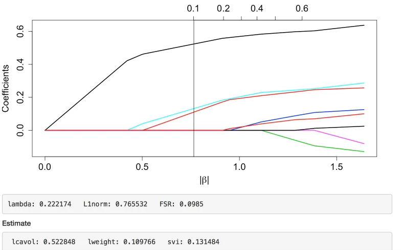
model exploration. Figure 2.1 shows an example of such a solution path using data from a

study on prostate cancer (Stamey et al., 1989); this figure is a screen capture from the software

provided in Chapter 3 that allows the analyst to mouse-over any point on the solution path

and examine the estimated coefficient values as well as the estimated false selection rate. In this

example, the selected point on the solution path corresponds to a model with three selected

variables, log cancer volume (lcavol); log weight (lweight); and seminal vesicale invasion (svi).

The estimated false selection rate corresponding to this model is 0.10 (additional details are

provided in Section 1.5.)

The proposed estimator of the false selection rate depends on the generation of

pseudo-variables that are conditionally independent of the response given the important pseudo-variables in

the model. As the true important variables are unknown in practice, our estimator consists

of three steps: (i) initial variable screening to estimate the set of important variables; (ii)

generation of pseudo-variables so that the covariance structure between the pseudo-variables

and those selected in the screening step mimics the covariance structure between the not-selected

and selected variables in the screening step; and (iii) fitting the penalized estimator and using

the proportion of selected pseudo-variables to construct an estimator of the false selection rate.

The proposed methodology is an example of a noise-variable or knock-off variable method. Such

methods have been applied to control the false selection rate in forward selection (Wu et al.,

2007) and for the Lasso (Barber et al., 2015; Barber and Cand`es, 2016). A primary contribution

(44)

(45)

λ(1), λ(2), . . . , λ(m)along the solution path that applies whenpn. When the proposed method

is used to tune the amount of penalization so as to achieve a target false selection rate, it provides

better empirical performance than alternatives in simulation experiments. Our theoretical and

methodological developments focus on a linear model estimated using the Lasso (Tibshirani,

1996) under a fixed design; however, simulation experiments illustrate broader applicability. To

facilitate the interactive model building, we have implemented the proposed methods in an R

package and a shiny web application both of which are described in the Chapter 3.

In Section 2.2, we establish notation, describe the proposed estimator, and state some of

its theoretical properties. In Section 2.3, we demonstrate the finite-sample performance of the

proposed method in a suite of simulation experiments. In Section 2.4, we illustrate application

of the proposed method using the data from prostate cancer study and leukemia cancer study.

Concluding remarks are made in Section 2.5.

2.2 Methods

2.2.1 Setup and notation

We consider data from a linear model under a fixed design. The observed data are{(Xi, Yi)}ni=1

and it is assumed thatYi =Xi|β0+i, where1, . . . , n iid

∼Normal(0, σ2), andβ0 = (β0,1, . . . , β0,p)|

∈_Rp_{. Define}

X= (X1, . . . , Xn)|∈Rn×p andY= (Y1, . . . , Yn)|. Given tuning parameterλ >0, the Lasso estimator of β0 is

b

βn(λ;Y,X) = arg min

β∈_Rp

  

1

2n||Y−Xβ||

2₊_λ p

X

j=1

|βj|

   .

DefineA0={j : β0,j 6= 0} to be the index set of nonzero coefficients in the true model and let

b An(λ) =

n

j : βb_n,j(λ;Y,X)6= 0 o

denote the active set atλ. For anyS⊆ {1, . . . , p}, writeXSto denote the design matrix composed of variables indexed byS; letSc_{denote the complement of}

S andN(S) the number of elements in S. Define Σ=n−1XA0,XAC

0

T

XA0,XAC

0

(46)

N nAb_n(λ) T

A0

o

; and Ub_n(λ) =N n

b

An(λ)\A0

o

. Thus, the false selection rate atλis pn(λ) =

EhUb_n(λ)/max n

b

In(λ) +Ub_n(λ),1 oi

.

2.2.2 Estimating the false selection rate

In this section, we provide a description of our estimator of the false selection rate for each model

along the Lasso solution path and provide theoretical justification; details of the implementation

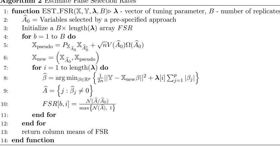
are deferred to the subsequent section. The proposed estimator is constructed in three stages:

(S1) apply screening to form a preliminary estimator of the set of nonzero coefficients,A0; (S2)

generate pseudo-variables that mimic the unimportant variables, i.e., those in Ac₀; and (S3) apply the Lasso to a dataset composed of the selected variables from the screening step and

the generated pseudo-variables; the proportion of pseudo-variables in the active set, Ab_n(λ), is the estimated false selection rate at tuning parameter valueλ.

Let r = rank(X) and for any square matrix, U, write U− to denote a pseudo-inverse.

For any non-empty subset S of {1, . . . , p}, define Q11(S) = n−1X|SXS, Q12(S) = n−1X|SXSc,

Q21(S) =n−1X|ScXS, Q22(S) = n−1X|ScXSc, and P

XS = XS(X |

SXS)−X|S. The estimator pbn(λ) of pn(λ) is constructed as follows.

Step 1 (Screening): For the full data (X,Y), apply a viable variable selection method to

construct a preliminary estimator,Ab₀_,n, of the set of nonzero coefficientsA₀. Let b

r0 denote

the rank of XAb0,n.

Step 2 (Pseudo-variable generation): Let Ω(Ab₀_,n)∈R(r−rb0)×{p−N(

b

A0,n)} _satisfy

Ω(Ab₀_,n)|Ω(Ab₀_,n) =Q₂₂(Ab₀_,n)−Q₂₁(Ab₀_,n)Q−₁₁(Ab₀_,n)Q₁₂(Ab₀_,n),

and letV(Ab₀_,n)∈Rn×(r−rb0) be any orthonormal matrix that is orthogonal to the column

space ofXAb0,n. Pseudo-variables have the form