ABSTRACT
BERRINGS, LAUREN M. State clustering in Markov Decision Processes with An Application in Information Sharing.
(Under the direction of Dr. Russell E. King and Dr. Thom J. Hodgson)
This research examines state clustering in Markov Decision processes, specifically addressing the problem referred to as Markov Decision process with restricted observations. The general problem is a special case of a Partially Observable Markov Decision process where the state space is partitioned into mutually exclusive sets representing the observable portion of the process. The goal is to find an optimal policy defined over the partition of the state space that minimizes (maximizes) some
performance objective. Algorithms presented to solve this problem for the infinite horizon undiscounted average cost case have largely been based on enumerative procedures. A heuristic solution procedure based on Howard’s (1960) policy iteration method is presented.
Applications of Markov decision processes with restricted observations exist in networks of queues, retrial queues, maintenance problems and queuing networks with server control. A new application area is proposed in the field of information sharing to measure the value of information sharing in a supply chain under optimal control. This is achieved by representing a model of full information sharing as a completely observable Markov Decision process (MDP), while no information sharing is represented as an MDP with restricted observations. Solution procedures are presented for the general Markov Decision process with restricted observations. Heuristic solutions are evaluated against the optimal solution obtained via total enumeration. Both random Markov Decision processes and information sharing problems are studied. The value of sharing
STATE CLUSTERING IN MARKOV DECISION PROCESSES WITH AN APPLICATION IN INFORMATION SHARING
by
LAUREN MARIE BERRINGS
A dissertation submitted to the Graduate Faculty of North Carolina State University
in partial fulfillment of the requirements for the Degree of
Doctor of Philosophy
INDUSTRIAL ENGINEERING
Raleigh
2004
APPROVED BY:
_________________________ ___________________________
Dr. R.E. King Dr. T.J. Hodgson
BIOGRAPHY
Lauren Marie (Berrings) Davis was born in Albany, New York on October 5, 1968 to Mary (Shearill) and Emanuel Berrings. She attended Rochester Institute of Technology where she received her Bachelor of Science in Computational Mathematics in 1991. Upon graduation, Lauren was awarded a GEM (Graduate Degrees for
Minorities in Engineering and Science) Fellowship and attended Rensselaer Polytechnic Institute in the fall of 1991. Her Master of Science in Industrial and Management Engineering was conferred in December 1992.
Lauren was offered a full-time software engineering position at IBM and relocated to North Carolina in 1993. Lauren has held many positions within the
Networking Hardware and Personal System Group divisions at IBM focusing on system integration and tools to support manufacturing. She currently works in the Integrated Supply Chain division where she has received three IBM Excellence awards for her role in the implementation of SAP across three manufacturing geographies.
ACKNOWLEDGMENTS
There are many people who helped to make this dream a reality. I thank Dr. Russell King for his guidance, support and patience throughout this process. I thank Dr. Thom Hodgson for the many challenges he unknowingly (or knowingly) gave me. Although they frustrated me at times, the challenges enabled me to grow in my
knowledge and approach to research. I can finally agree that my code can have errors. I thank Wenbin Wei, who is also doing research in this area, for the many ‘information sharing’ sessions we have held on the path to finishing our research.
The support my family and friends provided was invaluable. I thank my husband Tyrone for his love support and counsel. He has been an ad-hoc committee member challenging me to think outside the box. I thank my mom for all her prayers, words of wisdom and encouragement. I thank my Baptist Grove church family for keeping me in their prayers throughout this journey.
Table of Contents
LIST OF TABLES ... VII
LIST OF FIGURES ...VIII
CHAPTER 1 PROBLEM DESCRIPTION ... 1
1.1GENERAL DESCRIPTION... 1
1.2PROPOSED RESEARCH... 3
CHAPTER 2 LITERATURE REVIEW... 5
2.1INFORMATION SHARING... 5
2.1.1. Information Sharing Policies... 5
2.1.2 Models of information sharing... 6
2.1.2.1 Simulation Models... 9
2.1.2.2 Analytical Models... 10
2.1.2.3 Game Theoretic Models... 15
2.1.2.4 Mathematical Programming Models... 16
2.1.3 Value of sharing information ... 16
2.1.3.1 Benefits to the supplier under Dyadic Models... 17
2.1.3.2 Benefits to the Retailer under Dyadic Models... 18
2.1.3.3 Benefits to supply chain partners under Divergent models... 18
2.1.3.4 Benefits to supply chain under Network models... 20
2.1.4 Markov modeling approach to information sharing... 21
2.2MARKOV DECISION PROCESSES... 21
2.2.1 State clustering... 21
2.2.2 Markov processes with partial information... 23
2.2.3 Markov processes with restricted observations ... 24
2.2.3.1 General Problem... 24
2.2.3.2 Infinite Horizon Discounted Cost... 26
2.2.3.3 Finite Horizon Discounted Total Cost... 29
2.2.3.4 Infinite Horizon Average Cost... 31
2.2.4 Applicability of previous work to current problem... 33
CHAPTER 3 HEURISTIC FOR MDPS WITH RESTRICTED OBSERVATIONS35 3.1.BACKGROUND... 35
3.2.AN ALGORITHM FOR THE UNDISCOUNTED CASE... 35
3.2.1. Background and notation... 35
3.2.2 Model and Solution Method for ROMDP ... 36
3.2.4.1 Perturbation methods for steady state information vector... 49
3.3 EXPERIMENTAL RESULTS... 51
3.4CONCLUSIONS... 56
CHAPTER 4 SUPPLY CHAIN MODEL ... 57
4.1PROBLEM DESCRIPTION FOR INVENTORY INFORMATION SHARING... 57
4.2.1 Information sharing Models ... 59
4.2.2 Randomly Generated Models... 62
4.2.2.1 Solution by policy perturbation ... 62
4.2.2.2 Solution from Perturbations on information vector ... 65
4.3MEASURING THE VALUE OF INFORMATION SHARING... 70
CHAPTER 5 SENSITIVITY ANALYSIS ... 72
5.1OVERVIEW... 72
5.2SENSITIVITY ANALYSIS WITH POLICY PERTURBATION... 72
5.2.1 Experimental Design... 72
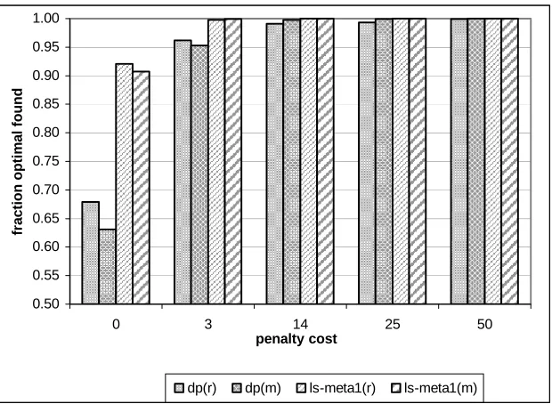
5.2.2 Penalty Cost Analysis ... 73
5.2.3 Retailer policy analysis... 78
5.2.4 Effect of initial policy... 79
5.2.2.5 Random restarts ... 81
5.3SENSITIVITY ANALYSIS WITH INFORMATION VECTOR PERTURBATION... 85
5.3.1 Overview ... 85
5.3.2 Sensitivity Analysis with epsilon ... 86
5.3.3 Termination Criteria based on problem size ... 88
5.4CONCLUSIONS... 92
CHAPTER 6 SUCCESSIVE APPROXIMATION APPROACH TO ROMDP ... 94
6.1BACKGROUND... 94
6.2DING PROCEDURE FOR UNDISCOUNTED MDP ... 94
6.3ADAPTATION FOR ROMDP... 96
6.3.1. Successive Approximation heuristic for ROMDP... 96
6.3.2 Periodic and Multi-Chain policies... 100
6.4EXPERIMENTATION... 102
6.4.1 Performance with respect to optimal solutions ... 103
6.4.2 Performance with respect to computation time ... 106
CHAPTER 7 A CASE FOR INFORMATION SHARING... 108
7.1PROBLEM DESCRIPTION... 108
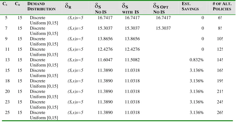
7.2DEMAND EFFECT ON VALUE OF INFORMATION SHARING... 110
7.2.1 Design of experiment ... 110
7.2.2 Results ... 111
7.3CAPACITY EFFECT ON VALUE OF INFORMATION SHARING... 113
7.3.1 Design of Experiment... 113
7.3.2 Results ... 113
7.4RETAILER POLICY EFFECT ON VALUE OF INFORMATION SHARING... 121
7.4.1 Design of Experiment... 121
7.4.2 Results ... 121
7.7 CONCLUSIONS... 130
CHAPTER 8 CONCLUSIONS AND FUTURE WORK ... 133
8.1CONCLUSIONS... 133
8.2ADDITIONAL RESEARCH... 133
8.3STOCHASTIC GAMES... 134
REFERENCES... 135
APPENDIX A INFORMATION SHARING CHARTS... 139
List of Tables
TABLE 2.1INFORMATION SHARING RESEARCH BY STRUCTURE AND MODEL... 7
TABLE 2.2RESEARCH SUMMARY BY METHOD... 25
TABLE 2.3RESEARCH SUMMARY BY AUTHOR... 25
TABLE 3.1AVERAGE EXECUTION TIME IN CPU SECONDS... 53
TABLE 3.2AVERAGE EXECUTION TIME IN CPU SECONDS... 56
TABLE 4.1.POLICIES FOR INVENTORY SHARING/PERFECT SUPPLIER/LOST SALES... 59
TABLE 4.2.INVENTORY SHARING/PERFECT SUPPLIER/LOST SALES –GAIN... 60
TABLE 4.3.CAPACITY INFLUENCE ON INVENTORY SHARING/PERFECT SUPPLIER/LOST SALES INSTANCES... 61
TABLE 4.4. INFORMATION SHARING SUMMARY FOR BINOMIAL DEMAND (S,S) PROBLEM. 71 TABLE 5.1SUPPLY CHAIN PROBLEM PARAMETERS... 82
TABLE 5.2RANDOM RESTART RESULTS FOR LARGER PROBLEM SIZES... 85
TABLE 5.3INFORMATION VECOTR PERTURBATION PERFORMANCE... 89
TABLE 5.4TOTAL ENUMERATION EXECUTION TIME... 89
TABLE 5.5RANDOM RESTART WITH INFORMATION VECTOR PERTURBATION RESULTS FOR (6,6)PROBLEM... 90
TABLE 5.6RANDOM RESTART WITH INFORMATION VECTOR PERTURBATION RESULTS FOR (5,5)PROBLEM... 90
TABLE 5.7RANDOM RESTART WITH INFORMATION VECTOR PERTURBATION RESULTS FOR (4,4) AND (3,3)PROBLEMS... 91
TABLE 5.8EXECUTION TIME FOR ROMDPHEURISTIC AND TOTAL ENUMERATION... 92
TABLE 6.1RESULTS FOR RANDOMIZED DISCRETE DISTRIBUTION AND BASE STOCK (CR) POLICY... 104
TABLE 6.2RESULTS FOR BINOMIAL DEMAND DISTRIBUTION AND (S,S)RETAILER POLICY ... 104
List of Figures
FIGURE 2.1DYADIC SUPPLY CHAIN... 7
FIGURE 2.2SERIAL SUPPLY CHAIN... 8
FIGURE 2.3DIVERGENT SUPPLY CHAIN... 8
FIGURE 2.4CONVERGENT SUPPLY CHAIN... 8
FIGURE 2.5NETWORK SUPPLY CHAIN... 8
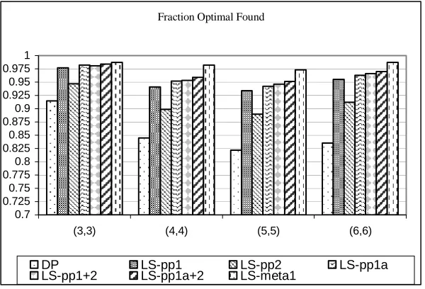
FIGURE 3.1FRACTION OPTIMAL SOLUTIONS FOUND OVER 1000 INSTANCES... 52
FIGURE 3.2AVERAGE RELATIVE ERROR FOR NON-OPTIMAL SOLUTIONS... 52
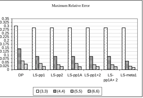
FIGURE 3.3MAXIMUM RELATIVE ERROR FOR NON-OPTIMAL SOLUTIONS... 53
FIGURE 3.4FRACTION OPTIMAL FOUND (3X3) ... 54
FIGURE 3.5FRACTION OPTIMAL FOUND (4X4) ... 54
FIGURE 3.6FRACTION OPTIMAL FOUND (5X5) ... 55
FIGURE 3.7FRACTION OPTIMAL FOUND (6X6) ... 55
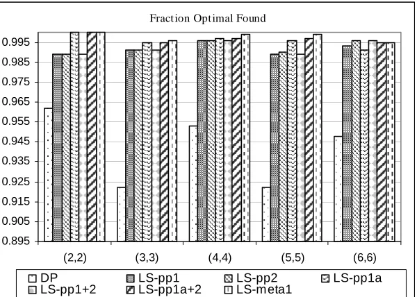
FIGURE 4.1FRACTION OPTIMAL FOUND –RANDOMIZED DISCRETE DISTRIBUTION... 63
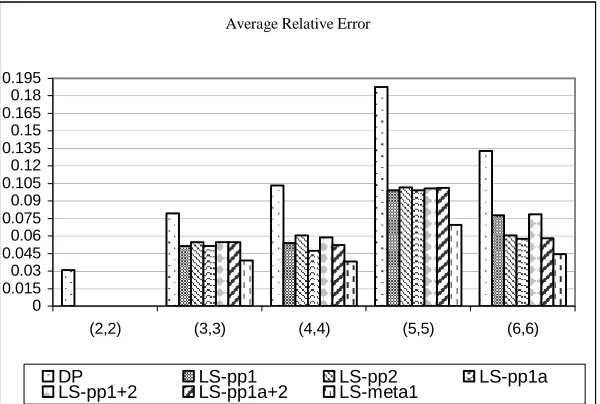
FIGURE 4.2AVERAGE RELATIVE ERROR –RANDOMIZED DISCRETE DISTRIBUTION... 63
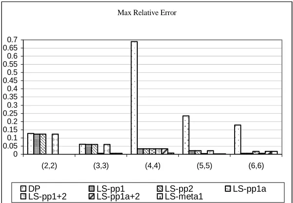
FIGURE 4.3MAXIMUM RELATIVE ERROR –RANDOMIZED DISCRETE DISTRIBUTION... 64
FIGURE 4.4FRACTION OPTIMAL FOUND -BINOMIAL DEMAND DISTRIBUTION... 64
FIGURE 4.5AVERAGE RELATIVE ERROR -BINOMIAL DEMAND DISTRIBUTION... 65
FIGURE 4.6MAXIMUM RELATIVE ERROR -BINOMIAL DEMAND DISTRIBUTION... 65
FIGURE 4.7FRACTION OPTIMAL FOUND –RANDOMIZED DISCRETE DISTRIBUTION (2,2) ... 66
FIGURE 4.8FRACTION OPTIMAL FOUND –RANDOMIZED DISCRETE DISTRIBUTION (3,3).... 67
FIGURE 4.9FRACTION OPTIMAL FOUND –RANDOMIZED DISCRETE DISTRIBUTION (4,4).... 67
FIGURE 4.10FRACTION OPTIMAL FOUND –RANDOMIZED DISCRETE DISTRIBUTION (5,5).. 67
FIGURE 4.11FRACTION OPTIMAL FOUND –RANDOMIZED DISCRETE DISTRIBUTION (6,6).. 68
FIGURE 4.12FRACTION OPTIMAL FOUND -BINOMIAL DEMAND DISTRIBUTION (3,3) ... 68
FIGURE 4.13FRACTION OPTIMAL FOUND -BINOMIAL DEMAND DISTRIBUTION (4,4) ... 69
FIGURE 4.14FRACTION OPTIMAL FOUND -BINOMIAL DEMAND DISTRIBUTION (5,5) ... 69
FIGURE 4.15FRACTION OPTIMAL FOUND -BINOMIAL DEMAND DISTRIBUTION (6,6) ... 70
FIGURE 5.2RANDOMLY GENERATED DISCRETE DISTRIBUTION (S,S)POLICY FOR RETAILER
... 74
FIGURE 5.3BINOMIAL DEMAND,(S,S)POLICY FOR RETAILER... 75
FIGURE 5.4RANDOMLY GENERATED DISCRETE DISTRIBUTION,BASE STOCK POLICY, PENALTY COST OF 0... 75
FIGURE 5.5RANDOMLY GENERATED DISCRETE DISTRIBUTION,BASE STOCK POLICY, PENALTY COST OF 50... 76
FIGURE 5.6BINOMIAL DEMAND,(S,S)POLICY, PENALTY COST OF 3 ... 76
FIGURE 5.7BINOMIAL DEMAND,(S,S)POLICY, PENALTY COST OF 3 ... 77
FIGURE 5.8BINOMIAL DEMAND,(S,S)POLICY, PENALTY COST OF 3 ... 77
FIGURE 5.9POLICY ITERATION PERFORMANCE (NO PERTURBATION)... 78
FIGURE 5.10POLICY ITERATION -PERTURBATION PERFORMANCE... 78
FIGURE 5.11RANDOMIZED DISCRETE DISTRIBUTION,BASE STOCK POLICY FOR RETAILER ... 80
FIGURE 5.12RANDOMIZED DISCRETE DISTRIBUTION,(S,S)POLICY FOR RETAILER... 80
FIGURE 5.13BINOMIAL DEMAND DISTRIBUTION,(S,S)POLICY FOR RETAILER... 81
FIGURE 5.7FRACTION OPTIMAL FOUND FOR PROBLEM P1 ... 82
FIGURE 5.8MAXIMUM RELATIVE ERROR FOR PROBLEM P1 ... 82
FIGURE 5.16FRACTION OPTIMAL FOUND FOR PROBLEM P2 ... 83
FIGURE 5.9MAXIMUM RELATIVE ERROR FOR PROBLEM P2 ... 83
FIGURE 5.18FRACTION OPTIMAL FOUND FOR PROBLEM P3 ... 84
FIGURE 5.19MAXIMUM RELATIVE ERROR FOR PROBLEM P3 ... 84
FIGURE 5.20FRACTION OPTIMAL FOUND -EPSILON CHANGING... 87
FIGURE 5.21FRACTION OPTIMAL FOUND FOR (4,4)PROBLEM... 87
FIGURE 5.22FRACTION OPTIMAL FOUND FOR (5,5)PROBLEM... 88
FIGURE 5.23FRACTION OPTIMAL FOUND (6,6)PROBLEM... 88
FIGURE 7.1RELATIVE VOI VERSUS DEMAND... 111
FIGURE 7.5EXPECTED SUPPLIER PRODUCTION OUTPUT FOR BINOMIAL DEMAND PROBLEM
... 116
FIGURE 7.6EXPECTED RETAILER LOST SALES AND SUPPLIER PRODUCTION FOR BINOMIAL DEMAND PROBLEM... 116
FIGURE 7.7VALUE OF (S)AS A FUNCTION OF SUPPLIER CAPACITY... 117
FIGURE 7.8MODIFIED STATE DEPENDENT ECHELON BASE STOCK POLICY... 118
FIGURE 7.9MODIFIED STATE DEPENDENT ECHELON BASE STOCK POLICY FOR RECURRENT STATES (BINOMIAL DEMAND DISTRIBUTION) ... 119
FIGURE 7.10RELATIVE VOI FOR BINOMIAL DISTRIBUTION... 120
FIGURE 7.11RELATIVE VOI FOR BINOMIAL DEMAND... 122
FIGURE 7.12RELATIVE VOI FOR UNIFORM DEMAND... 122
FIGURE 7.13RELATIVE VOI FOR POISSON DEMAND... 122
FIGURE 7.14EXPECTED LOST SALES WITH (S,S) AND BASE STOCK... 123
FIGURE 7.15AVERAGE PER PERIOD COSTS WITH (S,S) AND BASE STOCK... 123
FIGURE 7.16EXPECTED SUPPLIER PRODUCTION AS A FUNCTION OF SUPPLIER CAPACITY ... 124
FIGURE 7.17RETAILER STEADY STATE INVENTORY POSITION EACH REVIEW PERIOD.... 126
FIGURE 7.18RETAILER STEADY STATE ORDER DISTRIBUTION... 126
FIGURE 7.19ORDER DISTRIBUTION WHEN DEMAND IS B(20,0.75) AND RETAILER POLICY IS BASE STOCK CR... 128
FIGURE 7.20ORDER DISTRIBUTION WHEN DEMAND IS B(20,0.75) AND RETAILER POLICY IS (S,S) ... 128
FIGURE 7.21RELATIVE VOI AS FUNCTION OF VARIABLE ORDER COST,SUPPLIER CAPACITY=13, ... 129
Chapter 1 Problem Description
1.1 General Description
This research examines state clustering in Markov Decision processes, specifically addressing the problem referred to as Markov Decision process with restricted observations. The general problem is a special case of a Partially Observable Markov Decision process where the state space is partitioned into mutually exclusive sets representing some observable portion of the process. The goal is to find an optimal policy defined over the observable portion of the state space that minimizes (maximizes) some performance objective. The policy obtained is referred to as an implementable policy. The initial motivation for work on state clustering derived from the need to reduce the dimensionality of the state space for large-scale multi-stage inventory problems, thus enabling solutions of these problems to be obtained in a reasonable
amount of time on a computer. We are motivated to continue work in this area due to our interest in its applicability for measuring the value of information sharing in a supply chain. Howard(1971), Kemney and Snell(1960), and Dietz(1983) provide conditions under which a cluster state can be created. Observability constraints for the MDP were added to reflect systems in which the entire state space is not visible to the decision-maker. In this situation, new policies are required to determine optimal control based on what could be observed and implemented by a decision-maker in a real time system.
Algorithms developed to address this problem have covered infinite and finite time horizons as well as discounted and undiscounted costs. Serin and Avsar (1997) studied the finite horizon discounted cost case and proposed an algorithm that finds a global deterministic optimal policy. This research will cover the infinite horizon
Applications of Markov decision processes with restricted observations exist in networks of queues, retrial queues, maintenance problems and queuing networks with server control (Hordijk and Loeve (1994),Serin and Avsar(1997)). A new application area is proposed in the field of information sharing. Specifically, the algorithm can be used to measure the value of information sharing in a supply chain under various supply chain structures. Information sharing entails sharing key pieces of operational data between supply chain partners to improve performance. Supply chain partners can share any combination of inventory, demand, sales forecast, and production or delivery
schedule information. Supply chain members consist of suppliers, manufacturing sites, distribution centers, retailers and consumers which can be contained within one company or consist of several external parties whose resources are combined into an end product for the consumer. By sharing information, it is believed that the negative impact of uncertainty (demand, production, etc.) on the supply chain performance can be minimized.
Several applications of information sharing have been incorporated into the logistics operations of many companies, reportedly improving the efficiency of the members in the supply chain. Lee and Whang (2000) provide a thorough description of the levels of information sharing and the companies using such programs to improve supply chain performance. Several papers have been published quantifying the value of information sharing to the supply chain and characterizing the conditions in which it is most
beneficial. These papers examine impact of sharing inventory, point of sale (POS) data, sales forecast, and production and delivery schedule data in several supply chain
structures. The value of the information is measured by developing a model that compares the supply chain costs and order decisions with and without the additional information, and analyzing key performance measures such as average inventory, order quantity, backorders, and per period costs. The following assumptions are commonly made in these models.
1. Two-stage supply chains with a single supplier and retailer or a single supplier and multiple retailers
2. Capacitated supplier
4. Order-up-to or (s, S) inventory control policy employed by retailer and/or supplier 5. Periodic-review inventory management
For these models, optimal or near-optimal inventory control or supply allocation policies are determined and the cost savings associated with the various levels of
information sharing compared. The methodology used to determine the optimal policies and cost benefits have varied. A gradient-based simulation procedure known as
infinitesimal perturbation analysis is used by Zhao and Simchi-Levi(2002), Gavirneni (2001,2002), and Gavirneni et al.(1999). Zhao et al. (2002a) uses a simulation model to quantify the value of information sharing. Analytical models incorporating information flow into inventory control models are employed by Cachon and Fisher (2002), Lee et al. (2000), Yu et al. (2001) and Raghunathan (2001).
In this research, Markov Decision models are developed to determine the gain and optimal control policies, which are used to determine the associated savings with and without information sharing. A Markov model is a natural way to represent a system where information is shared. Based on the supply chain structure being used, the definition of the state space indicates the available information known to the decision-maker at any point in time. A completely observable MDP is used to model the
information sharing case. The case of no or limited information sharing is modeled as a Markov Decision Process with restricted observations and solved via the algorithm proposed in this research.
1.2 Proposed Research
Chapter 2 contains a summary of the approaches taken to study the value of information sharing and the results gleaned from those models. Solution procedures and conditions for state clustering in Markov decision processes are also presented.
A new heuristic for solving the MDP with restricted observations (ROMDP) is outlined in chapter 3. Initial results are presented in chapter 4 for a simple two-stage supply chain sharing demand and inventory information. Results are also given for a randomly
Chapter 2 Literature Review
2.1 Information sharing
2.1.1. Information Sharing Policies
Information sharing is the action of taking imperfect information and making it ‘nearly’ perfect. This action between supply chain members involves sharing one or more characteristics about the demand or manufacturing process. This additional information enables the recipient to provide better service in the form of better supply commitments, fewer lost sales or backorders, or better management of demand
fluctuations and thus improved reliability. Some of the characteristics that can be shared are the actual demand realized during the period, the demand forecast, inventory position or inventory control policy. The parameters that define an information sharing policy are typically the type of information being shared and the direction of information flow between the participating supply chain members.
There is no standard terminology or nomenclature to characterize information sharing policies. The definition of the policy structure is usually subject to the
researcher. However, the no information sharing policy is commonly recognized as the historical method of communication between suppliers and retailers. Under this policy, information about the retailer’s demand or ordering policy is unknown. The only
information the supplier receives is in the form of orders from the retailer. Therefore, the retailer’s process is like a ‘black box’ to the supplier. Gavirneni(2001) uses the term partial information sharing to denote a policy in which the demand distribution and the parameters of the inventory control policy used by the retailer are known.
sharing policies being developed, the direction of information flow can continue to be upstream. The potential amount of information flowing upstream is now greater. For example, the supplier can have access to the retailer’s inventory data in addition to point of sale data. The information can also flow downstream from the supplier to the retailer. An example of this type of policy may be in the form of consignment, where the retailer has access the supplier’s inventory and is only charged based on the amount they extract from inventory. Bi-directional type of information flow can also occur between the supply chain members. Cachon and Fisher (2000) model this type of policy with 1 supplier and N retailers sharing inventory data between all members in the supply chain retailer to retailer as well as supplier to retailer. This type of supply chain configuration may be seen between regional distribution centers, where stock can be reallocated between the warehouses by a single controlling entity.
2.1.2 Models of information sharing
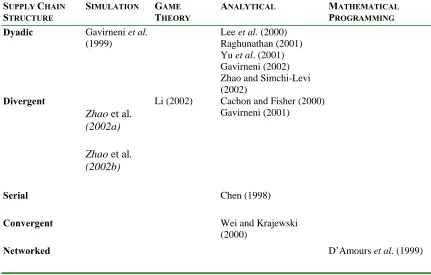
suppliers and multiple stages in the manufacturing process depending upon the structure of the end item being produced. Finally, a network structure is a complex supply chain combining elements from the divergent and convergent structure. Refer to figure 2.5 for an example of a network supply chain structure. The bulk of the research consists of analytical models of dyadic and divergent structures. Selected papers relevant to this research are discussed in the following sections and summarized below in table 2.1 by supply chain structure and modeling approach. Some of the models are included in the hierarchical summary by Huang et al. (2003) and some are new contributions since the publication of his work.
Table 2.1 Information Sharing Research By Structure and Model
SUPPLY CHAIN
STRUCTURE
SIMULATION GAME
THEORY
ANALYTICAL MATHEMATICAL
PROGRAMMING
Dyadic Gavirneni et al. (1999)
Lee et al. (2000) Raghunathan (2001) Yu et al. (2001) Gavirneni (2002) Zhao and Simchi-Levi (2002)
Divergent
Zhao et al. (2002a) Zhao et al. (2002b)
Li (2002) Cachon and Fisher (2000) Gavirneni (2001)
Serial Chen (1998)
Convergent Wei and Krajewski
(2000)
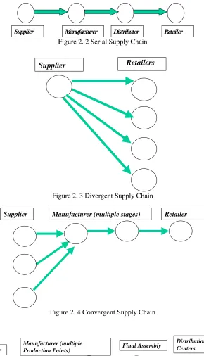
Supplier Manufacturer Distributor Retailer
Figure 2. 2 Serial Supply Chain
Supplier Retailers
Figure 2. 3 Divergent Supply Chain
Supplier Manufacturer (multiple stages) Retailer
Figure 2. 4 Convergent Supply Chain
Supplier Final Assembly
Manufacturer (multiple Production Points)
Distribution Centers
2.1.2.1 Simulation Models
Zhao et al. (2002a) use a simulation model to study the value of sharing sales forecast information in a divergent supply chain system consisting of a single capacitated supplier and four retailers. Transportation lead-time is one period, implying that a single truck can deliver the required shipment to each retailer during that time. The retailers use an EOQ inventory policy and the supplier uses single-item capacitated lot-sizing to plan its production activities. Backorders are allowed at the supplier and retailers. The cost savings to the supply chain are evaluated by varying retailer’s demand pattern, supplier capacity, information sharing level, and order coordination. Ordering coordination (OC) refers to negotiating longer lead-time for parts by placing orders with the supplier in advance. Conditions by which the retailer and/or supplier benefit are characterized by examining the decisions made by the supplier under each information sharing policy and quantifying the resulting affect on the performance of the supply chain. When no
information is shared (NIS), the supplier’s production decisions are based on the orders received from the retailer. When demand forecast data is shared (DIS), the supplier’s production decisions are based on the retailer’s order and the forecasted demand. The supplier’s decision under the policy of sharing planned orders (OIS) is based on the retailer’s order and future planned orders generated as a result of the retailer demand forecast. Using the same model assumptions described above, Zhao et al. (2002b) also study the impact of forecast model selection on the value of information sharing. Several forecasting methods are evaluated ranging from simple models with poor level of
order quantity either in full from the supplier or in part from the supplier and part from somewhere else. Infinitesimal perturbation analysis is used to determine the optimal order up to level and total costs incurred by the supplier at each level of information sharing. Simulation is performed to measure the value of information sharing under the optimal policies. The interaction between information sharing and different measures of performance, such as inventory and capacity, are also examined by varying demand distributions, levels of capacity, and inventory control parameters. The three possible policies associated with information sharing are no sharing, partial sharing and full sharing. Under a policy of no information sharing, information about the retailer demand or ordering policy is not known. The supplier demand and subsequent control policy is based on the order quantity. With a partial information sharing policy, the demand distribution and the parameters of the inventory control policy are known. With this information, the supplier can determine the probability of an order being generated at the end of the period and the CDF of the order size. Under a policy of full information sharing, the demand distribution, (s, S) policy parameters, and immediate information about demand are known. Again, the CDF of the order size and probability an order is placed can be determined. The results indicate increasing levels of information flow, in all cases, reduces the supplier’s costs. The degree of the savings depends on the capacity available, the end-item demand variance, and the retailer order quantity (S-s).
2.1.2.2 Analytical Models
Lee et al. (2000) develop a base stock model to investigate the impact of sharing point of sale data in a two-stage supply chain consisting of a single retailer and a single manufacturer. The retailer demand follows a first order autoregressive (AR(1)) process and both the retailer and manufacturer employ an order-up to inventory control policy. The ordering cost is assumed to be zero and the manufacturer knows the demand follows an AR(1) process. When no information sharing (NIS) occurs, the manufacturer’s order decision is based solely on the demand as a function of the retailer’s order quantity at the end of the period. Under information sharing (IS), the manufacturer receives the order quantity and the retailer’s demand at the end of the time period. Based on the
cost as a function of the forecast demand are developed. The variance of the forecast demand is smaller when information sharing occurs and thus the supplier experiences inventory reduction. The expressions obtained analytically are verified with a simulation study.
Raghunathan (2001) uses the model developed by Lee et al. (2000) to demonstrate the value reported is insignificant. The key difference between the two models is that under a policy of no information sharing, Raghunathan assumes the retailer order history is used to forecast future orders while Lee et al. (2000) assume the
manufacturer uses only the most recent order from the retailer to forecast future orders. Ragunathan reports the value of information sharing decreases monotonically with each time period, converging to zero in the limit. He suggests that information sharing of demand data can be valuable to the manufacturer if none of the demand parameters can be inferred from the order history.
Yu et al. (2001) analyze the value of sharing point of sale and inventory information in a two-stage supply chain. They develop a discounted cost-minimizing inventory model that is used to derive the optimal inventory policy for the members in the supply chain. The resulting policy is then used to analyze the average inventory level and expected costs under the different levels of information sharing. Both supply chain partners use an (s, S) inventory control policy with periodic review. Excess demand is backlogged and each supply chain member incurs holding, penalty, and order costs during each period. The information sharing and order coordination policies evaluated are no sharing, coordinated control and centralized control. When no information is shared, the inventories at the different sites are controlled independently. Under a policy of coordinated control, the retailer's customer demand is shared with the manufacturer. The manufacturer’s order decision is based on both the customer demand the retailer's order information. When complete information and coordination occurs (centralized control), the customer demand and retailer inventory information is shared. The
linear holding costs at every stage and linear backorder costs at the first stage. Production lead times are constant between stages and it is assumed that a reorder point /order quantity policy is used at all stages. The order quantities at each stage are fixed and the reorder point at each stage is the decision variable. The value of centralized demand information is measured as the relative cost difference associated with implementing an echelon based batch reorder point policy and installation based batch reorder point policy. Echelon based policies represent the optimal replenishment strategy when centralized demand information is used, while installation based policies represent the optimal replenishment strategy when local demand information is used. The optimal echelon reorder point policies are determined by decomposing the problem into single-stage models which are solved sequentially, similar to the approach developed by Clark and Scarf (1960). The installation based reorder point policies are determined using a bounded search procedure.
Cachon and Fisher (2000) develop an analytical model to examine the value of inventory information sharing on a supplier’s order and allocation decisions in a periodic review system. The supply chain structure consists of N identical retailers and a single infinite capacity supplier. Batch reorder point policies are used by the retailer and the supplier when no information is shared and by the retailer only when information is shared. The supplier’s optimal policy and allocation decision are determined from the shared information. Under traditional information sharing, the supplier receives only the order quantity and allocates available inventory based on a batch priority scheme. In full information sharing, the supplier knows the inventory level at all retailers, and allocates supply in a manner that balances the retailer’s inventory levels across the system. The additional shared information is used to determine the optimal policy and allocation decision for the supplier. Simulation is used to approximate the optimal policy and estimate the expected per period supply chain costs associated with the full information sharing policy. The optimal policy and per period costs under the traditional case is determined via a search over all feasible policies.
capacitated; there is no batch size for reordering; and the benefits of information sharing are computed by comparing optimal policies. The model of Cachon and Fisher (2000) uses at least one non-optimal policy in computing the benefits. When no information is shared the orders are filled in a predetermined sequence. When partial information is shared, retailer demand and inventory levels between the supplier and retailers are known. Inventory is allocated amongst the retailers in a manner that ensures retailers with lower inventories receive larger shipments. In a system with complete information sharing, inventory levels are shared between all members in the supply chain, supplier to retailer and retailer-to-retailer. Retailers with very high inventory levels are willing to give up inventory and face higher penalty costs in order to help those retailers with very low inventory levels. As a result, the supplier can move inventory between retailers to satisfy other retailers order quantities. Demand not satisfied by the supplier is lost and demand not satisfied by the retailers is backlogged. Infinitesimal Perturbation Analysis is used to compute the optimal order up to level and per period retailer holding and penalty costs for each model. When no information is shared, each retailer has its own order up to level, while in the other models each retailer has the same order up to level.
Gavirneni (2002) examines the effect of information sharing when operating policies used by the retailer are changed to make better use of the information flows within the supply chain. Two models consisting of demand and cost information sharing between a supplier and retailer are evaluated. In the first model (Model 1), the retailer uses his optimal (s,S) inventory control policy and the optimal order up to policy for the supplier is determined using IPA. The supplier knows the cumulative demand at the retailer since the last order occurred and therefore can estimate, in each period, the
incurred as a result of producing earlier in anticipation of demand. The cost function is formulated as a stochastic dynamic program and IPA is used to compute the optimal order up to levels.
Zhao and Simchi-Levi (2002) also use infinitesimal perturbation analysis (IPA) to quantify the cost savings to the supplier when demand information is shared in a two-stage production inventory system. The information sharing problem is modeled as a Markov decision process to prove that a cyclic order up to policy for the supplier is optimal and has a finite steady state average cost for the discounted and average cost criteria. However, infinitesimal perturbation analysis is used to compute the optimal policy and compare the resulting costs under the different information sharing levels. The retailer uses a periodic review system with an order-up-to inventory policy. The model also examines the effect of frequency and timing of information shared on the costs incurred by the supplier. The point in time where demand is shared and production decisions can be made but no retailer order is placed is referred to as an Information Period. The time at which retailer orders are placed is referred to as an Ordering Period. Several information periods exist between ordering periods. Under a policy of no
information sharing, demand information is received at the order interval. When information sharing is employed, the retailer shares point of sale data for each information period and places orders during their ordering period. The model of no information sharing is the information sharing model with zero information periods.
integration, the manufacturer considers the flexibility capability of all tier 1 suppliers when determining his scheduling policy. Under critical path, only the capabilities of the critical path suppliers are used in the determination of the best policy. Total integration considers the capability for all members in the supply chain. Flexibility capabililty is a numerical measure describing the ability of the members to adapt to schedule changes by the manufacturer. A stochastic cost model is used to determine the best policy that minimizes the total costs associated with schedule changes, shipping costs, material and inventories. Results indicate that the ranking of costs associated with schedule integration is total sharing < critical path < tier-1 < myopic. Schedule change costs are a primary driver of the optimal policies and the cost ranking is unaffected by demand variation. Based on analysis of the results, Wei and Krajewski (2000) suggest that it is more cost effective for the manufacturer to focus on integration with suppliers in the critical path.
2.1.2.3 Game Theoretic Models
2.1.2.4 Mathematical Programming Models
D’Amours et al. (1999) use a network flow model to examine the impact of price and capacity information sharing in a networked manufacturing environment. The supply chain structure consists of a single (networking) firm with partnerships between several manufacturing, transportation and storage firms. The networking firm must choose and schedule the order among the available firms in order to satisfy the customer order. The information policies are expressed in terms of the bidding protocols representing
information transferred between the networking firm and the contracting firms. In supplier–type bids, information transferred in the bid is publicly known price and time packages. In customizing-type bids, price and time packages are customized based on the needs of the networking firm. The networking firm shares capacity and time requirements. The contracting firms share price-time package information based on needs of the networking firms. The package represents a maximum set of alternatives that can be constructed to support the order. In webbing-type bids, information shared from contracting firms to networking firms is day-to-day operating characteristics, production capability, capacity requirements and pricing functions. From this
information, the networking firm generates their own set of bid alternatives. All possible bids within each type are formulated as a network flow problem. The objective is to configure and schedule a virtual manufacturing and logistics network to satisfy delivery and quantity requirements of customer.
2.1.3 Value of sharing information
in reduced inventories and reduced costs. A summary of the results is presented by supply chain structure and reference point.
2.1.3.1 Benefits to the supplier under Dyadic Models
Lee et al. (2000) show the inventory reduction and cost reduction with
information sharing is significant only when the demand is highly correlated over time, highly variable or when the lead-time is long. However, Ragunathan (2001) shows, for the same model, that information sharing decreases monotonically with each time period when the supplier uses a better forecasting method under no information sharing. Only when the demand parameters cannot be inferred from the order history, is information sharing significant. These two papers demonstrate how results vary based on the
integration of information into the decision process. Gavirneni et al. (1999) also examine the effect demand variance has on possible savings with information sharing. They varied the variance of Normal, Uniform, and Erlang distributions while keeping the mean value common. For each distribution, the percentage savings increased and then decreased as the coefficient of variation was decreased. They concluded the variance of the retailer’s demand distribution limits the cost benefits that can be achieved with information sharing. When the demand variance is high, the reduction in uncertainty due to the additional information is insignificant from a cost perspective. At moderate values of demand variance, information sharing appears to be most beneficial.
ordering period. When capacity is tight, the cost is less sensitive to the timing of information sharing.
With respect to the inventory control parameters of an (s,S) policy, Gavirneni et al. (1999) show the percentage savings between partial information sharing and full information sharing has no significant differences. Both policies demonstrate the information is less beneficial at extreme values of the order quantity (S-s). The authors attribute this behavior to the fact that the extreme order quantities reduce the benefit of sharing information. When (S-s)is large, the supplier has to build up inventory in anticipation for a large order. When (S-s)is small, the demand information is passed to the supplier almost every period, thus reducing the benefit of sharing demand
information.
Yu et al. (2001) use their model to study the expected per period costs. The results show that suppliers benefit under each increasing level of information sharing; no information sharing, coordinated control (demand is shared) and centralized control (demand and inventory is shared). As information is shared, the inventory levels at the manufacturer decrease, resulting in smaller expected per period cost.
2.1.3.2 Benefits to the Retailer under Dyadic Models
Yu et al. (2001) examine the affect of information sharing on the retailer as well as the supplier. The key results indicate there is no benefit to the retailer by sharing their customer demand with the manufacturer. The average inventory and expected costs between coordinated control (demand information is shared) and no information sharing remain the same. Under centralized control, where demand and inventory information is shared, the retailer realizes performance improvement because the retailer's lead-time is reduced due to the improvement in the manufacturer’s reliability as a result of using VMI. Since the supplier receives most of the benefit from information sharing, the authors suggest some incentive should be offered to induce the retailer to share their demand information.
2.1.3.3 Benefits to supply chain partners under Divergent models
possible. However, the expected profit for the retailers is less when they share information. The incremental loss from sharing gets smaller as more retailers share information. So the resulting equilibrium strategy is to not share information. From a total supply chain perspective, profit is larger with information sharing when the information each retailer has is informative in a statistical sense or when there is a sufficiently large number of retailers. Li also suggests the manufacturer should provide incentives to the retailer to share information and discusses a contract signing game where retailers are compensated by some fixed amount. Boundary conditions are provided for the compensation value.
Zhao et al. (2002a,) also study the value of information sharing from the supplier, retailer and total supply chain perspective. The supplier is usually the benefactor in all cases of increased information sharing and ordering coordination. The retailer benefits only when all retailers face identical demands with decreasing trend and the supplier’s capacity utilization with respect to capacity needed to meet the demand is high (85% or 95%). When order coordination is high and demand is different for each retailer, the supplier’s service level increases but at the expense of the retailer and the supply chain. High order coordination implies the lead-time between orders increase. Retailers are placing their orders several periods in advance. When this occurs, retailer’s forecast errors increase, resulting in deteriorated service levels and increased backorder costs. Therefore, total costs for the retailers and the supply chain increase. Similar results are reported when studying the impact of forecast model selection on the value of
information sharing. (Zhao et al. (2002b)). In addition, the value of information sharing is greatest when the forecast accuracy, measured in terms of standard deviation of the forecast error, is high.
one-to-view and finds that information is more beneficial at lower capacities and higher penalty costs, when comparing no information sharing to demand and inventory level sharing. At lower capacities, the supplier is not able to meet all of the retailers’ demands and
information enables him to allocate capacity better. When capacity is high, the demand can be satisfied for all retailers and thus information is not beneficial. Gavirneni (2001) measures capacity as a ratio of supplier’s capacity to the retailer’s mean demand. This contradicts results discussed earlier in Gavirneni et al. (1999) for a dyadic supply chain structure. However, these results demonstrate how the affect of capacity on the value of information sharing differs under different supply chain structures, information sharing policy, measures of capacity and model assumptions.
Gavirneni (2001) also finds information to be less beneficial between no
information and some cooperation (demand and inventory sharing) when demand is not highly variable. Using the Erlang and Exponential distributions, results show as variance decreases, the percentage benefit decreases. He also studies the affect the number of retailers in the distribution chain has on the value of information. In this case, as the number of retailers increase, the benefit from information sharing decrease.
Cachon and Fisher (2000) look at total supply chain costs to quantify the benefits of information sharing. Their results indicate full information sharing provide an average benefit of 2.2% over the traditional information sharing case. The authors also conclude that higher cost savings can be achieved through lead-time reduction and smaller order batch sizes. Lead time reduction results in an average cost savings of 21% while batch size reduction results in an average cost savings of 22%.
2.1.3.4 Benefits to supply chain under Network models
scheduling comes at the cost of more complexity. The complexity is in terms of the number of manufacturing and logistics units selected to schedule the order.
2.1.4 Markov modeling approach to information sharing
In all of the papers studying information sharing, no one has examined this problem from the perspective of steady state optimal control. A Markov model is a natural way to represent a system where information is shared. Based on the supply chain structure being used, the definition of the state space indicates the available information known to the decision maker at any point in time. By collapsing the state space, you restrict the information known and affect the policy chosen. Both models yield the steady-state optimal policy and gain, which provide a consistent and equivalent measure of performance between the two systems. There are several advantages to studying information sharing as a Markov Decision process. There is a single model that yields the optimal policy for the decision maker along with one consistent measure of performance: the gain. With simulation, you are not comparing the systems under
optimal environments. You are approximating the performance of near-optimal policies. In the area of Markov Decision problems, there has been extensive research discussing methods for rapid convergence and computational efficiency (e.g. Ding et al., 1988 and White, 1963) to assist in studying large-scale problems. Therefore, the existing research in supply chain information sharing can be extended to study larger and more complex supply chain structures. In addition, it is easy to analyze information sharing from
different vantage points by structuring the costs from the desired view; total supply chain, retailer, or supplier. The next section introduces the recent work in state clustering in Markov decision problems, which enables us to take the completely observable Markov process and restrict it to a partially observable process, representing a system with no or limited information sharing.
Howard (1971) defines conditions under which the states of a Markov process can be grouped to define a new state, referred to as a ‘super-state’. The resulting process with states is called a Mergeable Markov Process. The partitioning of states into super-states is dictated by the transition probability. Each member in a super-state must have the same probability of transitioning to another super-state. Kemney and Snell (1960) formally define this condition for the finite horizon Markov Chains as strong lumpability. For every pair of super-states, Sk and Sj,
k S
k ik
iS p i S
p
j
j =
∑
∈ ∀ ∈ (2.1)where pik is the transition probability from state i to state k, and piSj = pkSj ∀i,k∈Sk.
The new states are now represented by the sets formed from the merged process with transition probabilities defined by equation (2.1). The benefit of a mergeable process is that it allows very large problems to be scaled to a more manageable size and solved using existing Markov Chain theory, thus, allowing for analysis on the state groups as opposed to the original states.
Dietz (1983) described similar conditions for a strongly lumpable Markov Decision Model. Given two countable sets E and E` where, E ≥ E`, φ is defined as a function mapping E->E`. This function represents a cluster mapping or lumpation of the state space E, where φ(x) is an element of E` and is a cluster state, and x is an element of E. Given a cluster state s in E`, φ-1(s) = {x∈E, where g(x) =s : g( ) := cluster
relations developed by Howard (1960) hold for the lumped chain and can be used to find an optimal policy for the lumped process for a finite horizon problem.
In the algorithm proposed in this research, we are not requiring the transition matrix to exhibit strong lumpability, nor are we redefining the transition matrix in terms of the state groups. We are analyzing the original process, but restricting the set of feasible policies to those that are applicable to a super-state. The policy constraint requires all states in a given superstate to have the same optimal action. Thus, the optimal policy is defined based on the superstate (or set partition) and not the individual states of the Markov process. In this context, the superstate can be interpreted as an observable part of the Markov decision model under analysis.
2.2.2 Markov processes with partial information
Smallwood and Sondik (1973) study Markov decision processes with partial information, both in the finite horizon and infinite horizon case. In a Partially Observable Markov Decision Process (POMDP), the internal state of the system cannot be directly observed. However, some output of the system,θ, is observable and is probabilistically linked to the true state of the system. These observed outputs are used to determine the true state of the system. Along with the observed outputs, there exists a set of
alternatives from which the optimal control alternative is to be determined. If the prior state of information about the internal sate of the system is denoted as πand we observe output θ after using alternative a, then the updated probability that the internal state of the system is j given the new information is =
∑
∑
j i
a j a ij i i
a j a ij i
j p r p r
,
/
' π θ π θ
π .
(
)
[
]
⎥⎦⎤⎢⎣ ⎡
⎟ ⎠ ⎞ ⎜
⎝
⎛ + π θ
π =
π
∑
∑
θ θ −∈ i i j n
a j a ij a
i i n
A a
n Max q p r V T a
V , , 1
) (
, | )
(
This expression defines the expected reward the system can accrue if the current information vector is π and n control intervals are remaining. It is determined from the immediate reward ( a
i
q ) associated with being in state i plus the expected reward if the system transitions to state j and observes output θ with one fewer control interval remaining. This function is piecewise linear, convex and partitions the space of
information vectors into regions where one alternative is the maximizing alternative for all vectors in that area.
For the infinite horizon case discounted cost case, Sondik (1978) develops an algorithm to find near-optimal control alternatives. The method finds a set of Markov Partitions, the associated control functions for each partition, and the markov mapping defined for each observation and partition. A Markov partition is set of information vectors that have the same control alternative and the same markov mapping. A Markov mapping is a function that defines which partition or set of information vectors the system is likely to transition to when output θ is observed. Therefore, if the decision maker knows what set he starts in and can observe some output, the Markov mapping indicates the next set of information vectors the system will transition to, which in turn indicates the next control alternative to operate under. The control alternatives found may not necessarily be deterministic.
The optimal control policies for partially observable processes are often
randomized policies mapped against all possible states of the information vector. These policies are difficult to implement in practice. The algorithm proposed in chapter 3 will determine the optimal deterministic policy associated with the observable outputs. The class of problems which maps the policy set to the observable outputs is known as the Markov Decision process with Restricted Observations.
2.2.3 Markov processes with restricted observations
2.2.3.1 General Problem
some output of the system is observable and is probabilistically linked to the true state of the system. These observed outputs are used to convert the unobservable MDP with finite state space to an observable MDP with a continuous state space. The observability assumption for the Restricted Observation problem partitions the state space S into K sets
S1,S2,…Sk which are mutually exclusive. Adopting the notation from Smallwood and Sondik, a matrix R of observable outputs consists of row vectors that sum to unity and defines the probability of observing output θ given the true state of the system is j. For the MDP with restricted observations, each row vector of the matrix R contains exactly one entry with value one if the state is in output set k and zero otherwise. Thus, mutually exclusive sets are created. The best policy found is implementable for the observed set and is not a function of the set of all possible distributions of the information state vector,
π. The policy for the partitioned state space is called an implementable policy with respect to the partition S. In an implementable policy, every state that is a member of partition Sk takes the same action at time n (An) with the same probability. Formally,
) |
(A a X i
P n= n = is the same for all states i∈Sk.
Table 2.2 Research summary by method
Time Horizon
Discounted Total Cost
Undiscounted Average Cost
Finite Nonlinear Programming
Infinite Nonlinear Programming
Successive Approximation Enumerative Search Bounded Enumeration
Table 2.3 Research summary by author
Time Horizon
Discounted Total Cost
Undiscounted Average Cost
Finite Serin and Avsar (1997)
Infinite Serin and Kulkarni (1995)
Smith (1971),
notation listed below will be used in the following sections that discuss solution procedures implemented for this problem.
A: Theset of available actions {1…M}.
S: The set of possible states {1…N}.
O: The set of observable outputs{1...K}.
Gi: A function mapping state i to a single observable output in the set O.
Sk: A given partition of the state space S satisfying {i: Gi = k}.
Xn: A random variable denoting the state of the system at time n=0,1….
Yn: A random variable denoting the observation at time n taking on values in the set O.
An: Action chosen at time n.
α: The policy vector for the observed process [α1,α2…αK ]where αk is the action chosen for each state in the observation set Sk and αk∈A.
Π: The vector of steady state probabilities,[π1,π2,..πΝ] of the Markov process, where πι is the long term probability of being in state i.
( )
apij The one step transition probability from state i to j under alternative a ∈A.
( )
a P{X 1 j|X i,A a}pij = n+ = n = n =
:
ia
c The immediate expected reward associated with transitioning from state i
under alternative a ∈A. }cia =E{C(Xn,An)|Xn =i,An =a . In Howard’s (1960) algorithm, this is denoted qia.
gα: The steady state gain associated with a policy α.
g*: The optimal gain associated with an instance of the problem. )
(X0 j P
pj = = is the initial probability at time n=0.
2.2.3.2 Infinite Horizon Discounted Cost
programming model developed in Derman (1970), Kallenberg (1983) and Ross (1983). The decision variable for the linear programming model, xia, represents the long run proportion of time the process is in state i under alternative a discounted by factor γ .
{
}
∑
∞ = = = = 0 , n n n nia P X i A a
x γ (2.2)
Determining the optimal policy that minimizes the expected total discounted cost over the infinite horizon is found by solving the problem below.
Minimize
∑
∑
= = M a ia ia N i x c 1 1
Subject to
∑
∑∑
= = = = − N i M a j ia ij M a
ja p a x p
x
1 1
1
) (
γ for all j∈S
0
≥ ia
x for all i∈S,a∈A
Observability constraints are introduced into this model using a new variable, αka, which
represents the probability that action a is chosen for set k. Redefining αkain terms of the existing decision variable for the linear programming model, one obtains the equation below. A a S i all for x x x x k i ia M a ia ia
ka = = ∈ ∈
∑
=,
1
α (2.3)
This allows the original LP formulation to be rewritten in terms of the new variable, αka,
Minimize
∑
∑
= = M a i ka ia N i x c 1 1 αSubject to
∑
∑∑
= = = = − N i M a j i ka ij M a
ja p a x p
x
1 1
1
) ( α
γ for all j∈S
∑
= = M a ka 1 1α for all k∈O
0
≥ ka
α for all k∈O,a∈A
0
≥ i
x for all i∈S,a∈A
This can be expressed in vector notation as
Minimize )Φ(α)=xc(α (2.4)
Subject to x[I−γP(α)]= p (2.5)
∑
= = M a ka 1 1α for all k∈O
0
≥ ka
α for all k∈O,a∈A
0
≥ i
x for all i∈S,a∈A
The algorithm starts with an initial implementable policy. The policy is evaluated by inverting the matrix in (2.5) to find x and then the cost associated with policy α
(Φ(α)=xc(α)) is computed. If possible, a new policy, α`, is found such that ( `)α ( )α
Φ < Φ . A new policy is determined by using the method of feasible directions
described in Bazarra and Shetty (1979). ` (α = α θβ+ *) represents the new policy where
β∗
is the steepest descent direction and θ the stepsize. The stepsize is determined by using a search procedure to minimize the Taylor’s polynomial approximation of
(α θβ*)
actions within one observation k, whose current probabilistic values αkawill be increased
or decreased.
In determining a new policy, a policy change is only made in one observation set and between two actions. The algorithm can be modified to allow policy changes in all sets, Sksimultaneously, but Serin and Kulkarni (1995) note this will result in slow convergence, and results are not reported using that method. In addition, the policies determined are randomized locally optimal policies.
2.2.3.3 Finite Horizon Discounted Total Cost
Serin and Avsar (1997) study the restricted observation problem for the finite horizon discounted total cost problem. Their algorithm is based on a nonlinear programming formulation of the finite horizon problem with observability constraints added. The method of feasible directions is used to solve an instance of this problem. With the nonlinear programming formulation, the authors show the feasible set for the finite horizon restricted observation problem is a polyhedral set with extreme points corresponding to deterministic policies. Therefore, a global optimal deterministic policy exists and can be found by their solution method.
S i v T t A a S i v a p c v to subject v p Maximize i N j t j ij ia it N i iT i ∈ ∀ = = ∈ ∈ ∀ + ≤
∑
∑
= − = 0 ... 1 , , ) ( 0 1 ) 1 ( 1 γS i v t k a T t O k T t S i v t p c v to subject v p Minimize i kat M a kat N j t j ij it it N i iT i ∈ ∀ = ∀ ≥ = ∈ ∀ = = ∈ ∀ + ≤ =
∑
∑
∑
= = − = 0 , , 0 .. 2 , 1 , 1 ... 1 , ) , ( ) ( ) ( 0 1 1 ) 1 ( 1 α α α γ α α φRecursive substitution of vit results in the following NLP.
(
)
(
) (
)
(
) ( )
T t O k A a T t O k to subject c t P T P T P T P p Minimize kat M a kat T t N j jt ij t T N i i ... 2 , 1 , , 0 ... 2 , 1 , 1 1 , ... 1 , ) , ( 1 , ) ( 1 1 1 1 = ∈ ∈ ∀ ≥ = ∈ ∀ = + − + =∑
∑∑
∑
= = = − = α α α α α α α γ α φThe algorithm closely mirrors the dynamic programming formulation of Howard. It begins with an initial policy, which is evaluated by calculating the expected discounted cost. Policy improvement is obtained by determining a direction that leads to a new policy with smaller cost. If so, only one alternative (for one observation set) is changed in this policy. The sequence of policy improvement and policy evaluation continues until no improving directions exist. Termination occurs at the optimal deterministic policy. The algorithm iterates over deterministic policies and guarantees a decrease in the objective value each time. For each period t and observation set k where the optimal action is b, the resulting optimal policy satisfies the equation below.
( )
( ) ⎭ ⎬ ⎫ ⎩ ⎨ ⎧ +∑
= − ∈ N j t j ij ib it Ab w c p b v
Minimum
1
1
γ (2.6)
This equation depends upon relative values (vj(t-1)) calculated from policies of the future
2.2.3.4 Infinite Horizon Average Cost
Smith (1971) developed an enumerative approach for the undiscounted infinite horizon Markov decision problem. The algorithm iterates among admissible
deterministic policies (implementable policies) until an optimal policy can be determined. Smith proved that the gain associated with an admissible policy β is better than the
current admissible policy α (gβ > gα) for a maximization problem if the difference in the test quantities(di(β,α))for the alternatives under policies α and β contain at least one recurrent state i where di(β,α) > 0 and for all other states di(β,α) ≥ 0.
The test quantity is the well-known policy evaluation quantity used in Howard’s dynamic programming approach (1960). In some cases, the test quantity may evaluate to a positive or negative quantity within a given state set. When this occurs, it is not
possible to determine if the policy β is better. Therefore, policy β is referred to as an undetermined policy. A new iteration process is performed until the policy converges or all undetermined policies are resolved. The iteration equation is defined as
(
β α)
β(
β α)
β[
( )
β(
β α)
]
, ,,
1
d P P d
P
dn+ = n = n
Successive powers of the P matrix are calculated and multiplied by the decision vector, basically obtaining values for the steady state information vector, π, for each
undetermined policy. Convergence is guaranteed if the iteration process is transformed into
( )
, 0 1 ]) 1 ( [
) , (
1 β α = β + − β α < <
+
s d
I s sP
dn n .
From within this process, if for any n, din(β,α)> 0 for at least one i and i is recurrent, and