Analysis of Non Markovian Process by the Inclusion of Supplementary Variables

182

Analysis of Non-Markovian Process by the Inclusion of

Supplementary Variables

Shakuntla

, A.K.Lal

, S.S.Bhatia

,

1,2,3 _{School of Mathematics and Computer Application, T.U. Patiala, Punjab, India}

Abstract- Certain stochastic processes with discrete states in continuous time can be converted into Markov process

by the well-known method of including supplementary variables technique. In this paper we developed a mathematical model of the steel industry which manufactures the stainless steel plates and also made an attempt to improve its availability. The failure and repair rates of different subsystem are arbitrary distributed. Lagrange’s method for partial differential equations is used to solve system governing equations. Availability analysis of the steel industry helped in identifying the contribution factors and assessing their impact on the system availability.

Key words: Supplementary variable technique, Chapman- Kolmogorov, variable failure and repair rates,

Lagrange’s method, Runge- Kutta fourth order,MAT-LAB.

1. INTRODUCTION

The study of repairable systems is a basic and important topic in reliability engineering. The system reliability and the system availability play an increasingly important role in power plants, industrial systems, and manufacturing systems .In the earlier studies, a perfect repair model was commonly studied in repairable systems by assuming that the failed system would be repaired as good as new after failures. However in practice, the repairable systems can be brought to one of the possible states following a repair. These states are “as good as new”, “as bad as old”, “better than old but worse than new”, “better than new”, and “worse than old” [1].

In the recent past, researcher have recognized to drive more benefits in terms of higher productivity and lower maintenance cost with the application ofreliability/availability/maintainability engineering in manufacturing industries. Dayer D. [2] analyzed the unification of reliability/availability/repair-ability models for markovsystem. Kumar D. et al [3] used markovian approach to model the process of feeding system a component of sugar industry for its production improvement.Islamov [3] proposed a general method for determining the reliability of multiple repairable systems. The Kolmogorov equations with a large number of differential equations are transformed into integral differential equation to obtain solutions.Tsai Y.et al[5] presented a method to study the effect of three types of PM actions-mechanical service, repair and replacement on availability of multiple component system.Sharma and Kumar [6] used RAM analysis on a urea production process plant with an aim to minimize its failure ,plant maianebility requirement and optimize

equipment availability.Guo et al [7] applied a more general mathematical model and algorithms for reliability analysis of wind turbines. A three parameter weibull failure rate function is used to model the problem and the parameters are estimated by maximum like hood and least squares.Ke and chu [8] discussed the comparative analysis of availability for a redundant repairable system. Wang et al [9] developed the explicit expression for the mean time to failures, MTTF,and steady state availability for four configuration.Umemura and Dohi [10] analyzed the stochastic behavior of an electronic system through an embedded markov chain approach in continues time and discrete time scale with the purpose to maximize its steady state availability.

In this paper a complex grinding machine of steel industry is discussed.Probability consideration and supplementary variable technique are used in formulation of the problem. Lagrange’s method for partial differential equations is used to solve the governing equations. Numerical results based upon true data collected from industry are represented to illustrate the staeady state behavior of the system under different conditions .the result obtained are very informative and can also help in improving the availability of the system.

2. SYSTEM DESCRIPTION, NOTATIONS AND ASSUMPTIONS

183

the work piece via shear deformation. Grinding is used to finish work pieces which must show high surface quality (e.g., low surface roughness) and high accuracyof shape and dimension. As the accuracy in dimensions in grinding is on the order of 0.000025mm, in most applications it tends to be a finishing operation and removes comparatively little metal, about 0.25 to 0.50mm depth. However, there are some roughing applications in which grinding removals high volumes of metal quite rapidly. Thus grinding is a diverse field.

2.1.2 Sub-system D(DescalingMachine): These

are two identical machine( = 1,2) working in parallel.This sub-system can work with one machine in reduced capacity.Steel Strip Descalesis specifically designed to treat steel strips (carbon, alloy or stainless steel) on a continuous passage under the blast streams at a given speed. The Steel Strip Descales have been developed to treat different strip widths (ranging from 50 to 800 mm for the narrow strips and from 800 to 2100 mm for the large strips), horizontally or vertically positioned. The modular blasting cabinets are conveniently arranged and equipped with a number of wheels in order to achieve the required production rate.

2.1.3 Sub-system G (Hot Steckel Mill): These is

five non identical machines connected in series .This subsystem can work in reduced capacity. The classical Steckel mill configuration consists of a rougher with an attached edger that jointly roll out slabs to transfer bar thickness of 25-45mm. Next a four high reversing stand rolls the transfer bar to the desired finished strip thickness in 5-9 passes the strip is coiled after each pass and transported into one of the two Steckelfurnacesarranged on the entry and exit sides. The heat in the furnaces maintains the strip temperature at a high level.

2.1.1Sub-system C(Cutting Machine):There is one

machine can work in reduced capacity. The SM-8 Cutting Machine is designed for in-line cutting of billets, blooms and slabs. This machine is an adaptation of the SM-10 and uses the same tubular and vertical drives. The machine is mounted to a stationary support pad provided by the customer. The product is aligned against fixed stops by the customer, which locates it for the "start of cut" position. Adjustable cut cycle can be provided where a variety of widths are to be cut. Cutting can be done on either hot or cold material (customer must

specify). The machine can be operated remotely if desired.

2.2 Notations

∶ The Sub-system/unit is running without any failure.

m: Unit is under preventive maintenance

r: unit is under repair or repair continued.

: indicate the working state of grinding machine w.r.t z,(z=o, m ,r).

: indicates the working state of the

sub-system and w.r.t , , , = , ) ∶ : =

4,5,6,7 ∷ = 3 = 3,5,6,7 = 4 = 3,5,6,7; = 5 = 2,3,5,6: ; = 6 = 3,4,5,7: ; ; = 7 = 3,4,5,6.

# $%#& ' : indicates the working states of the

subsystem D the order pair _#&) and _$%#&) represents the functioning of the sub-system D w. r. t to “t” and “n” ( = 1,2; ), = , ).

* : indicate the working state of grinding machine w.r.t z, z=-o, g, r).

= ): refers failure rate of the sub-system

, , *>?@ from normal to failed state =

1,…8).

CD ): referspreventive maintenance rate of the subsystem G and has an elapse repair time repair rate of the sub-system and has an elapsed repair time ‘

FD: refers constant transition state of the subsystem which transits the system into reduced state.

μ ): Time dependent repair rates of the subsystem

, , *>?@ it from failed to normal state and elapsed repair time x, = 1, … ,8)

HD )) : The system is working in full capacity.

184

time t and has an elapsed failure time ‘y’ and elapsed repair time ‘x’ = 2, … 8,10, … 25).

2.3 Assumption

The assumptions, on which the present analysis is based on, are as follows:

(i) Repair and failure rates are independent of each other.

(ii) Failure and Repair rates of the subsystems are taken as variable.

(iii) Performance wise, a repaired unit is as good as new one for a specified duration.

(iv) Sufficient repair facilities are provided.

(v) System can work at reduced capacity also.

3 MATHEMATICAL MODELING OF THE SYSTEMTRANSIENT STATE

3.1 When both failure and repair rates are variable

Probability consideration gives the following differential difference equations associated with transition diagram.

K_L&L + NOP HD )) = QO ))

(1)

K_R&R +_RR +_RR +ND , )P HS , , )) = QD , , )))

(2)

K_R&R +_RR +_RR +NS , )P H$ , , )) = QS , , ))

(3)

K_R&R +_RR +_RR +N$ , )P HT , , )) = Q$ , , ))

(4)

K_R&R +_RR +_RR + NT , )P HU , , )) = QT , , ))

(5)

K_R&R +_RR +_RR + NU , )P HV , , )) = QU , , ))

(6)

K_R&R +_RR +_RR + NV , )P HW , , )) = QV , , ))

(7)

K_R&R +_RR +_RR + NW , )P HX , , )) = QW , , ))

(8)

K_R&R +_RR + NX , )P HI , , )) = QX , , ))

(9)

K_R&R +_RR +_RR + YO )P HDO , , )) = =D )HI , ))

(10)

K_R&R +_RR +_RR + Y )P HZDO , , )) = =D )HI , ))

= 1 … 6

(11)

K_R&R +_RR +_RR +µ_X )P H_DW , , )) = =_X )H_D )) +

∑ \ )W

]D HZDW , , ))

(12)

K_R&R +_RR +_RR +YZV )P HZDW , , )) =

=X )HZD , , )) = 1 … 7

(13)

K_R&R +_RR +_RR +µ_D )P H_SU , , )) = =_D )H_X , , ))

(14)

Where

NO= ∑ = ) + FX]D D

;Q_O )) = ^ \_X )H_DW , , ))@ @ +

=17\ H +1 , ,)@ @ +C1 H9 ,)@

ND , ) = =X )+µ_D ) ;Q_D , , )) =

185

;Q_S , , )) =

=S )HD ))+µX )HDI , , )) + CD )HDD , , ))

N$ , ) = =X )+µ_$ ) ;Q_$ , , )) =

=$ )HD ))+µ_X )H_SO , , )) + C_D )H_DS , , ))

NT , ) = =X )+µT ) ;QT , , )) =

=T )HD ))+µX )HSD , , )) + CD )HD$ , , ))

NU , ) = =X )+µU ) ;QU , , )) =

=U )HD ))+µX )HSS , , )) + CD )HDT , , ))

NV , ) = =X )+µV ) ;QV , , )) =

=V )HD ))+µX )HS$ , , )) + CD )HDU , , ))

NW , ) = +=D ) + =X )+µ_W ) ;N_X , ) = ∑ = )W_]D + C_D )

QW , , )) = =W )HD ))+µD )HSU , , )) +

+µ_X )H_ST , , )) + C_D )H_DV , , ))Q_X , , )) =

FDHD )) + ∑ \ )W]D HZI , , ));Y_O ) =µ_D ) +

CD )

QI , , )) = =X )HD )) + ` \ ) W

]D

HZDW , , ))

Y ) =µ_ZD ) + C_D ) = 1 … 6

;Y_ZV ) =µ )+µ_X ) = 1 … 7

Boundary Conditions

HZD 0, , )) = = )HD )) = 1. .7

(15)

HI 0, )) = FDHD ))

(16)

HZI 0, , )) = ^ = )HI , ))@ = 1. .7

(17)

HDW 0, , )) = =X )HD ))

(18)

HZDW 0, , )) = ^ =X )HZD , , ))@ = 1. .7

(19)

HSU 0, , )) = ^ =D )HX , , ))@

(20) Initial Conditions

HD 0) = 1

(21)

HI , 0) = 0

(22)

H , , 0) = 0 = 2 … 8,10 … 25

(23) The system of differential equations (1-14) together with the boundary conditions (15-20) and initial conditions (21-23) is called Chapman- Kolmogorov differential difference equation. Equation (1) is a linear differential equation of first order and other equations (2) to (14) are linear partial differential equations. In order to find the availability of the system, the governing equations (1-14) will be solved. However, such type of mathematical problems could not be solved analytically so far. An attempt has been made by Gupta (2003) to solve Chapman-Kolmogorov differential equation formulated under the assumption of constant failure rates and variable repair rates by Lagrange’s Method. Following the approach of Gupta (2003),equations (2-14) along with the boundary conditions (15-20) have been solved to get probabilitiesH )) =

1 … 25) for each state:

HD )) = a−bc&[1 + ^ QO ))abc&@)]

(24)

HZD , , )) = a−^ bf , )L [= − )H )− ) +

^ Q , , ))a^ bf , )L @ ] = 1 … 7

(25)

HI , )) =

a−^ b_g , )L [F

DHD )− ) +

^ QX , , ))a^ bg , )L @ ]

(26)

HDO 0, , )) = a−^ hc )L [^[=D − )HI , ) − aY0 @ +=1 − H9 ,)− ]@ ]

186

aY @ +=1 − H9 ,)− ]@ ]

= 1 … 6 (28)

HDW , , )) = a−^ jg )L [=X − )HD )− ) +

^ QI , , ))a^ jg )L @ ]

(29)

HZDW , , )) =

a−Y +6 @ [[=8 )H +1 , ,)aY +6 @ +=8 − H

+1 , − ,)− ]@ ] (30)

= 1 … 7 HSU , , )) =

a−\1 @ [[=1 )H8 , ,)a\1 @ +=1 − H +1 , −

,)− ]@ ] (31)

From the above relations, all the probabilities are obtained in terms of H_D )),which is given by the integral equation (1).Thus, the time dependent Availability N )) of the system is given by

N )) = HD ))

=a−b_c&[1 + ^ Q

O ))abc&@)]

(32)

4 SPECIAL CASES

4.1 When both failure and repair rates are constant

If both failure and repair rates are taken as variables. In order to find the availability of the system when both failure and repair rates are constant, system of equations (1-14) reduces to more simplified form which are given below:

K_L&L + ∑ = + FX]D DP HD )) = \ HZD )) + CDHI )) +

\XHDW )) i=1…7

(33)

K_L&L+=X+µ_DP H_S )) = =_DH_D ))+µ_XH_DX )) + C_DH_DO ))

(34)

K_L&L+=X+µSP H$ )) = =SHD ))+µXHDI )) + CDHDD ))

(35)

K_L&L+=X+µ_$P H_T )) = =_$H_D ))+µ_XH_SO )) + C_DH_DS ))

(36)

K_L&L+=X+µ_TP H_U )) = =_TH_D ))+µ_XH_SD )) + C_DH_D$ ))

(37)

K_L&L+=X+µUP HV )) = =UHD ))+µXHSS )) + CDHDT ))

(38)

K_L&L+=X+µ_VP H_W )) = =_VH_D ))+µ_XH_S$ )) + C_DH_DU ))

(39)

K_L&L+=D+ =X+µ_WP H_X )) = =_WH_D ))+µ_DH_SU )) +

+µ_XH_ST )) + C_DH_DV )) (40)

K_L&L + ∑ =W

]D + CDP HI )) =

FDHD )) + ∑ \W]D HZI ))

(41)

K_L&L+µ + C_DP H_ZI )) = = H_I )) = 1 … 7

(42)

K_L&L+µ_XP H_DW )) = =_XH_D )) + ∑ \W_]D H_ZDW ))

(43)

K_L&L+µ+µ_XP H_ZDW )) = =_XH_ZD )) = 1 … 7

(44)

K_L&L+µ_DP H_SU )) = =_DH_X ))

(45)

Initial conditions

H 0) = k 1, = 1 _{)ℎa m na 0o}

187

Most of the authors have used Laplace transformation and matrix method to solve the availability function. But it is difficult to find Laplace inverse since expression for probability transforms are in very complicated form and the complexity increase with the increase in number of equation. To overcome such type of problems the system of differential equation (33-45) with initial conditions (68) has been solved numerically following the approach earlier used by Gupta et. al. (2007). The numerically computation have been carried out starting from

) = 0 to ) = 360 days assuming ) = 0.005 assuming as one day. Thus the availability of the system when the system running at full capacity under existing condition is given by:

N )) = HD ))

(47)

4.2Steady State availability with constant Transition Rates:

When L

L&→ 0 and R

R&→∞, as) →∞, all transition rates are constant, equations (1-14) takes the form given below:

[∑ = + FX]D D]HD= \ HZD+ CDHI i=1…7

(49)

q=X+µDrHS= =DHD+µXHDX+ CDHDO

(50)

q=X+µ_SrH_$= =_SH_D+µ_XH_DI+ C_DH_DD

(51)

q=X+µ_$rH_T= =_$H_D+µ_XH_SO+ C_DH_DS

(52)

q=X+µTrHU= =THD+µXHSD+ CDHD$

(53)

q=X+µUrHV= =UHD+µXHSS+ CDHDT

(54)

q=X+µVrHW= =VHD+µXHS$+ CDHDU

(55)

q=D+ =X+µWrHX= =WHD+µDHSU+ +µXHST+ CDHDV

(56)

[∑ =W

]D + CD]HI= FDHD+ ∑ \W]D HZI

(57)

qµ + C_DrH_ZI= = H_I = 1 … 7

(58)

qµ_XrH_DW= =_XH_D+ ∑ \W_]D H_ZDW

(59)

qµ+µ_XrH_ZDW= =_XH_ZD = 1 … 7

(60)

µ_DH_SU= =_DH_X

(61)

Solving these equation recursively,weget the long run state probabilities as:

HS= sXHD

H$= sWHD

HT= sVHD

HU= sUHD

HV= sTHD

HW= s$HD

HX= sSHD

HI= sDHD

HZI=_uvwtf_−fsDHD i=1…7

HDW )) ==_μXHD X + ` \

W

]D

=X

188

WsXHD

HDI==_xX VsVHD

HSO==_xX UsWHD

HSD==_xX TsUHD

HSS==_xX $sTHD

HS$==_xX Ss$HD

HST==_xX DsSHD

HSU==_μD DsSHD

Where

sD]_uvwyv_zv{ sS]

|}

~v{Z~g~_v{•v|}•v

D%_~v{|v−|g‚g

‚v~v{

s$=

•v|{ƒv ~v}~„Z~v}|{

D%_~v}~…‚g|g

sT=

|w

~vgZ~vg•v~vc|w•v

D%_~†~vg‚g|g sU=

|‡

~v„Z~v„•v~vv|‡•v

D%ˆg_~‡~v„|g sV= |†

~…cZ‰v~v…~…c|†ƒv

D%ˆg_~w~…c|g

sW=

|…

~…vZ~vv~…v|…•v •v

D%_~{~…v|g‚g sX=

|v ~……Z|v•vƒv~v‡~……

D%_~}~……|g‚g

QDV= 1 −

∑ \W ]D _uvwtf_−f

xDU )

xX− = μ +μX i=1…7 xDU− = μ + CD i=1…7

xDU= ∑ =W]D + CD xDV= =D+ =X+μW

xDW= =X+μV

xDX= =X+μU ,x_DI= =_X+μ_T

xSO= =X+μ$

xSD= =X+μS xSS= =X+μD

Now using normalizing conditions

` H = 1

SU

]D

Once H_O is determined the probabilities of other statesH_D,H_S,H_$,..,H_SU can also be obtained. Finally, we can calculated the availability of the system while running at full capacity under existing condition

NŠ= HD

(62)

5 NUMERICAL SOLUTIONS

For the above particular cases, the numerical results of availability of the system for transient and long run evaluated as shown in tables 1 to 5

5.1 Transient State Availability

Availability of the system under existing condition i.e.=_S= .003,=_$= .003,=_T= .005

=V= .0004,=W= .001,=U= .002,=D= .009, CD=

.02,\_D= .9,\_S= .03,\_$= .004,\_T= .0001, \_U=

.090,\_V= .002,\_W= .006,\_X= .62,C_D= .02

FD= .009

Time In Days

Availability

30 .9697

60 .9691

90 .9677

120 .9634

150 .9521

180 .9410

210 .9261

240 .9091

270 .8921

300 .8739

330 .8642

189

The long run availability of the system as defined in equation (62) has been calculated recursively taking different combinations of the failure and repair rates

of the subsystem, the result are shown below in the tables 2 to 5 .

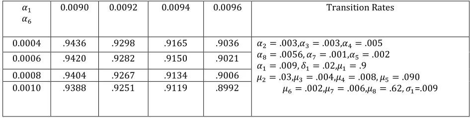
Table 2 Effect of transition ratesF_Dand =_Xon availability of the system

Table 3Effect of transition rates=_Dand =_Von availability of the system

Table 4Effect of PM rate C_D) of the sub system grinding (G) machine on availability

Table 5Effect of PM rate \_X) of the sub system grinding (G) machine on availability

FD

=X

0.0090 0.0092 0.0094 0.0096 Transition Rates

0.056 .9436 .9298 .9165 .9036 =_S= .003,=_$= .003,=_T= .005

=V= .0004,=W= .001,=U= .002

=D= .009, CD= .02,\D= .9

\S= .03,\_$= .004,\_T= .008, \_U= .090

\V= .002,\_W= .006,\_X= .62

0.066 .8710 .8592 .8477 .8367

0.076 .8099 .7995 .7894 .7797

0.086 .7616 .7523 .7433 .7347

=D

=V

0.0090 0.0092 0.0094 0.0096 Transition Rates

0.0004 .9436 .9298 .9165 .9036 =_S= .003,=_$= .003,=_T= .005

=X= .0056, =W= .001,=_U= .002

=D= .009, CD= .02,\_D= .9

\S= .03,\_$= .004,\_T= .008, \_U= .090

\V= .002,\W= .006,\X= .62, FD=.009

0.0006 .9420 .9282 .9150 .9021

0.0008 .9404 .9267 .9134 .9006

0.0010 .9388 .9251 .9119 .8992

CD 0.02 0.04 0.06 0.08

NŠ .9436 ..9440 .9501 .9578

\X 0.60 0.62 0.64 0.66

190

From the tables 1 to 5 we observe that the transition rates of the subsystem D and H affect the availability of the system to run at full capacity. One can see that the result in the table 2 to 5 the failure rate of the subsystem D an H lowers the availability to considerable amount whereas failure rate of the sub system G affect the

availability highly.Therefore, the Grinding

subsystem is the most critical as far as maintenance is concerned and should be taken on topmost priority.

REFERENCES

[1] Krivtosv,V.V. Recent advances in theory and applications of stochastic point process model in reliability engineering, Reliab.Eng.Syst.Safe.92 (2007) 549-551.

[2] Dayer ,D. Unification of reliability/availability models for markov systems IEEE Transaction on reliability 38(1985).

[3] Kumar, D. Availability of the feeding system in the sugar industry Micro electron reliability 28(6) 1988.

[4] Islamov,R.T. Using markov reliability modeling for multiple repairablesystems. Reliability engineering and system safety.1994 113-118. [5] Tsai,Y.,Wang,K..andTsai,L., A study of

availability centered preventive for multi

component system.Reliability engineering and system safety.84(2004) 261-270.

[6] Sharma,R.K. and Kumar,S. Performance modeling in critical engineering system using RAM analysis. Reliability engineering and system safety.93(2008)891-897.

[7] Guo,H., Watson,S.,Taver,P. and Xiang,J. Reliability analysis of wind turbines with incomplete failure data collected from the date of intial installation.Reliability engineering and system safety.94(2009) 1057-1063.

[8] Ke,J.C.and Chu,Y.k. Comparetive analysis of availability for a redundant repairable system.AMC188(2007) 332-338.

[9] Wang,K.H.,Dong,WL.,andKeJ.B.Comparison of reliability and the availability between four systems with warm stand by components and stand by switching failures.AMC 183(2006) 1310-1322.

[10] Uemura,T. and Dohi,T. Availability analysis of an intrusion tolerant distributed server system with preemitivemaintenance,IEEE Transication on reliability.59(1) 2010.

191

µ_X )

µ_D )

µ_D ) µ )

µ )

µ_D )

µ_D ) µ )

µ_W )

µ_W )

µ_W )

µ_X )

µ_X )

µ_X ) FD

CD )

CD ) CD )

=D )

=D )

= )

= )

=X ) =X

=X )

=X )

=D )

=W )

=W )

CD )

‹ $% Œ Œ

• Ž Œ _*O

• Œ Œ _*O 0

3− • 11…15 O $% Œ Œ • Ž Œ _*O

3…7

Ž $% Œ Œ

• Œ Œ _*Ž

24

‹ $% Œ Œ

• Œ Œ _*O

• Œ Œ _*O 0

3− • 9 O $% Ž Œ • Œ Œ _*O

2 ‹

$% Ž Œ

• Œ Œ _*O

• Œ Œ _*O 0

3− • 10 O $% Œ Œ • Œ Œ _*ŽO

• Œ Œ _*O 0

3− 8 O $% Ž Œ • Œ Œ _*Ž

25

Ž $% Œ Œ

• Ž Œ _*O

19…23

Ž $% Œ Œ

• Œ Œ _*O

17

Ž $% Ž Œ

• Œ Œ _*O

18 O

$% Œ Œ

• Œ Œ _*O

1

‹ $% Œ Œ

• Œ Œ _*Ž

• Œ Œ _*O 0

3− •