Splitting compounds with ngrams

Splitting compounds with ngrams

Naomi Tachikawa Shapiro Department of Linguistics

Stanford University Stanford, CA 94305, USA [email protected]

Abstract

Compound words with unmarked word boundaries are problematic for many tasks in NLP and computational linguistics, including information extraction, machine translation, and syllabifica-tion. This paper introduces a simple, proof-of-concept language modeling approach to automatic compound segmentation, demonstrated with Finnish. The approach utilizes an off-the-shelf mor-phological analyzer to split training words into their constituent morphemes. A language model is subsequently trained on ngrams composed of morphemes, morpheme boundaries, and word boundaries. Finally, linguistic constraints are used to weed out phonotactically ill-formed seg-mentations, thereby allowing the language model to select the best grammatical segmentation. This approach achieves an accuracy of∼97%.

1 Introduction

Compound segmentation—the automatic splitting of compounds into their constituent words—is essen-tial to many language processing tasks, including machine translation, information extraction, semantic parsing, spell checking, and syllabification. To that end, we propose a simple, supervised approach to compound segmentation that integrates existing morphological analysis software with language model-ing and optional lmodel-inguistic constraints.

Specifically, the proposed segmenter seeks to identify word boundaries inclosed compounds, com-pounds in which word boundaries go undelimited by spaces, hyphens, or other markers (e.g.,bookworm). These are distinct fromopen compounds, where word boundaries are clearly indicated (e.g.,rain gutter) and thus less of an issue for applications that require their whereabouts. (Note that all compounds are consideredcomplex, while words that are not compounds are consideredsimplex—e.g.,book,rain).

In contrast to previous approaches, which have primarily sought to identify the dictionary forms of compound constituents, this approach aims to identify the exact location of word boundaries in com-pounds. This sort of identification is highly relevant to the domain of computational phonology.

For instance, the location of word boundaries is crucial for syllabification. Closed compounds pose a problem for automatic syllabification because word boundaries form a proper subset of syllable bound-aries; a syllable break will always fall on a word boundary (or, so common phonological theory tells us). Without insight into the location of these boundaries, a rule-based syllabifier might fail to recognize compound-internal word boundaries. For example, ifbookwormis mistaken for a simplex word, English phonotactics would syllabify it as *boo.kworm. Instead, we expect the syllabificationbook.worm, where the syllable break falls on the unmarked word boundary betweenbookandworm.

Hence, we have developed an approach to compound segmentation that specifically identifies word boundaries in compounds, versus lemmatized constituents. In Section 2, we describe previous ap-proaches to compound segmentation in the areas of machine translation and information extraction. We then give a broad sketch of our approach in Section 3, introducing morpheme-based language modeling. Finally, in Section 4, we describe and evaluate an implementation of our approach on Finnish data. This

This work is licensed under a Creative Commons Attribution 4.0 International License. License details: http:// creativecommons.org/licenses/by/4.0/.

implementation uses the morphological analyzer Morfessor 2.0 (Virpioja et al., 2013) and a trigram lan-guage model with Stupid Backoff smoothing (Brants et al., 2007). We also compare our approach to the popular frequency-based method by Koehn and Knight (2003).

2 Related work

Research in compound segmentation has varied in its motivations. While some has focused on improving information retrieval (e.g., Alfonseca et al., 2008) and spell checking (e.g., Huyssteen and Zaanen, 2004) systems, the majority of this work has been tailored to machine translation (e.g., Brown, 2002; Koehn and Knight, 2003; Macherey et al., 2011).

Motivated by a need for translatable constituents, many of these approaches involve multiple lexica and corpora. For instance, Brown (2002) utilizes parallel corpora and a translation lexicon to establish cognates between source and target languages. This allows decompounding into cognate constituents. Brown also proposes an extension to this approach that does not rely on cognate relationships.

Perhaps best known is Koehn and Knight’s (2003) benchmark work on compound segmentation. Though the paper proposes several splitting methods, it is most cited for its frequency-driven approach, which scores candidate segmentations according to the geometric means of their constituents’ corpus frequencies:

ˆ

c= arg max

c∈C (

Y

p∈C

count(p))1n (1)

Above,cˆis the highest-scoring candidate in candidate setC, where each candidatecis composed ofn number of constituent partsp. Candidate sets include all splits into known words, according to a training corpus. Splitting options are further confined to constituents of a minimum length three, and can assume hand-specified letters either inserted or dropped between constituent words, mirroring morphological operations at word joints. This monolingual approach is considered state-of-the-art and serves as a comparison in subsequent work (e.g., Alfonseca et al., 2008; Clouet and Daille, 2014), as well as in Section 4 of this paper.

Also in the domain of machine translation, Macherey et al. (2011) pitch an unsupervised, language-independent approach to compound segmentation. The approach uses phrase translation tables to learn the morphological operations that facilitate compounding, such as the insertion of linking morphemes. It then references a monolingual corpus to assess candidate segmentations. These elements are brought together in a complex dynamic programming algorithm.

Tackling compound segmentation from an information retrieval perspective, Alfonseca et al. (2008) leverage 900 million web documents to determine whether proposed compound constituents exist in anchor texts pointing to the same document. This approach builds on the semantic relationship between compound constituents: “If two words can create a compound word in a language, we can assume that there is some kind of semantic relationships [sic] between them and therefore we would expect to be able to find them near each other in other situations” (134). Alfonseca et al. combine this mutual information feature with lexical, frequency, and probability-based features in a Support Vector Machine classifier.

Efforts in compound segmentation vary widely in terms of the resources they require to get off the ground: monolingual and bilingual corpora, hand-written linguistic rules, web documents, and POS and frequency information. In addition, they have focused largely on the identification of lemmatized constituent words, and not on the identification of compound-medial word boundaries.

3 Compound splitting method

The method of compound segmentation introduced here begins with annotated training data, a set of word forms, both simplex and complex, hand-annotated with any unseen word boundaries. For instance, an annotator would likely mark up the Finnish closed compoundSuomenmaassa‘in the Finnish country’ asSuomen=maassa(suomen‘Finland-NOM’,maassa-INE‘country’). Affix boundaries are not annotated unless they also constitute word boundaries.

An off-the-shelf morphological analyzer is trained on the annotated data and used to segment words into their constituent morphemes (e.g., one might split Suomenmaassainto the morphemes suome, n, maa,ssa). This morphological analyzer is then used to generate candidate compound segmentations and to train a language model.

3.1 Candidate generation

For every morpheme m asserted by the morphological analyzer, there are the four possible bigrams below, where#denotes a word boundary andXdenotes a boundary between two morphemes, or¬#.

#m Xm m# mX

Using this decomposition, candidate segmentations are generated for a word by proposing a word boundary along each of its alleged morpheme boundaries. Suppose that the morphological analyzer takes in the inputwi and outputs the morphemes {m1, m2, m3}. The list of candidate segmentations forwiwould then be every possible combination of internal morpheme boundaries, as shown below. (A word assignednmorphemes will have2n−1 _{candidate segmentations.)}

#m1 #m2#m3# (the most segmented) #m1 #m2Xm3#

#m1 Xm2#m3#

#m1 Xm2Xm3# (the least segmented)

To give a real world example, ifSuomenmaassais split into the constituents {suomen,maa,ssa},1 _it

would yield the following four candidate segmentations:

#suomen#maa#ssa# (suomen=maa=ssa) #suomen#maaXssa# (suomen=maassa) #suomenXmaa#ssa# (suomenmaa=ssa) #suomenXmaaXssa# (suomenmaassa)

One benefit of this approach to candidate generation is that it takes advantage of the linguistic insight that a word boundary will only occur where there is also a morpheme boundary. This reduces the size of the candidate set, compared to approaches that generate candidates by proposing a word boundary in between each letter of a word (e.g., Macherey, 2011), or by recursively proposing all two-part segmenta-tions of some minimum length (e.g., Clouet and Daille, 2014).

Yet, a drawback of this approach is that candidate generation is at the mercy of the performance of the morphological analyzer. If the analyzer fails to identify a morpheme boundary between two morphemes, that boundary will not be considered as a potential word boundary site during compound segmentation.

3.2 Language modeling with morphemes

The intuition behind this segmenter is that the left and right edges of a morpheme each have a certain likelihood of appearing with a word boundary: For some morpheme mi, the bigram ‘#mi’ might be more likely than the bigram ‘Xmi’ (or vice versa), and likewise for ‘mi#’ and ‘miX’.

Consider the English simplex word lighting, composed of the root light and affix -ing (‘#lightXing#’). English speakers know the bigram ‘Xing’ to be extremely common, or, at least, far more common than its counterpart ‘#ing’. This intuition can be captured with language modeling.

Language models are used to assign probabilities to sequences of natural language tokens, typically words and punctuation. A language model sets out to determine the conditional probability of some tokenwi given its historyh(i.e., all of the tokens that precedewi in a training corpus). We approximate the posterior P(w|h)using the Markov assumption thatwi’s history can be estimated through the few tokens that precedewi:

P(wi|h)≈P(wi|wi_i−−_n+11 ) (2) Above,w_ijis a string of tokenswi, ..., wj andnis the order of ngram (i.e.,n= 2for bigrams,n= 3for trigrams, etc.). We can calculateP(wi|wii−−1n+1)by dividing the frequency ofwii−n+1 by the frequency ofwi−1

i−n+1in a training corpus. This gives us amaximum likelihood estimate(MLE) ofP(wi|h):

P(wi|w_ii−₋1_n+1) = count(w i i−n+1) count(wi−1

i−n+1)

(3)

The probability of some sequence of tokenswL

1 is then estimated by taking the product of the MLE for each ngram that appears in the sequence:

P(wL 1) =

L

Y

i=1

count(wi i−n+1) count(wi−1

i−n+1)

(4)

Just as language modeling is used to estimate the likelihood of a sentence, it can be used to predict the likelihood of a proposed compound. Instead of training ngram probabilities on sentences (i.e., sequences of words), we can train them on words, wherein each word is a sequence ofmorphemesandmorpheme boundaries.

Thus, to continue with the English examplelighting, the bigram-MLE of the candidate segmentation *light=ingwould be calculated as follows:

P(#light#ing#) =P(light|#) × P(#|light) × P(ing|#) × (#|ing) (5) Since the bigram ‘Xing’ is far more frequent than ‘#ing’,P(#lightXing#)will receive a higher MLE thanP(#light#ing#). Simply put,P(lighting)> P(light=ing).

As the core component of this segmenter is a language model trained with morphemes, we consider this a morpheme-driven approach to compound segmentation. This is in contrast to word-driven ap-proaches, such as the approaches outlined in the previous section. Word-driven approaches can struggle with accounting for compounds composed of constituent words that were unseen in their training lexicon (see Owczarzak et al., 2014, which addresses this issue). Our segmenter faces this same challenge, but attempts to overcome it by exploiting how, for any set of words, there is generally more information about the distribution of morphemes in the language than the distribution of its words.

3.3 Phonotactic constraints

Using morpheme-based language modeling alone, this approach is vulnerable to predications that are phonotactically ungrammatical, in that it can assert impossible word-internal sequences of sounds. For example, analyzingbookwormas *bookw=ormproduces the unpronounceable constituent *bookw.

To compensate for these ungrammaticalities, linguistic constraints can be posited to prune unsound candidates from the candidate sets. Imagine that we imposed the constraint that all constituent words have at least one vowel. This would discard the candidate compound *boobwo=rm because its con-stituent *rmviolates the constraint.

With a whittled-down candidate set, the segmenter selects the remaining candidate with the highest language model score.

4 Experiment

Data set Total Simplex _Total Complex_{Open Closed} training set 18,079 14,489 3,590 312 3,278

test set 2,001 1,606 395 41 354

Table 1: Training-test set split.

4.1 The data

Aamulehti-1999 contains 16,608,843 words across 61,529 news articles. We extracted a subset com-posed of 20,080 unique word types, including any word that appears one hundred or more times in the corpus.

A single annotator hand-annotated unmarked word boundaries in this subset. The annotator identified 3,632 closed compounds among the 20,080 word types, giving the data the distribution in Table 1. This gold standard underwent a 90-10 train-test split: We used 90% of the annotated data to train both a morphological analyzer and morpheme-based language model. We then evaluated the segmenter on the held-out 10%.

4.2 The segmenter Morphological analyzer

We used a baseline Morfessor 2.0 model (Virpioja et al., 2013) to segment words into mor-phemes. The Morfessor model was trained on raw text consisting of space-delimited data, in which all marked and unmarked word boundaries were indicated with spaces. (E.g., ‘...runoja

raaka-aineen suomen=maassa...’ would have been represented as ‘...runoja raaka

aineen suomen maassa...’.) As needed for candidate generation and the language model, the

model’s viterbi_segment method was used to segment words along their predicted morpheme boundaries.

Language model

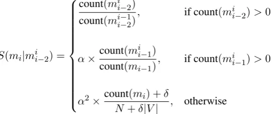
To avoid zero-probabilities (i.e., whereP(sequence) = 0), we used a simple trigram language model with Stupid Backoff smoothing (Brants et al., 2007). The model ultimately backed off to a Laplace-smoothed unigram count, assigning a scoreSto a morpheme/boundarymiaccordingly:2

S(mi|mii−2) =

                        

count(mi i−2)

count(mi_i−₋1₂), if count(mii−2)>0

α×count_count(₍m_mii−1)

i−1), if count(m i

i−1)>0

α2_×count(mi) +δ

N+δ|V| , otherwise

(6)

Above,N is the total number of unigrams seen during training,V is the vocabulary size (i.e., the number of unique morphemes and boundaries), and the Laplace discountδis 1.0. As in Brants et al. (2007), the Stupid Backoff discounting parameterαis 0.4 — it was not tuned to the corpus.

The language model score (SLM) for a candidateciis the product of the score for each morpheme and boundary that appeared inci; this sequence is defined asmL

1:

SLM(ci) =SLM(mL1) = L

Y

i=1

S(mi|mii−2) (7)

To predict the best segmentation ˆcfor a word given its candidate set C, the segmenter selected the candidate with the highest language model score:

ˆ

c= arg max

c∈C SLM(c) (8)

Phonotactic constraints

We formulated four phonotactic constraints that are, in effect, unviolable in Finnish:

• Minimal Word(MINWRD): A candidate incurs a MINWRDviolation for each constituent word that contains fewer than two vowels. (Cf. Suomi et al., 2008). E.g., *a=asian∼aasian, *jun=tunen∼

juntunen, *kä=väisi∼käväisi, *n=uotio∼nuotio, *mat=ala=vaahtoisen∼matala=vaahtoisen, and *ta=lutus=nuorasta∼talutus=nuorasta.

• Sonority Sequencing(SONSEQ): A candidate incurs a SONSEQviolation for each constituent word that begins in a consonant cluster not in /pl, pr, tr, kl, kr, sp, st, sk, spr, str/ or that ends in any consonant cluster. (Cf. Sulkala and Karjalainen, 1992; Suomi et al., 2008). E.g., *luonn=ehti∼

luonnehti, *ehtoisa=mpaa∼ehtoisampaa, and *jukola=ntupien∼jukolan=tupien.

• Vowel Harmony(V-HARMONY): A candidate incurs a V-HARMONYviolation for each constituent word that contains both front vowels /ä, ö, y/ and back vowels /a, o, u/. (Cf. Sulkala and Kar-jalainen, 1992; Suomi et al., 2008; Ringen and Heinamaki, 1999; Karlsson, 2015). E.g., *kesäillan

∼kesä=illan, *taaksepäin∼taakse=päin, and *muutostöitä∼muutos=töitä.

• Word-Final Consonants (WRDFINAL): A candidate incurs a WRDFINAL violation for each con-stituent word that ends in a consonant that is not /t,s,n,l,r/. (Cf. Sulkala and Karjalainen, 1992; Suomi et al., 2008). E.g., *pitem=pään∼pitempään, *sulok=kuutta∼sulokkuutta, and *hyp=pää

∼hyp=pää.

Since these constraints are largely unviolable in Finnish, we designed the segmenter to discard candi-dates that violate the constraints. Given a set of candicandi-dates for an input, for each phonotactic constraint, the segmenter discarded any candidates that violated the constraint, unless it was the case that every candidate violated the constraint. If every candidate violated it, the number of shared violations was subtracted from the number of violations incurred by each candidate. Any candidates that still violated the constraint were then discarded. This is the notion of wiping out shared violations found in Optimality Theory (Prince and Smolensky, 1993/2004).

After using the constraints to pare down the candidate set, the segmenter selected the remaining can-didate with the highest language model score. If no cancan-didates remained, it defaulted to the simplex candidate;3_{this meant that all of the candidates violatedsomephonotactic constraint, but not the same}

constraint equally.

4.3 Evaluation

We evaluated our approach by comparing the segmentations produced by the segmenter to the held-out gold standard. This was done by tallying true and false positives and negatives according to the definitions below. These metrics mirror those used by Koehn and Knight (2003), Alfonseca et al. (2008), Aussems et al. (2013), and Clouet and Daille (2014).

• True positives(TP): Closed compounds that are correctly segmented.

• False positives(FP): Simplex words that are mistakenly segmented.

• True negatives(TN): Simplex words or open compounds that are appropriately left unsegmented.

• False negatives(FN): Closed compounds that the segmenter fails to segment altogether.

• Bad segmentations(Bad): Closed compounds that the segmenter segments, but improperly so.

Using these classifications, precision, recall, and accuracy were calculated, with both precision and recall penalized for bad segmentations:

• Precision= _{T P +F P}T P_+Bad

• Recall= _{T P +F N}T P_+Bad

• Accuracy= _{T P +T N}T P_{+F P}+T N_{+F N+Bad}

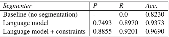
As a probabilistic morphological analyzer, Morfessor predicts slightly different segmentations for the same set of data each time a model is trained. These segmentations consequently impact the ngrams stored in the language model, as well as the constraint interactions further down the pipeline. Due to this variation, we trained a Morfessor model and subsequent language model 50 times on the training set. This was done to ascertain the average performance of each segmenter given the training set and variation from Morfessor. Table 2 portrays the mean precision, recall, and accuracy for using language modeling alone and language modeling with constraints to segment compounds.

Segmenter P R Acc.

Baseline (no segmentation) - 0.0 0.8230 Language model 0.7493 0.8970 0.9373 Language model + constraints 0.8855 0.9201 0.9690

Table 2: Mean performance from training the Morfessor and language models for 50 iterations.

On average, language modeling alone achieved an accuracy of∼94%. In contrast, a language model coupled with linguistic constraints achieved a much higher accuracy, hovering around 97%. Both meth-ods substantially surpassed a baseline of leaving all inputs unsegmented.

Error analysis

To examine specific errors from a representative iteration, we found the iteration that produced accuracies most similar to the mean accuracies depicted in Table 2. The results from this average iteration are shown in Table 3.

Segmenter TP TN FP FN Bad P R Acc.

Baseline (no segmentation) 0 1,647 0 354 0 - 0.0 0.8230 Language model 322 1,553 92 16 18 0.7454 0.9045 0.9370 Language model + constraints 328 1,611 36 18 8 0.8817 0.9266 0.9690

Table 3: Performance from the average iteration.

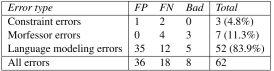
The 62 errors made by the constraint-based (i.e., “language model + constraints”) segmenter fell under one of three types: constraint errors, Morfessor errors, and language modeling errors. The distribution of these errors is summarized in Table 4.

Error type FP FN Bad Total Constraint errors 1 2 0 3 (4.8%) Morfessor errors 0 4 3 7 (11.3%) Language modeling errors 35 12 5 52 (83.9%)

All errors 36 18 8 62

Table 4: Distribution of errors from the “language model + constraints” segmenter.

The correct segmentationmäki=cupwas ruled out due to the loanwordcupviolating MINWRD. And,

brutto=kansan=tuotewas eliminated because the /br/ onset of the Swedish stembrutto‘gross’ violated SONSEQ. In these two cases, all of the candidates violated some constraint and the segmenter conse-quently defaulted to the simplex candidate. Had the correct segmentation not violated a phonotactic constraint, it would have been uniquely identified as the winner.

In the third case, the simplex candidateyksinomaanviolated V-HARMONY, as it contains the front vowel /y/ and back vowels /o, a/.4 _{This led *yksin=omaan to be selected, as it violated none of the}

phonotactic constraints.

The presence of constraint errors cautions us that a segmentation approach that uses phonotactic con-straints is sensitive to loanwords. However, it was only with loanwords where each candidate violated a constraint. This, to some extent, offers loanword detection that falls naturally out of the architecture of the segmenter. This might render it possible to make special considerations for core-periphery structure in the future.

Morfessor errors. The most serious error this segmenter faced was one that stemmed from the mor-phological analyzer. If the mormor-phological analyzer failed to segment a word into its correct constituent morphemes and, in doing so, did not insert a morpheme boundary that also constituted a true word bound-ary, that word’s candidate set did not include the correct segmentation. 11.3% (7/62) of the errors made were Morfessor errors. For example, the segmenter was unable to predict the compoundoheis=krääsän ‘extraneous junk’, since Morfessor split the inputoheiskrääsäninto the constituents {o,hei,sk,rä,ä,sä, n}. Here, the constituentsksubsumes the compound break.

The non-trivial frequency of these errors emphasizes the importance of having a well-trained morpho-logical analyzer.5 _{One way to possibly minimize these errors would be to train the analyzer on words}

annotated for morpheme boundaries instead of word boundaries. (However, morpheme annotation would require more specialized knowledge than compound annotation.) As always, training the morphological analyzer on more data would also likely lead to some improvement.

Language modeling errors. By far the most rampant errors were language modeling errors, totaling 83.9% of the errors (52/62). Language modeling errors arose when, given a refined set of grammatical candidates, the language model favored the incorrect segmentation. Their prevalence is telling about the compound segmentation problem: It highlights the difference between predicting possiblenonword compounds and predictingactualcompounds. It also indicates that the language model is the paramount site for improvement with this approach.

Comparison to frequency-based approaches

We also implemented two versions of Koehn and Knight’s (2003) frequency-based segmenter. Both im-plementations scored candidates solely according to the geometric means of their constituents’ frequen-cies, as in (1). Frequency information and part-of-speech (POS) tags were provided by Aamulehti-1999.

4_{Althoughyksinomaanis left simplex in the gold standard,yksin=omaanis quite arguably the correct segmentation.}

Yksi-nomaanis composed of the stemsyksin‘alone’ andoma-an‘own-ILL’. While the word is semantically noncompositional, evidence from syllabification suggests that it is a compound. Wereyksinomaantruly simplex, its syllabification would be *yk.si.no.maan. However, it syllabifies as if it were a compound, with a syllable boundary falling in between the two stems: yk.sin.o.maan.

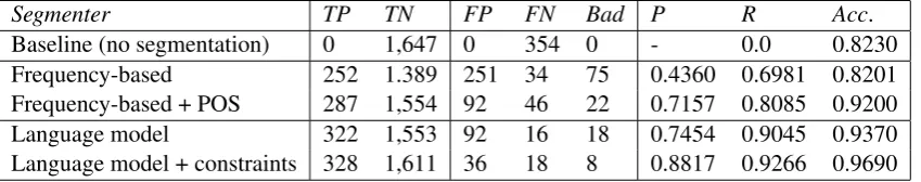
Segmenter TP TN FP FN Bad P R Acc. Baseline (no segmentation) 0 1,647 0 354 0 - 0.0 0.8230 Frequency-based 252 1.389 251 34 75 0.4360 0.6981 0.8201 Frequency-based + POS 287 1,554 92 46 22 0.7157 0.8085 0.9200 Language model 322 1,553 92 16 18 0.7454 0.9045 0.9370 Language model + constraints 328 1,611 36 18 8 0.8817 0.9266 0.9690

Table 5: Performance of the frequency-based and language model segmenters.

The two implementations differed with respect to their candidate sets. The first implementation al-lowed splits into anywords found in the corpus; the second implementation employed POS-filtering, only permitting splits intocontent words (but not proper nouns). Candidate sets for both implementa-tions were restricted to constituents of at least three characters in length.

Table 5 displays the results from evaluating the frequency-based segmenters on the test set; the lan-guage modeling results from the average iteration are repeated for easy comparison. As the table shows, the pure frequency-based approached received 43.60% on precision and 69.81% on recall, culminating in an accuracy comparable to the baseline’s accuracy (∼82%). Both the baseline and frequency-based segmenters were surpassed by the POS-filtered approach, which achieved an accuracy of 92.00%. The language modeling approach achieved a slightly higher accuracy of 93.70%. And, overall, the constraint-based approach achieved the highest precision (88.17%), recall (92.66%), and accuracy (96.95%).

Most notably, the language modeling segmenters earned far fewer false negatives (i.e., higher re-call) than the frequency-based segmenters. This returns us to the issue mentioned in Section 3.2. As word-driven segmenters, the frequency-based approaches struggled with capturing compounds whose constituents did not appear on their own in the corpus. Out of the 46 false negatives produced by the POS-filtered segmenter, 32 occurred because, in each case, one or more of the correct segmentation’s constituents did not appear in Aamulehti-1999 (or did not appear as a content word), precluding it from the candidate set.

On the other hand, as morpheme-driven approaches, the language modeling segmenters largely avoided these errors. (They produced only 3 of the aforementioned 32 errors.) For instance, the frequency-based approaches failed to segment the compoundyli=määräistä‘extra’ (i.e.,yli=määrä-is-tä ‘over=amount-Adj.-PAR’), since the corpus did not containmääräistäas a standalone word. In contrast, the language modeling approaches were able to insert a word boundary in between yliandmääräistä, since the bigram ‘yli#’ surfaced 58 times in the training set, and ‘yliX’ only 17 times.

5 Conclusion

We have proposed a language modeling and constraint-based approach to compound segmentation. This approach was demonstrated with Finnish, a highly agglutinative language. We showed that, by using a morphological analyzer to split words annotated for compound-medial word boundaries into constituent morphemes, we can train a language model that scores different configurations of morphemes, morpheme boundaries, and word boundaries.

Our implementation of this approach used the off-the-shelf morphological analyzer Morfessor 2.0 (Virpioja et al., 2013) and a simple trigram language model with Stupid Backoff smoothing (Brants et al., 2007). This achieved a segmentation accuracy of ∼94%. Then, by layering linguistic constraints on top of the language model, we rooted out phonotactically ill-formed segmentations, allowing the language model to select only grammatical segmentations. This boosted the segmentation accuracy to

∼97%.

Lastly, while this approach was specifically designed to identify word boundary sites in the realm of computational phonology, perhaps it can be adapted for machine translation and information retrieval. For instance, a LEMMA constraint could be added: A candidate segmentation could incur a LEMMA violation for each constituent whose lemmatized form cannot be found in a dictionary or translation lexicon.

Acknowledgements

I am grateful to Arto Anttila for his mentorship throughout this project and to Christopher Manning and the anonymous reviewers for their constructive feedback. In addition, many thanks to Kati Kiiskinen for providing swift and thoughtful annotations of Finnish compounds.

References

Aamulehti. 1999. An electronic Finnish newspaper containing 16,608,843 words. Gatherers: Research Institute for Languages of Finland, the Department of General Linguistics at the University of Helsinki, and the Finnish IT Center for Sciences.

Enrique Alfonseca, Slaven Bilac, and Stefan Paries. 2008. German decompounding in a difficult corpus. In Lec-ture Notes in Computer Science: Proceedings of the 9th International Conference on Intelligent Text Processing and Computational Linguistics, volume 4149, pages 128–139.

Suzanne Aussems, Bas Goris, Vincent Lichtenberg, Nanne van Noord, Rick Smetsers, and Menno van Zaanen. 2013. Unsupervised identification of compounds. InProceedings of the 22nd Annual Belgian-Dutch Confer-ence on Machine Learning, pages 18–25, Nijmegen, Netherlands.

Thorsten Brants, Ashok C. Popat, Peng Xu, Franz J. Och, and Jeffrey Dean. 2007. Large language models in machine translation. InProceedings of the 2007 Joint Conference on Empirical Methods in Natural Language Processing and Computational Natural Language Learning, pages 858—-867, Prague, Czech Republic.

Ralf D. Brown. 2002. Corpus-driven splitting of compound words. In Proceedings of the 9th International Conference on Theoretical and Methodological Issues in Machine Translation, pages 12–21, Keihanna, Japan.

Elizaveta Clouet and Béatrice Daille. 2014. Splitting of compound terms in non-prototypical compounding lan-guages. InProceedings of the First Workshop on Computational Approaches to Compound Analysis, pages 11–19, Dublin, Ireland.

Gerhard B. Van Huyssteen and Menno M. Van Zaanen. 2004. Learning compound boundaries for Afrikaans spell checking. InProceedings of First Workshop on International Proofing Tools and Language Technologies, pages 101–108, Patras, Greece.

Fred Karlsson. 2015. Finnish: An essential grammar. Routledge, London, United Kingdom, 3 edition.

Philipp Koehn and Kevin Knight. 2003. Empirical methods for compound splitting. InProceedings of the 10th conference on European chapter of the Association for Computational Linguistics, pages 187–193, Budapest, Hungary.

Mikko Kurimo, Sami Virpioja, and Ville T. Turunen. 2010. Overview and results of Morpho Challenge 2010. In Proceedings of the Morpho Challenge 2010 Workshop, pages 7–24, Espoo, Finland. Aalto University School of Science and Technology, Department of Information and Computer Science. Technical Report TKK-ICS-R37.

Klaus Macherey, Andrew M. Dai, David Talbot, Ashok C. Popat, and Franz Och. 2011. Language-independent compound splitting with morphological operations. InProceedings of the 49th Annual Meeting of the Associa-tion for ComputaAssocia-tional Linguistics, pages 1395–1404, Portland, Oregon.

Karolina Owczarzak, Ferdinand de Haan, George Krupka, and Don Hindle. 2014. Wordsyoudontknow: Eval-uation of lexicon-based decompounding with unknown handling. InProceedings of the First Workshop on Computational Approaches to Compound Analysis, pages 63–71, Dublin, Ireland.

Catherine O. Ringen and Orvokki Heinämäki. 1999. Variation in Finnish vowel harmony: An OT account. Natural Language & Linguistic Theory, 17(2):303–337.

Helena Sulkala and Merja Karjalainen. 1992.Finnish. Routledge, London, United Kingdom.

Kari Suomi, Juhani Toivanen, and Riikka Ylitalo. 2008. Finnish sound structure: Phonetics, phonology, phono-tactics and prosody. Oulu University Press, Oulu, Finland.