Doctor of Philosophy
California Institute of Technology Pasadena, California
2010
c
2010
I would also like to thank Richard Murray for his wise counsel and especially for allowing me the opportunity to serve in the DARPA Urban Challenge, a truly rewarding experience on so many levels. The support and instruction of my thesis committee members, Pietro Perona and Jim Beck, have been invaluable and for that I am truly appreciative.
I am thankful for the network of people in the Thomas building who have made my time at Caltech enjoyable, in particular Maria Koeper, Chris Silva, and Carolina Oseguera for the wonderful work they do and without whose eorts my defense of this thesis would not have been possible to schedule. A special thanks to Alejandro Delgado for helping me to maintain my oce and the lab. The support of the SOPS community is also much appreciated for the soda, the candy, and the social hours.
The fellowship of the robotics research group is greatly appreciated, for the collaboration and the Ernie's lunches. In particular, I am especially grateful for the friendship and support of my fellow researcher and ocemate Noel DuToit.
I would like to thank my family for their love and their support, which is beyond measure. Thank you for making me the person I am today. A special thanks to Patricia for letting me relive my high school years when graduate school seemed too dicult.
1 Introduction 1
1.1 Motivation . . . 1
1.2 Background and Related Works . . . 2
1.3 Contributions and Thesis Organization . . . 6
2 Background 8 2.1 Bayes' Filter . . . 8
2.1.1 The Kalman Filter . . . 9
2.1.2 The Extended Kalman Filter . . . 11
2.2 SIFT Features . . . 13
2.2.1 Interest Point Detection in Scale-Space . . . 14
2.2.2 Interest Point Selection and Localization . . . 15
2.2.3 Orientation Assignment . . . 15
2.2.4 Keypoint Descriptor . . . 16
2.2.5 Matching . . . 16
2.3 Harris Corner Detectors . . . 17
2.4 Stereo Vision . . . 19
2.4.1 Pinhole Camera Model . . . 20
2.4.2 Two Pinhole Camera Models and Epipolar Constraints . . . 20
2.4.3 Practical Considerations . . . 22
3 Object Detection with 3D Pose Estimation 24 3.1 Object Detection Context and Contribution . . . 24
3.2 Framework . . . 24
3.2.1 Bayes' Filter: Dynamic Prediction . . . 25
3.2.2 Bayes' Filter: Measurement Update . . . 26
4 Sensor Planning for Model Identication 40
4.1 Sensor Planning Context and Contribution . . . 40
4.2 Bayesian Sequential Analysis and Formulation . . . 41
4.2.1 Approach . . . 41
4.2.2 Bayes Filter and Model Probabilities . . . 43
4.2.3 Monte Carlo Sampling . . . 44
4.3 SPPEMI Algorithm . . . 45
4.3.1 Function: calcCurrentEntropy(·) . . . 46
4.3.2 Function: calcPossibleControlActions(·) . . . 46
4.3.3 Function: calcExpectedEntropy(·) . . . 47
4.4 Case Study . . . 48
4.4.1 Motion Model . . . 49
4.4.2 Measurement Model . . . 49
4.4.3 Applying the Algorithm . . . 50
4.4.4 Simulated Results . . . 52
4.4.4.1 m=4, n=6 . . . 53
4.4.4.2 m=6, n=8 . . . 54
4.4.4.3 m=8, n=10 . . . 56
4.5 Practical Considerations . . . 57
5 Implementation of SPPEMI 58 5.1 Experiment 1: Constrained Mobile Agent and Object . . . 58
5.1.1 Motion Model . . . 59
5.1.2 Measurement Model . . . 62
5.1.3 Applying the Algorithm . . . 63
5.1.4 Results . . . 67
5.2 Experiment 2: Mobile Agent with Mobile Object . . . 70
6.2.2 Global Search Method . . . 82
6.2.3 Local Search Method with 6D Pose Estimation . . . 84
6.2.4 Robot Navigation and the Costmap . . . 86
6.3 Approach Summary . . . 87
6.4 Experimental Results . . . 88
6.4.1 Robustness to Height Variance . . . 88
6.4.2 Robustness to Obstacles and Re-planning . . . 90
6.4.3 Additional Tests and Search Limits . . . 92
6.4.4 Extensions to Multiroom Search . . . 94
6.5 Conclusions . . . 96
7 Conclusion and Future Work 97 7.1 Discussion and Summary of Work . . . 97
7.2 Conclusions and Future Work . . . 98
A Linearized Measurement Matrix 99
B Motion Model for Unconstrained Motion 101
2.3 Harris corner detection overview . . . 18
2.4 Harris corner detector example . . . 19
2.5 Background: pinhole camera model . . . 20
2.6 Background: epipolar geometry for stereo camera model . . . 21
2.7 Background: 3D depth image generated from stereo reprojection. . . 22
3.1 Object-detection: database feature generation overview . . . 28
3.2 Object-detection SIFT region of interest (ROI) overview . . . 32
3.3 Object-detection algorithm block diagram . . . 33
3.4 Object-detection experimental setup . . . 34
3.5 Object-detection ground truth setup . . . 35
3.6 Object-detection experiment 1: results . . . 36
3.7 Object-detection experiment 2: results . . . 37
3.8 Object-detection visual interface screenshot . . . 38
4.1 Sensor-planning motivation . . . 41
4.2 SPPEMI case study polygon example . . . 48
4.3 SPPEMI case study measurement model . . . 50
4.4 SPPEMI case study simulated results, (m=4, n=6) . . . 53
4.5 SPPEMI case study simulated results, (m=6, n=8) . . . 55
4.6 SPPEMI case study simulated results, (m=8, n=10) . . . 56
4.7 SPPEMI algorithm block diagram . . . 57
5.1 Sensor-planning experiment 1: setup . . . 59
5.2 Sensor-planning experiment 1: frame transformations . . . 60
5.3 Sensor-planning experiment 1: model descriptions . . . 67
5.4 Sensor-planning experiment 1: pose estimation results . . . 68
5.5 Sensor-planning experiment 1: model probability values . . . 69
6.5 Object-search experimental object models . . . 88
6.6 Object-search experimental results (varied height) . . . 89
6.7 Object-search experimental results (obstacle avoidance) . . . 90
6.8 Object-search experimental object models (additional) . . . 91
6.9 Object-search experimental results (additional objects) . . . 91
6.10 Object-search failed search experiment (tin can) . . . 92
6.11 Object-search failed search experiment (penguin cup) . . . 93
6.12 Object-search simulated multiroom search . . . 95
4.3 SPPEMI case study table of models, (m=8, n=10) . . . 56
This thesis develops new methodologies for 3D object detection and tracking in vision with applica-tions to sensor planning and object search. Motivation for this research will be discussed, highlighting the need for the main contributions of this work. Previous works will briey be reviewed and an outline of the thesis contributions made will be given.
1.1 Motivation
A large part of robot autonomy is characterized by perception, the ability of a robot to sense its environment and interpret it in an intelligent way. While humans have been able to solve this problem with only a few types of proprioceptive and exteroceptive sensors, the robotic systems of today typically require a large number of exteroceptive sensors coupled with a signicant source of computing power. Nonetheless, signicant advances in perception have still been made with applications in military defense, assisted driving, and even home living.
One of the rapidly maturing areas of robot perception has been in the eld of computer vision where the primary sensor is a camera and sensory data comes in the form of images grayscale and color. Historically, limitations in computing bandwidth have restricted many algorithms to o-line batch implementation, with real-time processing issues less well explored. Not until recently, the expense of high-quality, precision cameras limited many algorithms to using a single monocular camera sacricing the richness of data available from a second camera (such as in stereovision applications).
With the recent advent of faster computers and cheaper cameras, real-time processing of vision data from multiple cameras has become much more common in robotics research over the past decade. A particular problem enabled by the availability of modern hardware is 3D object-detection with tracking. While past methods have achieved robust object-detection in static images ([18] provides a good review), the following section will discuss the recent advances that have extended existing methods to real-time 6D pose estimation.
1.2 Background and Related Works
The problem of 3D object detection and tracking is not a new one and has seen its fair share of proposed solutions. However, much of the prior work on object detection has focused on o-line computation thereby limiting the real-time tracking aspect. In this context of 3D object recognition, most approaches rst detect and recognize an object, then estimate its 6D pose. Of the developed methods, a majority of them can be classied as either appearance based ([23], [26], [43], [45]) where descriptors (i.e., features) derived from images of the object are utilized, or geometrical based ([7], [28], [36], [50]) where geometric models are constructed for each object and shape-matching techniques (e.g., aspect-graphs) are then used. In either case, a training-phase is rst implemented whereby the object is rst learned from varying viewpoints a process that accounts for detection from any number of possible viewing angles. While a majority of research has shifted towards appearance-based methods due to the success of various approaches in recent years, the related problem of feature-correspondence (i.e., matching features detected in the image with the correct features on the known object) has become equally important ([9]).
mismatches. Their method utilizes a set of calibrated images of the object with the 3D geometric model, and image feature correspondence is achieved via a combination of PCA and a Bayesian classication framework where a 1.53 Hz tracking rate is possible with a monocular camera. Vac-chetti et al. in [54] take an approach similar to [36], yet achieve tracking rates at about 2530 Hz for 320×240 sized images from a monocular camera. In their approach, batch methods are used to
generate a 3D object model from a series of keyframes, and object pose estimation is realized by matching features between the test image and the closest keyframe. Drawbacks of their approach, however, are the requirement that the object be close to a known keyframe to ensure robust object registration and the algorithm's sensitivity to scale and rotation changes which is a direct result of the corner patch features chosen by the authors.
With the introduction of SIFT features in 1999 by David Lowe [29], many previous problems associated with feature mismatches caused by scale or rotational variance have been alleviated, allowing greater accuracy and stability. Panin and Knoll [40] introduce a real-time solution that is invariant to scale and rotation via SIFT. Their approach uses a monocular camera and SIFT features to detect and initialize an object with sustained tracking achieved by switching to a contour-based tracking algorithm. Choi et al. in [5] extend the work of Panin and Knoll by demonstrating real-time 6D pose estimation and tracking for both monocular and stereo cameras. Rather than applying SIFT-base feature matching on each frame, the object pose is only initialized using SIFT (similar to the approach of [40]), and then a Lucas-Kanade (LK) tracker [31] is used. Pose estimation for the monocular case is done using the POSIT algorithm [10], while a closed-form solution involving unit quaternions handles the stereo case. However, their proposed system is susceptible to large delays caused by SIFT reinitialization when tracks are lost due to large object motions.
information on its whereabouts. It investigates solutions to the similar question: how should one move next to improve the probability of object detection and localization?
In previous years, the problem of sensor planning has been considered in the context of various applications: autonomous driving ([52], [41]), object search ([56]), visual mapping ([8],[51]), multiple target detection and tracking ([20], [48], [22]). The application of sensor planning to the problem of model identication has also been investigated to some extent. In computer vision, the problem is often categorized as an active recognition problem ([4], [44]), i.e., determining the appropriate set of actions to execute for a visual agent to gather enough evidence to disambiguate initial object hypotheses. Recently, the application of information theoretic concepts has been investigated as a possible solution in o-line and on-line methods to this problem.
Arbel et al. [1] consider an approach that discretizes the viewing sphere around an unidentied object and populates grid cells with entropy values. Notable in their work is that sensor planning for object recognition is achieved by selection of the most informative view based on the precom-puted entropy maps. Paletta et al. in [39] take a more practical approach and present a Bayesian fusion method that incorporates the temporal context of observations by integrating multiple recog-nition results. Through a Markov Decision process, a planning scheme is selected that minimizes the expected entropy loss. Their proposed real-time algorithm shows interesting results for object classication using Bayesian sequential recognition. However, their work lacks in its ability to track and estimate the 6D continuous pose of model objects.
approach suers when applied to real data images, as opposed to simulated views.
It is clear that the problem of sensor planning for model identication has yet to incorporate simultaneous, on-line 6D pose estimation in any of the above methods. Chapter 4 will present an information theoretic approach to sensor planning that shows via Bayesian analysis that object pose estimation is not only an added feature but a necessary step to the next-best-view calculation. Fur-thermore, the object itself is no longer conned to a stationarity assumption and active recognition in a dynamic setting is explored.
The problem of object-search has been considered as an element of sensor planning research in recent years as well. Ye and Tsotsos in [56] developed one of the rst systematic frameworks for object search that incorporated both sensor planning and object recognition. Their method was developed for a two-wheeled robot equipped with a pan-tilt-zoom camera and a laser eye. Their spherically arranged training data set encodes the probability that a given sensor movement on a sphere surrounding the object will improve detection. Their computationally expensive method can be tedious to implement given its need for the experimental construction of a detection function for all sensing parameters (pan, tilt, zoom, robot orientation) under various lighting conditions, object orientations, and background eects. Furthermore, the object recognition function is limited to a 2D technique using a blob nder based on pixel intensity.
More recently, Saidi et al. ([46], [47]) extend the work of Ye and Tsotsos to a humanoid robot where object recognition is carried out via 3D SIFT features. They present a visual attention framework that relies upon pan-tilt-zoom capabilities to generate 3D data of the sensed environment. They formulate search as the problem of optimizing sensor actions and trajectories with respect to a utility function that incorporates target detection probability, new information gain, and motion cost. A visibility map similar to the sensed sphere of [56] lters uninformative sensing actions. While their approach is a signicant improvement on the work of Ye and Tsotsos, the visibility map calculations are computationally expensive and their utility function lacks a formal Bayesian framework.
addressed, a crude object recognition system is used, and object pose estimation is limited to the process of aligning the current object image with a predened reference image an approach that works only on piecewise planar objects in positions that match the reference image and pose.
Building and improving upon the work of Petersson et al., Ekvall et al. [14] and Lopez et al. [27] decompose the object search problem into global and local search stages. Their coarse global search employed Receptive Field Coocurrence Histograms [13] to identify potential object locations. A mobile robot equipped with laser, sonar, and a pan-tilt-zoom camera then zooms into each hypothesized location to apply a localized object search algorithm (based on SIFT features). An a priori map built via SLAM is used to establish likely locations of known objects. Navigation is restricted to planning over a graph of predetermined free-space nodes. This approach simplies the methods of [56] and [47] and allows for simultaneous search of multiple objects. However, their approach is limited to planar objects whose pose is crudely approximated by a single laser scan point in [14] and later moderately rened in [27] to a distance measure based on comparing the number of occupied pixels in the image against a reference image. Furthermore, much prior information is assumed given or computed o-line (e.g., the SLAM-based map and the set of navigation nodes). The contributions of chapter 6 will improve on the work of [56] by using a 3D object detector and will also simplify the method of [47] by replacing the computationally expensive 3D visibility map and rating function with a global and local search technique that updates the grid-based probability map incorporated from [6].
1.3 Contributions and Thesis Organization
The contributions and organization of this thesis are as follows. Chapter 2 establishes technical background that supports the contributions in later chapters. It presents existing techniques and strategies used in control theory and computer vision.
estima-chase of third-party software as in [54], simulated experimental results as in [40], or distinguishing markers for computer vision toolkits as in [5].
Chapter 4 presents a novel approach to sensor planning that incorporates the 6D pose esti-mation algorithm developed in chapter 3. Using Bayesian analysis, the Sensor-Planning-for-Pose-Estimation-and-Model-Identication (SPPEMI) algorithm is derived. It solves for the optimal action for the next-best-view which optimizes an information gain metric. While the previous works of [1], [11], [12], [25], [38] and others considered static objects in conned workspaces, the derived approach makes no assumptions on the workspace, allowing for mobile objects sensed from mobile platforms. Chapter 5 presents two specic experiments to highlight the applicability of the algorithm in chapter 4 in real-time. The rst experiment considers a mobile object and mobile agent both of which are constrained in their movements to the projected viewing sphere, illustrating the capabilities of the overall SPPEMI algorithm to consider mobile objects. In the second experiment, unconstrained motion of the object and the viewing agent are considered demonstrating the success of the overall method to initialize a potential object, plan a sensor motion for improved sensing, and simultaneously track and estimate an object's pose all while executing the planned sensing action.
Chapter 6 considers another application of the 3D tracking algorithm of chapter 3 to the object-search problem, where a global and local object-search decomposition is used to not only locate the object but accurately estimate its 6D pose as well. A method is presented whereby an autonomous mobile robot searches for a 3D object using an onboard stereo camera sensor mounted on a pan-tilt head and estimates the 6D pose of the object once found. Search eciency is realized by the combination of a coarse-scale global search coupled with a ne-scale local search over a grid-based probability map which is updated using Bayesian recursion methods. A grid-based costmap is also populated from stereo and used to facilitate obstacle avoidance and path-planning. Experimental results obtained from the use of this method on a mobile robot are also presented in this chapter to validate the approach, conrming that the search strategy can be carried out with modest computation.
This chapter reviews fundamental concepts, algorithms, and necessary equations that support the overall work of this thesis. Since this work entails a great deal of 3D position estimation, section 2.1 presents a brief outline of the Bayes' Filter, a recursive tracking lter derived from the principles of Bayes' Law and is a form of Bayesian Sequential Updating. Section 2.2 presents an overview of SIFT (Scale-Invariant-Feature-Transform) features, a vision-based feature set rst developed by David Lowe ([30]) and used in this work (and by other researchers as well) for their strong discriminating capabilities that greatly simplify the data association problem between measurements in images and the state elements to which they measure. Section 2.3 presents an overview of another type of vision-based feature developed by C. Harris and M. Stephens in [17], known as the Harris corner detector.1 Harris corners are computationally aordable (and thus faster), though less robust to scale and rotation variance than SIFT features. Lastly, a major element of this thesis relies on accurate stereo-reprojection of 2D pixels to their corresponding 3D location in Cartesian space. Section 2.4 presents a brief review of epipolar geometry as applied to two optically aligned cameras which enables stereo vision in the most common sense.
2.1 Bayes' Filter
Bayes' Filter is a recursive algorithm derived from Bayes' Law that allows the state of a system to be represented by a probability distribution or a belief. In the eld of robotics, the state of the system is often dened as the position and orientation of the robot, and the Bayes' Filter is a means of incorporating sensory data to update and continuously estimate the pose of the robot.
Let Xk ∈ Rn×1 be a continuous random variable representing the system state at the k-th
timestep, D1:k ∈Rm×1 a continuous random variable representing the direct or indirect
measure-ments of the system from timestep1 up to and including timestep k, and u1:k ∈ Rb×1 the
corre-sponding control inputs to the system.2 Then Bayes Filter is a recursive algorithm which cycles
1Harris corners are also sometimes referred to as Kanade-Tomasi corners, where the latter authors developed an
improved version of the original algorithm by Harris and Stephens, by replacing the original corner measure with the minimum eigenvalue.
measure-2.1.1 The Kalman Filter
As an exercise, one can consider the particular case when the state is governed by linear dynamics and the measurements linearly dependent on the state of the system with only Gaussian noise. In this particular case, two propositions will prove useful in analytically solving the expressions of Bayes Filter. The propositions will be stated here and the proofs can be found in [53].
The rst proposition deals with the integral of the product of two multivariate normal distribu-tions and is useful in solving the dynamic prediction step of the lter:
Proposition 2.1: LetN(x;f(y,u),Σx)be a normal distribution over the continuous random vari-able x with mean f(y,u) and covariance Σx. Let f(y,u) be a linear function in y and u of the
following form:
f(y,u) =Ay+Bu+C.
Similarly, let N(y;µy,Σy) be a normal distribution over the continuous random variable y with meanµy and covarianceΣy. Then the integral over yof the product of both normal distributions is itself a normal distribution, with mean and covariance given by
N(x;µ∗,Σ∗) =
Z
N(x;f(y,u),Σx)·N(y;µy,Σy)dy,
µ∗ = f(µy,u),
Σ∗ = AΣyAT + Σx.
The second proposition provides an analytical solution to the product of two multivariate normal distributions, and is useful in solving the measurement update step:
Proposition 2.2: LetN(y;f(x,u),Σy)be a normal distribution over the continuous random vari-able y with mean f(x,u) and covariance Σy. Let f(x,u) be a linear function in x and u of the
where:
µ∗=µx+K(y−f(µx,u)),
Σ∗= (I−K·C)Σx,
K= ΣxCT(C·Σx·CT + Σy)−1.
With the above propositions dened, now consider the following system dynamic model and mea-surement model:
Xk=A·Xk−1+B·uk−1+wk−1, (2.3)
Dk=C·Xk+vk, (2.4)
where A ∈ Rn×n, B ∈ Rn×b, and C ∈ Rm×n are state independent matrices and wk−1 ∈ Rn×1
andvk−1∈Rm×1 represent Gaussian white process and measurement noise governed by covariance
matricesQ∈ Rn×n andR∈Rm×m, respectively. The Bayes' Filter as dened by equations (2.1)
and (2.2) can be analytically solved using propositions 2.1 and 2.2. Beginning with the dynamic prediction step, the belief of the state of the system is predicted forward as follows:
p(Xk|D1:k−1,u1:k−1) =
Z
N(Xk|A·Xk−1+B·uk−1;Q)·N(Xk−1|µk−1; Σk−1)dXk−1
=N(Xk|µk; Σk),
where the termsµk andΣk are given by:
µk=A·µk−1+B·uk−1, (2.5)
Σk=A·Σk−1·AT +Q. (2.6)
Σk = (I−Kk·C)Σk, (2.8)
Kk = ΣkCT(C·Σk·CT +R)−1. (2.9)
As should be obvious, the Bayes Filter reduces to the well-known Kalman Filter under linear system, Gaussian noise assumptions. Equations(2.5) and (2.6) implement the Kalman prediction step and equations (2.7) and (2.8) implement the Kalman update step with the dynamic Kalman gain given by equation (2.9). Note that the Kalman gain is a matrix that optimally weights the termDk−C·µ−k (often referred to as the innovation or the measurement residual) such as to minimize the covariance of the error between the true state of the system and the best estimate of that state. While the derivation of the Kalman Filter as shown here is brief, references [32] and [55] provide more rigorous derivations.
2.1.2 The Extended Kalman Filter
Now consider the case when the system to be estimated does not have linear dynamics nor are the measurements linearly dependent on the state. Bayes' Filter can still be applied by approximating the system as locally linear.3 Since the system is assumed non-linear, the system dynamic model and measurement model are dierent and generalized to be
Xk =F(Xk−1,uk−1,wk−1), (2.10)
Dk =H(Xk,vk), (2.11)
where the variablesXk,uk−1,wk−1(∼N(0;Q)),and vk(∼N(0;R))are as previously dened for the linear case and F(·) ∈ Rn×1 and H(·) ∈
Rm×1 are non-linear functions that depend on the
state and control variables and process/measurement noise. By applying the linear approximations,
3The particle lter is another method of applying Bayes' Filter to non-linear systems. However, they can be
With the linear approximations as dened above, the Bayes' Filter is then carried out in a manner analogous to the linear case. Beginning with the dynamic prediction step, the belief of the state of the system is predicted forward as follows:
p(Xk|D1:k−1,u1:k−1) =
Z
N(Xk|F(Xk−1,uk−1,0);Q)·N(Xk−1|µk−1; Σk−1)dXk−1
=N(Xk|µk; Σk),
where the termsµk andΣk are given by
µk=F(µk−1,uk−1,0), (2.12)
Σk=Ak−1·Σk−1·ATk−1+Q. (2.13)
The measurement update step of Bayes Filter is then implemented with linear approximations as follows:
p(Xk|D1:k,u1:k−1) =η·N(Dk|H(Xk,0);R)·p(Xk|D1:k−1,u1:k−1)
=η·N(Dk|H(Xk,0);R)·N(Xk|µk; Σk)
=N(Xk|µk; Σk),
where the termsµk andΣk (and the Kalman GainKk) are given by
µk =µk+Kk(Dk−H(µk,0)), (2.14)
Σk = (I−Kk·C)Σk, (2.15)
Kk = ΣkCT(C·Σk·CT +R)−1.
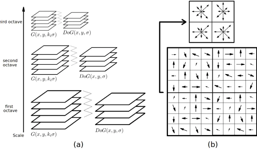
Figure 2.1: (a) Interest point detection is achieved by applying the Dierence of Gaussians (DoG) operator in between adjacent levels of Gaussian blurred images within the same scale. The set of Gaussian blurred images within a scale dene an octave. Each additional octave is then created by downsampling the image and repeating the calculations of determining the DoG images. (b) The feature descriptor is composed of an orientation histogram generated over a 4x4 sample region computed from a 16x16 sample array, though shown in the gure is a 2x2 region from an 8x8 sample array.
prediction step and equations (2.14) and (2.15) correspond to the EKF update step. It is important to note that the EKF is an adhoc approach of approximating non-linear systems as linear. In many cases, the system does not behave locally linear and the EKF should not be applied. Furthermore, the system and measurement noise will not necessarily follow a normal distribution after going through the non-linear transforms of F(·)and H(·)and is fundamentally inaccurate. Nonetheless,
rather good results can be achieved for state estimation of non-linear systems with these linear approximations.
2.2 SIFT Features
3. Orientation assignment: For all stable interest points selected, an orientation based on local image gradient directions and magnitudes is assigned. If multiple viable orientations exist, then new interest points are generated with identical localized positions and scale, yet diering orientation.
4. Keypoint descriptor: To handle invariance to rotation, each interest point is rotated up to
360◦ in 8 steps, relative to the interest point dominant orientation. For each stepped rotation
of the interest point, an orientation histogram is generated over a 4x4 sample region computed from a 16x16 sample array. This yields a 128-element descriptor.
Each of the above steps will now be discussed in further detail to provide a better understanding of how the exact features achieve invariance properties.
2.2.1 Interest Point Detection in Scale-Space
Interest point detection in scale-space is achieved by applying a Dierence of Gaussians (DoG) operator between various scales of the image. This is done by rst considering the original image and creating an octave of Gaussian blurred copies of the original image, with each copy convolved with a Gaussian at a diering variance oset by a multiplicative constantk; that is
D(x, y, σ) = (G(x, y, kσ)−G(x, y, σ))∗I(x, y),
whereG(x, y, kiσ)is given by
G(x, y, kiσ) =
1 2πσ2
i
e−(x2+y2)/(2(kiσ)2).
curvature is checked for each point, to ensure the interest point does not lie simply on an edge. To avoid direct computation of the eigenvalues, Lowe borrows from the approach of Harris and Stephens in [17] and needs only to calculate the trace and determinant of the Hessian matrix and subsequently check the ratio of the two against some threshold,r, i.e.,
H=
Dxx Dxy
Dyx Dyy
,
T r(H)2
Det(H) <
(r+ 1)2
r ,
which in Lowe's implementation, the ratioris set tor= 10. Once the interest points are selected,
the orientation of the interest point is next set.
2.2.3 Orientation Assignment
For each interest point selected with some associated scale, the local orientation of image gradients is then considered. That is, for the interest point (xi, yi), the corresponding Gaussian blurred image closest in scale is selected. A histogram of gradient orientations (organized into 36 bins to span the360◦ of orientation) is then generated for a small neighborhood of pixels surrounding the
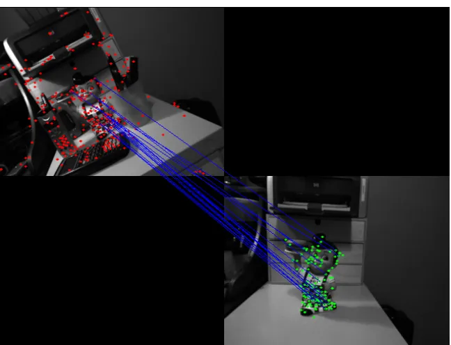
Figure 2.2: The above display shows the quality of feature matching achieved with SIFT features and the Best-Bin-First search algorithm. The object to recognize is displayed in the bottom right image. In the top left image, a cluttered and rotated scene containing the object is presented. Note the large number of matches (shown in blue) that exist despite the distractors, rotation, and partial occlusion.
2.2.4 Keypoint Descriptor
In this nal step, invariance to rotation is achieved via careful construction of the interest point descriptor. This is done by rotating the interest point360◦in 8 rotation steps, relative to the interest
point orientation assigned in the previous step. For each stepped rotation, an orientation histogram is generated over a 4x4 sample region computed from a 16x16 sample array. This yields a 128-element descriptor which improves the probability of accurately establishing feature correspondences across various rotations of the image scene. Figure 2.1(b) illustrates schematically how the orientation histograms might be computed for a given orientation and what the resulting sample region might look like.
2.2.5 Matching
yield many mismatches that are undesirable. By comparing how well a feature matches to its nearest neighbor and its second nearest neighbor allows one to consider how far isolated the nearest neighbor match truly is (i.e., if the ratio of the two matched distances is small enough, then a valid correspondence is likely to have been found and should be kept).
The motivation behind the second simplication is more practical for implementation purposes. The Best-Bin-First search algorithm returns with high probability a feature's nearest neighbor by utilizing an ordered k-d tree. The search order itself requires the use of a heap-based priority queue that yields a speedup of search time by about two orders of magnitude. Figure 2.2 presents an example of the matching results for SIFT features used on a given object. The object to be matched is shown in the bottom right image and the presented scene image is shown in the top left. Note that despite the rotation of the scene image and large number of distractors, robust matching is still achieved.
2.3 Harris Corner Detectors
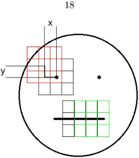
Corner detection is perhaps one of the rst forms of feature extraction from images used in the eld of computer vision. It began with the seminal work of Hans Moravec [34] whose approach to corner detection was to consider for each pixel a patch centered on that pixel and computing a weighted Sum-of-Squared-Dierences (SSD) against a small set of neighboring patches generated by slight
variations of the center pixel inxandy:
SSD=X
u X
v
w(u, v)(I(u, v)−I(u+x, v+y))2,
wherew(u, v)is some nominal weight applied to the calculated Sum-of-Squared Dierence, calculated
as a function of pixel location. Figure 2.3 illustrates the concept behind Moravec's approach. Pixels at corners typically yield large values in all translations of x and y whereas pixels at non-corner
Figure 2.3: Corners are detected by generating a patch at a certain pixel location and calculating a Sum-of-Squared-Dierence (SSD) between that patch and a set of neighboring patches. Pixels
at corners (e.g., the red patch) typically yield large values in all translations of x and y whereas
pixels at non-corner locations (i.e., noise) typically yield low overall values. With regards to edges (e.g., the green patch), the SSD can be prominent in translations ofxandy perpendicular to the
direction of the edge and low for translations ofxandy along the edge.
translations ofxandy perpendicular to the direction of the edge and low for translations ofxand y along the edge until it reaches the ends of the edge when it reaches a maximal SSD value. One
of the major drawbacks of Moravec's approach was that his operator was not isotropic in the sense that if an edge ran a direction not consistent with a translation to a neighboring pixel, then it would fail to be picked up as a corner.
In 1988, Harris and Stephens improved on the approach of Moravec in their seminal paper [17] by making the operator isotropic by performing an analytical expansion about the shift origin:
SSD=X
u X
v
w(u, v)(I(u, v)−I(u+x, v+y))2
≈X
u X
v
w(u, v)(Ix(u, v)·x+Iy(u, v)·y)2, (2.16)
where Ix= ∂I∂xand Iy = ∂I∂y represent the image gradients inxandy at the (u, v)pixel. Note that equation (2.16) is often re-written in the following matrix form:
SSD≈[ x y ]A
x y ,
A=X
u X
v
w(u, v)
Ix IxIy
IxIy Iy
.
With the SSD so formed, Harris and Stephens noted that the existence of corners can be easily
deduced by the eigenvalues of the matrix A, namely that if the eigenvalues(α, β)are both large,
Figure 2.4: The above gure illustrates the application of the Harris corner detector to a given image shown on the left and the resultant detected corners shown in red on the right.
that this calculation holds only for one proposed shift in the center pixel by(x, y). In their proposed
operator, Harris and Stephens took a conservative approach and declared a corner exists only if the response to their operator for all 8 possible neighboring shifts yielded a local maximum.
Lastly, to avoid computationally expensive operations for eigenvalue decomposition, an alter-native metric is used when calculating Harris corners termed the corner response and is dened by
CR=Det(A)−k·trace(A)2.
This metric serves as a feasible alternative to the eigenvalue comparison, with the constantkoften
chosen in the range of0.04−0.15.
One of the benets of the Harris corner feature, when compared to more sophisticated features like SIFT, is its speed. Figure 2.4 illustrates a simple application of the Harris operator to a given image scene, which is a 640×480 image that took 0.04 s to compute roughly 300 corners on a modest
laptop computer with a 1.86 GHz processor.
2.4 Stereo Vision
Figure 2.5: The pinhole camera model commonly used to describe the interworkings of most CMOS/CCD cameras.
2.4.1 Pinhole Camera Model
A common model used for most cameras is the pinhole-camera model, as shown in Fig. 2.5. The model consists of an image plane, some distancef known as the focal length and typically measured
in pixels from the center of projection, denoted byO. Image coordinates are represented in pixels
(x, y) measured relative to the image center (cx,cy). Using similar triangles, a point in 3D Euclidean space (X, Y, Z) can be transformed into image coordinates using the following relation:
x=f ·X
Z , (2.17)
y=f ·Y
Z . (2.18)
Note that going from 3D point locations to 2D image locations is a straightforward process, yet the converse is not possible unless the depthZ of the (x, y) pixel is known, or another equation is
introduced. Alternatively, with a second camera, this slight complication can be remedied.
2.4.2 Two Pinhole Camera Models and Epipolar Constraints
Consider the diagram of Fig. 2.6(a) which shows two pinhole camera models. Let the reference camera in this case be the right camera (an arbitrary choice). Note that in the gure both cameras do not have coplanar image planes. Nonetheless, this serves as a good opportunity to briey discuss epipolar geometry. An epipole is dened as the point of intersection with the image planes of the line joining the optical centers of both cameras (el and er in Fig. 2.6a). When a point P0 ∈ R3
is seen in the reference image, its location in the other image can potentially be anywhere along the line (called the epipolar line) generated by the intersection of the epipolar plane (i.e., the plane formed by the epipoleserandel and the pointP0) and the image plane of the other camera.
Figure 2.6: (a) A schematic explaining the epipolar geometry associated with two pinhole camera models. (b) For two cameras that have coplanar image planes and co-linearx−axes, the epipolar
line associated with a pointP0is reduced to the same horizontal row at which the point was detected
in the reference image.
axes, and colinear x-axes separated by a distance B as shown in Fig. 2.6b. In this particular
case, the epipolar geometry reduces the epipoles of both cameras to lying on the same rows in each image plane. As such, the epipolar lines coincide with horizontal rows of the image and image point correspondences can be reduced to search along rows.
The pixel distance between the image point ofP0in the reference camera (p0,r= (x0,r, y0,r)) and the found correspondent point in the secondary image (p0,l = (x0,l, y0,l)) is dened as the disparity,
d0:
d0=x0,l−x0,r.
Note that xi,l > xi,r always. Knowing the disparity and the separation distance between cameras (baseline)B, the following relation can be used to determine the depth associated withp0,r (using similar triangles):
Z0=
f·B d0
,
and withZ0 known, the distance inxandy can be deduced from equations (2.17) and (2.18):
X0=
x0,r·Z0
f ,
Y0=
y0,r·Z0
f .
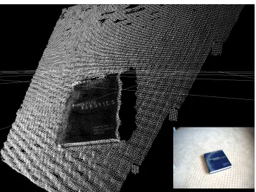
Figure 2.7: Shown is a plot of 3D stereo reprojected data using a stereo camera with a baseline of
0.12m. The reference image is shown in the bottom right.
2.4.3 Practical Considerations
For the two pinhole-camera models described above, the simple case of both cameras having coplanar image planes and parallel optical axes was considered. However, in all real-life situations, cameras in that conguration are never perfectly aligned no matter how well calibrated a stereo-camera pair may be. Furthermore, there are barrel aects associated with all types of lenses that produce distortion around the periphery of the image resulting in non-linear eects which invalidate the horizontal epipolar line assumption. Lastly, the CMOS or CCD chip of the camera is never perfectly aligned with the optical axis. As such, the focal length f is rather dicult to come by, typically resulting
in two components that need to be accounted for: the focal length inx(fx) and the focal length in y (fy).
Oftentimes much of these practical issues can be accounted for by calibrating the cameras and applying transformations to the image in the form of distortion coecients that serve to rectify the image and align the focal length. This process of rectication is generally carried out using a calibration image (i.e., a checkerboard). Once calibrated and rectied, the equations derived earlier for the nominal case of two pinhole cameras can be applied. Reference [18] provides a good review of this standard process.
Estimation
This chapter considers the problem of real-time 3D-object detection with tracking. Much of the prior work done in this area has focused on o-line methods. Only in recent years have advances been made toward real-time applications. In the sections to follow, a tracking lter derived from Bayes' Filter will be presented that enables 6D pose estimation given accurate data association between measurements in the world and measurements from the known model(s).
3.1 Object Detection Context and Contribution
As mentioned in chapter 1, much prior work on object pose estimation has been developed in the context of 3D object recognition, where the goal is to rst detect and recognize an object, then estimate its 6D pose ([23], [26], [43], [45]). While advances have been made toward real-time applications, the existing approaches have either sacriced feature correspondence accuracy (and thus scale and rotation invariance) for speed ([54], [5]) or computational speed for feature correspondence accuracy ([36], [40]). The contributions in this chapter will show that both a high accuracy of feature correspondence and fast computational speeds can be achieved using a stereo camera with SIFT feature extraction. The details of this chapter will also illustrate how 3D object models can be created in relatively short order time (minutes) using a stereo. Lastly, a novel method for determining ground truth 6D pose estimates will be presented.
3.2 Framework
where xR = x y z describes the translational displacement of the object relative to the camera andxθ =
h
α β γ
i
describes the orientation of the object relative to the camera (yaw about the z-axis of the camera, pitch about the y-axis, and roll about the x-axis, respectively) .
Let the object be free to move in any direction at any given moment. As such, the motion-model of the object can best be described by a0th-order random-walk model:2
Xk =A·Xk−1+η , (3.2)
where A = I6×6 the identity matrix, η ∈
R6×1 is Gaussian white process noise, with covariance
Q∈R6×6. However, understanding that the object itself is limited by a maximum velocity,vmax=
[ vx,max vy,max vz,max ]T, and maximum angular velocity,ωmax= [ αmax βmax γmax ]T, the variance associated with matrixQis upper bounded byvmax∆tandωmax∆t, where∆t=tk−tk−1.
In keeping with the conservative framework, letQvary each timestep to be
Qk=diag(σv2max, σ
2
ωmax), σv2
max= [ (vx,max∆t)
2 (v
y,max∆t)2 (vz,max∆t)2 ],
σω2max= [ (αmax∆t)2 (βmax∆t)2 (γmax∆t)2 ].
The dynamic prediction step of Bayes Filter follows the form of section 2.1.1, with the predicted state and covariance, (Xk,Pk), given by equations (2.5) and (2.6):
Xk=A·Xk−1, (3.3)
Pk=A·Pk−1·AT +Qk, (3.4)
1The camera-reference-frame is a reference frame coincident with the frame of the pinhole camera model. Typically
either the right or left camera is chosen as the reference. Throughout this thesis, the reference camera is always chosen to be the right camera.
2While other random walk models exist, the state of the system which does not include velocity limits the
and let a database-feature,bn, be dened as then-th feature belonging to the object model stored
in the database. Consideryj andbn to have the following forms:
yj= yx yy yz dy
, bn= bx by bz db
where foryj, terms{yx, yy, yz}are the 3D coordinates of thej-th feature as dened in the camera-reference-frame, and dy ∈ RU is a feature descriptor, U elements in length, used primarily to
facilitate feature correspondence. Similarly forbn, terms{bx, by, bz} are the 3D coordinates of the
n-th feature as dened in the object-reference-frame, and db ∈RU is a feature descriptor used to
facilitate feature correspondences4.
Let the set of all database-features be dened by:
B={bn| ∀n∈[1, . . . , N]},
where N is the total number of features stored in the database dening the object. Let nk be the number of currently detected features in the k-th camera image known to belong to the object,
andJ∈Znk, a correspondence variable indicating whichn
k current-features match to the database-features ofB. The notation here will be such that thej-th current feature,yj, corresponds to theJ(j)
database-feature ofB, denoted bybJ(j). Note that the variableJis a measure of the best t of the
model's database features to the current ones. It is typically determined by comparing the Euclidean distance between the feature descriptors, dy and db, and establishing correspondences between features that yield low distances (in descriptor space) and are below some threshold. Features in the database are generated o-line during a training phase and then catalogued by camera viewpoint.
3feature in this sense is dened as a 3D interest point with a descriptor of a number of possible types: SIFT
descriptor, shape context descriptor, optical ow descriptor, etc.
4In previous approaches to object recognition and detection, the features themselves omit the 3D coordinates since
Dk = y1 y2 ...
ynk
=
xR,k+RCOkbJ(1)
xR,k+RCOkbJ(2)
...
xR,k+RCOkbJ(nK)
+ξ , (3.5)
= H(Xk,B) +ξ
whereξ∈R(3×nk)×1is Gaussian white measurement noise with covariance given byΣ
m∈R3nk×3nk,
xR,k is the translational pose of the object relative to the camera at the kth timestep (as dened in equation (3.1)), andRCOk ∈SE(3)is the rotation matrix dening the orientation of the
object-frame relative to the camera-object-frame:
RCOk =
cαcβ cαsβsγ−sαcγ cαsβcγ+sαsγ
sαcβ sαsβsγ+cαcγ sαsβcγ−cαsγ
−sβ cβsγ cβcγ
k .
Note that in the expression for equation (3.5), only the Cartesian coordinates are used in yj and for bJ(i) when multiplying by RCOk. For brevity, the following abbreviations have been used: c(·),cos(·)ands(·),sin(·).
With the non-linear measurement model dened, the measurement update step of Bayes' Filter follows the form of section 2.1.2, assuming that a linear approximation to equation (3.5) is valid. The updated state and covariance terms, (Xk,Pk), are then given by equations (2.14) and (2.15):
Xk =Xk+Kk(Dk−H(Xk,B)),
Pk = (I−Kk·Ck)Pk,
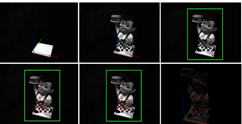
Figure 3.1: The database of features for the object is generated during a training phase. Beginning with the top row, far left, the training phase begins by establishing a set of coordinate axes for the object using a calibration platform. Once established, the object axes is aligned with the axes of the platform (top row, middle image). A bounding box is then dened by the user around the object in the image (top row, far right), where feature extraction is to be applied (bottom row, far left). Features within the bounding box though not part of the image are then removed as shown in the bottom row, middle image (note the features on the white platform have been removed). In the nal step, full stereo is applied and nearest-neighbor data association is applied to assign each extracted feature a corresponding 3D point, as dened in the object-reference-frame.
evaluated at the predicted pose location:
Ck =
∂H
∂Xk X
k .
The full analytical expression forCk can be found in Appendix A. The matrix Kk is the dynamic Kalman gain as dened in equation (2.9) and reproduced here for reference:
Kk=PkCTk(Ck·Pk·CTk + Σm)−1 .
With the dynamic prediction step and measurement update step of Bayes' Filter dened, the recur-sive algorithm can be implemented in a sequential fashion as discussed in section 2.1.2. However, it is important to note that the measurement update is contingent upon accurate specication of the feature correspondence variable,J, which is discussed in section 3.2.4.
3.2.3 Training Phase
3. When the object is stabilized and properly aligned with the anchored coordinate axes, the live image from the reference camera is displayed and a user dened bounding box is drawn around the object (Fig. 3.1, top row, right).
4. Feature extraction is then applied to the region of interest dened by the bounding box (Fig. 3.1, bottom row, left).
5. Once the set of features in the region of interest are generated, features not necessarily belong-ing to the object (though still within the boundbelong-ing box) are removed manually in a touch-up step (Fig. 3.1, bottom row, middle).
6. Once extraneous extracted features are removed, the remaining features are assigned nearest neighbor 3D stereo data points, where nearest-neighbor is determined via Euclidean distance in pixel coordinates between the feature location and the projected stereo location in the image plane. However, before tagging features with their corresponding 3D stereo location, the 3D stereo data points are transformed into the object reference frame using the coordinate axes dened in step 1 (Fig. 3.1, bottom row, right).
7. Steps 16 are then repeated for each additional viewpoint.
Following the training phase, the set of database features is stored to a series of data les indexed by viewpoint and object ID. Thus the above steps need only be executed once for each object since any subsequent queries for detection and tracking for that object can be done by loading the appropriate set of data les.
3.2.4 Feature Matching
frequency of false alarms and mismatches, and computational cost the best overall choice reduced to features with SIFT descriptors but detected using an ane-rectied detector (as dened by Mikolajczyk and Schmid in [33]) instead of the Dierence of Gaussians detector proposed by Lowe in [30]. However, the authors acknowledge that for increased computational speed, the Dierence of Gaussians detector can be used since its performance is comparable to the ane-rectied detector. As such, the approach presented here considers SIFT features detected using the Dierence of Gaussians detector.
With regards to nding a method of searching through potentially thousands of features to nd the correspondences, exhaustive search is guaranteed to be optimal. However, its computational expense has promoted other approaches. A popular method and the one adopted in this framework is the Best-Bin-First search method rst presented by Beis and Lowe in [2]. In their search method, the authors dene an approach that uses a k-d tree to bin up the feature space so that features are searched in order of distance from the query location. Note that their approach is not an exhaustive search since the tree search is cut o after a certain number of bins have been explored. Additionally, valid matches are only considered if the ratio of the current best match to the second best match is less than a threshold (in their case, 0.80). While their approach does not necessarily always return the true correspondence, it will at least return the true feature correspondence with high probability. Given that inaccurate feature correspondences can lead to erroneous pose estimates, a remedy commonly implemented by others is to add an additional coherency check to validate correspon-dences ([54], [40], [5]). In the approach presented, a geometric model check is similarly employed. Supposing an object is already being tracked, then for each correspondence found from SIFT feature matching, the matched 3D database feature is transformed into the camera-reference frame and the Mahalanobis distance between the transformed feature and its matched current feature (in Euclidean space) is checked against a threshold. If the distance exceeds the threshold, the correspondence is rejected. If an object is not yet initialized, the geometric constraint is not applied, since the object
5It is important to note the authors' distinction between a detector and a descriptor. A detector is any interest
algorithm or pose re-initialization after a lost track. Once a track is established, SIFT is essentially turned o and sustained tracking is realized by faster, computationally less-expensive algorithms (i.e., POSIT, Lucas-Kanade Tracker, Contracting Curve Density (CCD) algorithm, etc.). To get a perspective on the delays associated with SIFT feature extraction (without sparse stereo), a typical 320×240 image will take on average 200 ms to compute 70+ features in an image on a 2.40 GHz
processor (and >200 ms for high context images that can contain several hundred SIFT features); that means at most, a 5 Hz performance rate can be achieved assuming the remaining computations associated with sparse stereo, feature matching, and the steps of Bayes' Filter are negligible in computational costs.
In the approach presented here, SIFT feature extraction is used for track initialization and also for sustained tracking. Real-time calculations with SIFT are achieved by noting that much of the expensive operations involved with feature extraction are spent on areas of the image not containing the object. Assuming the object pose is known, a region of interest (ROI) can be specied that bounds a subset of the image known to contain the object. By specifying a ROI in the image, SIFT feature extraction can be reduced to operating in a window size typically 10%-40% of the original image, thus making real-time pose tracking with SIFT possible. Of course the ROI cannot be specied if the object pose is it not known and SIFT must be applied to the entire image reducing the proposed approach to an initialization step no dierent than the approaches of Choi et al. [5] and Panin and Knoll [40].
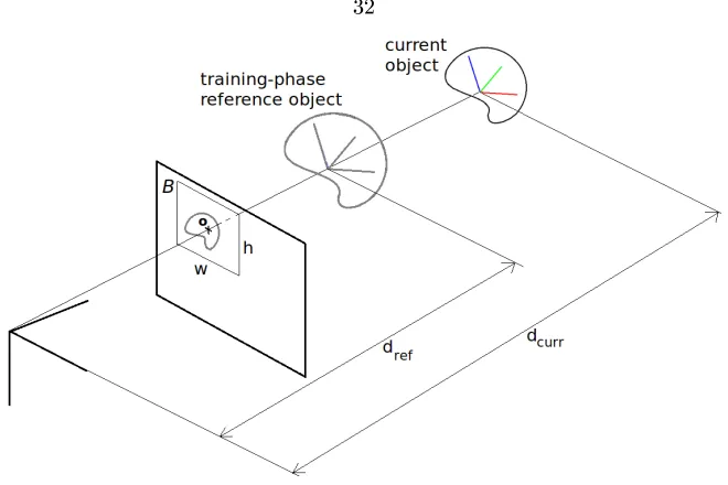
Assuming an object track has been initialized, the ROI is determined as follows: leto∈R2×1be
the projected object origin onto the image plane of the reference camera, B = [x y w h]represent
a bounding box dening the ROI of the image (x and y the center of the ROI, and w and hthe
width and height), dref ∈ R be the reference distance dened as the nominal Euclidean distance
between the camera and the object reference frames during training as described in section 3.2.3, anddcurr∈Rbe the current distance between the camera origin and the object origin (Figure 3.2
Figure 3.2: The ROI of the current image is centered on the object origin (projected into the image plane), with width and height computed based on the scaled ratio of the reference object distance to the current object distance.
to be determined. xandy will come from the projection of the object origin onto the image plane:
x=f·X
Z +cx, y=f·Y
Z +cy,
where (X, Y, Z) represent the current 3D location of the object origin in the camera-reference
frame,f the focal length of the camera, and (cx,cy) the image center of the reference image. As for
the widthwand heighth, these parameters of the ROI are dened as follows:
w=kx·σs,
h=ky·σs,
wherekxandky are constants (dependent on the size of the object) and σs a scaling factor dened as
σs=
dref
dcurr
.
Figure 3.3: The overall approach for the presented algorithm is summarized in the above gure which describes the series of steps taken from input to output for one iteration.
3.3 Approach Summary
To summarize the overall approach, Fig. 3.3 outlines the basic steps for one iteration of the algo-rithm. It begins with the input, which is the pair of stereo camera images. SIFT feature extraction is then applied to the reference image of the stereo pair using the Region of Interest (ROI) if the object track has already been initialized. This step also incorporates 3D coordinates being assigned to each extracted feature using sparse stereo calculations. Following SIFT feature extraction, fea-ture matching is then applied using the Best-Bin-First algorithm of Beis and Lowe [2]. Geometric constraint checks are then applied depending on whether the object track has been initialized. The purpose of this step is to remove geometrically infeasible correspondences that may have resulted from the matching step. The nal step of the algorithm is to apply the recursive Bayes' Filter equations (EKF), which yields a pose estimate of all 6 Euler parameters for thekth timestep.
3.4 Experimental Results
Based on the analysis presented thus far, two types of experiments were considered to validate the real-time capabilities of the 3D pose tracking algorithm. An object in this case a Bob's Big Boy model bank was trained using the training phase discussed in section 3.2.3 and used as the test object in both experiments. Eight viewpoints were considered during training, with each viewpoint positioned at 45◦ intervals about the object spanning a full 360◦ along the equidistant
ring yielding a total of 1482 features stored in the database. For a stereo camera, a PointGrey Research BumbleBee2 stereo color camera with a native resolution of 640×480 downsampled to
320×240 was used for both experiments. The computing platform used was a laptop running
Figure 3.4: The image on the left shows the setup for the rst experiment considered (uncluttered en-vironment). The image on the right shows the setup for the second experiment considered (cluttered environment with noise).
optimized speed. The open source Intel library, OpenCV,6 and the 3D rendering library, OpenGL,7 were also used to develop the system. Fig. 3.8 shows a screenshot of the visual interface used in the experiments.
In the rst experiment, the trained object was positioned in an uncluttered environment (uniform background with no other objects) and placed under continuous rotations and translations in all degrees of freedom with the camera stationary and measurements made in the camera reference frame. The purpose of this experiment was to test the baseline capabilities of the presented approach in tracking all six Euler parameters. In the second experiment, the trained object was placed in a cluttered environment (noisy background with other similarly sized objects) and again placed under continuous rotations and translations with the camera stationary. The purpose of this experiment was to test the capabilities of the approach to robustly track 3D pose estimates against non-uniform noisy backgrounds and partial occlusions. Fig. 3.4 shows the setup for both experiments.
In both experiments, a measure of ground truth was essential in comparing the accuracy of the estimated results. The next section describes an approach to acquire ground truth estimates of all six Euler parameters. In comparison to prior work, this method does not require the purchase of third party software as in [54], simulated experimental results as in [40], or distinguishing markers for computer vision toolkits as in [5] which in itself is just another form of a position estimate with noisy data.
3.4.1 Ground Truth
Ground truth for both experiments was determined by using a controllable stepper motor in this case, a Directed PerceptionT M,8PTU-D46-17 pan-tilt-unit with an accuracy of0.0514◦ in both pan
and tilt positions (though tilt positioning was not used). The base of the motor (reference frameB)
6http://opencv.willowgarage.com/wiki/ 7http://www.opengl.org
Figure 3.5: The various frame transformations between camera (C), platform (P), and object (O) can be measured to establish a means of object ground truth, as measured in the camera reference frame.
was rigidly mounted to a table and a platform was xed to the pan axis of the motor (reference frame
P), rigid enough to support the weight of the object being detected. The object (reference frame O) was then placed on the platform, a xed distance from the pan-axis, though with the object's
vertical axis aligned in the same direction. The stereo camera (reference frameC) was then placed
some xed distance away from the motor base-frame, pitched looking slightly downwards, and kept stationary (see Fig. 3.5 for a clear depiction of all various reference frames). Commanded rotations resulted in rotations and translations of the object as seen in the camera reference frame.
With this particular setup, all 6 Euler parameters would be known to high accuracy since the transformations between all frames could be easily measured. Because the camera was kept station-ary in both experiments, the transformation between the base of the motor frame and the camera frame was a constant, measurable value:
GCB =
RCB dCB
0T 1
∈SE(3) .
For each pan rotation commanded to the stepper motor, the transformation between the platform frame and the base frame could be determined by the motor angle read out (φk):
GBP =
RBP(φk) 0
0T 1
∈SE(3) .
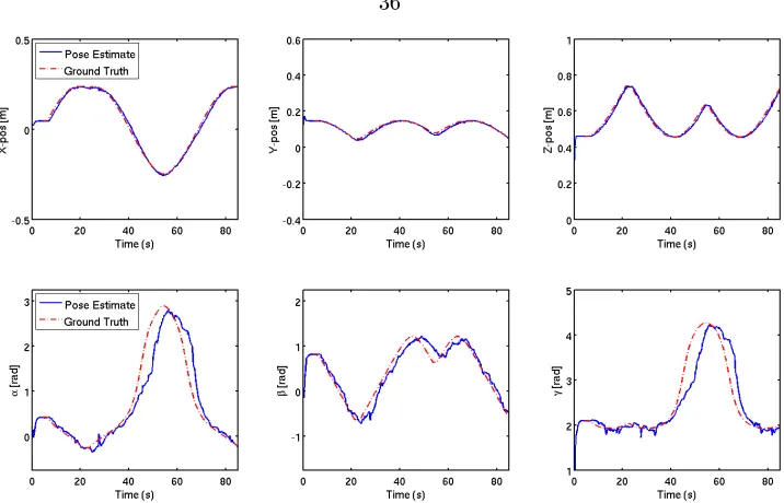
Figure 3.6: Shown above are the 6 Euler parameter estimates using the algorithm described for the rst trial experiment where the trained object was placed in an uncluttered, uniform environment. The top row shows the tracking results in (x,y,z) and the bottom row shows the results in (α,β,γ).
Shown in the red dotted line is the ground truth measurements of the Euler parameters, and in blue the EKF-estimated Euler parameters.
(needed only inxandy) and the rotation (needed only about thez-axis) between frames:
GP O=
RP O dP O
0T 1
∈SE(3) .
Finally, by measuring the transformations GCB, GBP, andGP O, the ground truth transformation between the object and camera can easily be determined as
GCO,truth=GCB·GBP ·GP O.
3.4.2 Uncluttered Environment
As mentioned earlier, in this experiment the trained object was positioned in an uncluttered environ-ment having a uniform background with no other distractors present. The trained object was placed under continuous rotations and translations in a manner as described in section 3.4.1. The platform itself oscillated between+90◦ and−90◦ at a slew rate of6◦/s. The purpose of this experiment was
to test the baseline capabilities of the presented approach in tracking all six Euler parameters. Shown in Fig. 3.6 are the results for this experiment. As can be seen in the gure, in this most basic scenario the algorithm does an extremely good job of tracking the object in (x,y,z). With
regards to orientation, the estimated values of (α,β,γ) are slightly noisier and subject to minor
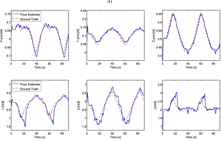
Figure 3.7: Shown above are the 6 Euler parameter estimates using the algorithm described for the second trial experiment where the trained object was placed in a cluttered, noisy environment. The top row shows the tracking results in (x,y,z) and the bottom row shows the results in (α,β,γ).
Shown in the red dotted line is the ground truth measurements of the Euler parameters, and in blue the EKF-estimated Euler parameters.
platform rotates, which when matched, causes the EKF to improve the overall estimate and reduce the state covariance.
With regards to real-time tracking capabilities, the algorithm ran at an average rate of 12.12 Hz, with a maximum rate reaching 21.40 Hz. Because of the manner in which the ROI is computed, the algorithm actually performs faster as the object moves away from the camera (smaller ROI) reaching a nominal 20 Hz frequency rate, and slows down to about 8 Hz when the object comes closer (larger ROI).
3.4.3 Cluttered Environment
In this second experiment, the trained object was placed in a cluttered environment (noisy back-ground with other similarly sized objects) and again placed under continuous rotations and trans-lations with the camera stationary. As stated earlier, the purpose of this experiment was to test the capabilities of the presented approach to robustly track 3D pose estimates against non-uniform noisy backgrounds and partial occlusions. Using the same trained object, the platform was rotated this time between+60◦ and−60◦ at a slew rate of 6◦/s to generate the necessary translations and
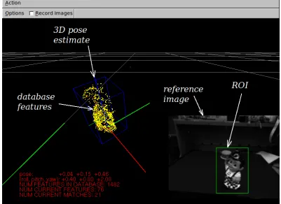
Figure 3.8: A screenshot of the algorithm running in real-time. For clarity, aspects of the developed visual interface have been annotated to illustrate the details of the algorithm working.
occlusions.
Shown in Fig. 3.7 are the results for this experiment. As can be seen in the gure, the tracking results in (x,y,z) and in (α,β,γ) are denitely noisier than in the rst trial experiment, which is
expected given the noisier image scene and partial occlusions. There is also a similar delay in the orientation estimates which is prominent at the peaks of the oscillating platform. Similar to the rst experiment, this eect is most likely due to certain features coming into view as the platform rotates, which when matched, causes the EKF to improve the overall estimate and reduce the state covariance. It is more prominent in this experiment mainly due to the occlusions caused by the other objects surrounding the object being detected.
Identication
Building on the framework for pose estimation presented in chapter 3, the additional problem of sensor planning for object/model identication is considered. This chapter addresses the combined problem of sensor planning for object identication with 3D pose estimation by contributing a novel algorithm derived from basic Bayesian principles. Optimal control actions for sensor placement are achieved via an information gain metric based on current and future measurements conditioned on estimated 3D object poses for all possible models. The following sections present the proposed algorithm in full detail. Experimental validation of the algorithm is presented in chapter 5, which will illustrate the success of the approach and the novelty of the contribution. This chapter will focus on the derivation and details of the algorithm.
4.1 Sensor Planning Context and Contribution
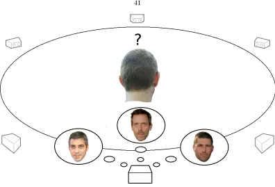
Figure 4.1: An illustration motivating the problem addressed in this chapter. A robot is tasked with identifying an unknown object (in this case a person) from a set of known objects. If the object identity is indistinguishable from a nite set of similar models, the robot must then decide where to move next to best acquire the most relevant information that helps resolve the identity of the unknown object.
4.2 Bayesian Sequential Analysis and Formulation
Consider the case of an autonomous robot which is given a database of known models for objects that may exist in its environment. Now suppose an unidentied object, though belonging to the database of known objects, is presented to the robot which is now tasked with identifying the correct object model and estimating its 3D pose. The question then arises: if the robot is unable to identify the correct model in the initial presented view, how should it optimally move to identify the object?
4.2.1 Approach
LetDkdenote visual (and possibly other) data obtained attk (e.g., this data might consist of SIFT features [30], Harris corners, 3D range points, etc.) and letuk be the control input attk.1LetXk,i be the system state vector attk for the ith model,Mi (this state could be the state of the object relative to the camera, or the state of the camera relative to the object, etc.). For a given modelMi,
state Xk,i, and measurement data Dk, suppose its evolution in time is governed by the following
1The notation1 :kwill be used to indicate the set of measurements, inputs, etc. fromt
Iuk =H(M|D1:k,u1:k−1)−EDk+1[H(M|D1:k+1,u1:k)]. (4.3)
The term,H(M|D1:k,u1:k−1), is the conditional entropy of the model identity, conditioned on the
data up untiltk and the control actions up untiltk−1. The term,EDk+1[H(M|D1:k+1,u1:k)], is the
expected conditional entropy, with the expectation taken over the future data at the next timestep, i.e., Dk+1, after hypothetical controluk is applied. Note that with this denition of the expected conditional entropy, a myopic approach to sensor planning is assumed (i.e., a one step lookahead).
Entropy is understood to represent the uncertainty associated with a random variable, which in this case is the model identity, M. Thus the larger the entropy, the greater the uncertainty
associated with the model being identied. It make sense, then, that the optimal control action is the one which maximizes the expected information gain:
u∗=argmax uk
Iuk , (4.4)
since information gain occurs when H(M|D1:k,u1:k−1)> EDk+1[H(M|D1:k+1,u1:k)], or when the
next applied control results in an expected reduction in the uncertainty of the model identity. Considering the information gain as dened above, the remainder of this section expands the expression for Iuk. It will be seen that the state of the system (the object 6D pose) becomes a
necessary estimation step in determining the optimal sensing action. The core entropy terms can be expanded as follows:
<